Sage Journals: Discover world-class research

Abstract

Objectives

Morphologic information from bone marrow (BM) examinations remains critical for diagnosing leukemia and lymphoma, yet manual interpretation of BM smear slides is labor-intensive for hematologists and pathologists. Few automatic diagnostic tools have successfully classified whole slide images (WSIs) of hematologic malignancies. This study aimed to develop a deep convolutional neural network (DCNN) pipeline to classify leukemia subtypes and lymphoma using whole-slide BM aspirate images.

Methods

The process involved two stages: first, a quality assessment model selected 200 regions of interest (ROIs) from each WSI to exclude non-informative areas. Next, eight DCNN models with different architectures were trained to classify each ROI into one of five hematologic malignancies, and tile-level predictions were aggregated to produce patient-level results. External evaluation and ancillary analyses were performed to demonstrate generalizability and robustness.

Results

In total, 1,022 WSIs were enrolled. The results showed average patient-level accuracy, balanced accuracy, F1-score, and area under the receiver operating characteristic curve (AUC) of 95.2%, 94.7%, 94.8%, and 0.993, respectively, with DenseNet121 achieving the highest balanced accuracy (97.6%). Our method outperformed clustering-constrained attention multiple instance learning (CLAM) in comparison study (accuracy 97.1% vs. 85.0%) and reached accuracies of 83.8% and 86.7% on external datasets. Visualization maps showed consistency between model salience and cell distribution.

Conclusion

Our results demonstrate the ability of DCNNs to achieve accurate diagnosis in hematologic pathology, and the pipeline holds potential to assist in early diagnosis and workflow augmentation for hematologists and pathologists.

Keywords

hematologic malignancy whole slide image multiple instance learning deep convolutional neural network

Introduction

Hematologic malignancies, a substantial component of the global oncologic burden, account for approximately 1.3 million new cases and 730,000 fatalities annually worldwide. The incidence of these neoplasms has steadily increased over the past three decades.¹ In 2025, the United States is expected to report 192,070 new cases and 56,110 deaths from hematologic malignancies.² Obtaining an accurate and timely diagnosis is essential to treatment planning as well as prognosis prediction in hematologic neoplasms. Both the 5th edition of the World Health Organization Classification of Hematolymphoid Tumors (WHO-HAEM5) and the International Consensus Classification (ICC) have relied more heavily on molecular and genomic studies,³ whose turnaround time, however, can last from three days to even weeks.⁴ Bone marrow aspirate smears, which can be prepared within six hours,⁵ provide immediate information regarding morphology, linage assessment, and differential count, possessing high diagnostic value before the report of molecular testing results.⁶ The latest WHO-HAEM5 still preserves essential diagnoses that are diagnosed via traditional morphology,⁷ and ICC also includes myeloblast percentage in the criteria of AML classification.⁸ However, the interpretation of bone marrow aspirate slides is prone to inter-observer variability, drudging for pathology departments in medical centers, and difficult for institutions with a lack of experienced hematopathologists.⁹ An automated diagnostic tool that can classify multiple hematologic malignancies from BM slides can, therefore, accelerate diagnosis at initial encounters across all levels of healthcare providers.

Owing to remarkable progress in computational power and data storage, machine learning (ML)–based models have been extensively investigated and proven successful in visual assessment across multiple medical disciplines.¹⁰ As a subset of ML, deep learning (DL) has become the mainstay by yielding models with even more satisfactory performances, including the deep convolutional neural network (DCNN).^11,12 In hematology, high performances have been attained not only in single disease classification including acute lymphoblastic leukemia (ALL),^13,14 acute myeloblastic leukemia (AML),^15–17 and lymphoma,¹⁸ but also in multiple disease classification.^19–22 Promising though these studies were, all their DCNN required manual localization or selection of regions of interest (ROIs), which limited the development of a fully automated classification pipeline.

Whole slide images (WSIs), referring to digitized images of the entire glass slide at a resolution sufficient enough to render a diagnosis, have proven valid as an alternative to light microscopy when diagnosing lymphoma.²³ Since the direct application of DCNN on WSIs is so far infeasible due to the extremely large number of pixels, researchers have devised multiple automated strategies to select relevant ROIs or to refine feature vectors extracted from multiple ROIs. Kockwelp et al.²⁴ filtered out cell patches with poor quality, reaching near 83% accuracy in the identification of NPM1 and FLT3 mutation status of AML. Wang et al.²⁵ ameliorated the clustering-constrained attention multiple instance learning (CLAM) framework, calculating a weighted average of all feature vectors without a need for ROI selection. They accomplished 90% accuracy in classifying AML, ALL, chronic myelocytic leukemia (CML), chronic lymphocytic leukemia (CLL), and multiple myeloma (MM) WSIs, which marked the first study to perform multiple hematologic disease classification automatically on WSIs.

In this study, we sought to implement a two-stage pipeline to classify WSIs of bone marrow aspirates into ALL, AML, CML, lymphoma, and MM, as shown in Figure 1. An automated ROI selection process using DCNN marks the first stage of our approach, and in the second stage, another DCNN predicts the disease label according to the selected ROIs. We evaluated the results on a separate test set as well as external datasets, and conducted subgroup analysis, comparison study, and ablation study as ancillary evaluation for robustness and generalizability. We aim to prove the feasibility of DL neural networks to classify hematologic malignancies on WSIs through ROI tile selection and instance aggregation, and to assist clinicians with initial disease management.

Figure 1.

Graphical abstract of our two-stage automatic whole slide image (WSI) classification model. After a bone marrow (BM) aspirate smear was stained and scanned, the WSI was cropped into tiles with 256 pixel wide overlap. The quality assessment model selected only 200 tiles with high quality scores as regions of interest (ROIs). Next, eight disease classifiers were trained to yield tile-level predictions for each selected ROI. To implement multiple instance learning, 200 predictions were aggregated with a majority voting method to yield a patient-level prediction, and patient-level predictions from eight classification models were aggregated again to obtain an ensemble-level prediction. Lastly, visual explanations with saliency maps were produced on the tile level as well as WSI level (not shown) to provide intuitive hints for clinicians and hematopathologists. P_{n, c} indicates probability of the n^th tile being class c. CAM, class activation map.

Methods

Patient recruitment and slide preparation

We collected bone marrow aspirate specimens obtained at the time of diagnosis from treatment-naïve patients with hematologic malignancies at Taipei Veterans General Hospital, Taiwan, between November 2005 and April 2023. Clinical diagnoses included ALL, AML, CML, MM, and lymphomas (including CLL), all of which were established by experienced hematologists in accordance with the WHO Classification of Tumors of Hematopoietic and Lymphoid Tissues.²⁶ Cases with normal cytology and morphology were excluded from the cohort, as such findings typically indicate heterogeneous or complex etiologies.^27,28 The study was approved by the Taipei Veterans General Hospital institutional review board (no. 2023-10-010AC).

All bone marrow specimens were aspirated from the iliac crest. The cytologic smear slides of bone marrow aspirates were stained using the Wright-Giemsa method (Supplemental Table 1) and were scanned into WSIs with a Pannoramic SCAN scanner (3DHistech) with 40× magnification. In some WSIs, rectangular regions where auto-focus failed were manually removed. We tiled each WSI into images of size 512 × 512 pixels using the OpenSlide Python library.²⁹ To prevent information loss of cropped cells at tile borders, adjacent tiles were taken by an increment of 256 pixels in either X or Y direction. As plain white or plain black pixels likely represent background or artifacts, we excluded tiles whose corner pixels contained these two colors in advance.

Stage 1: Tile selection based on quality

In this step, we trained a DCNN model based on the VGG-16 architecture to predict the probability that a single tile is of good quality. Using a human-in-the-loop approach modified from Eckardt’s study,¹⁷ we repeatedly sampled thousands of validation tiles from new slides, evaluated the model with validation tiles, corrected the model’s prediction, and fine-tuned the model with both validation tiles and previous tiles. The loop ended when fewer than 5% of validation predictions were incorrect. The above verification was conducted by an experienced hematologist (C.-J. L.), and a tile was labeled poor quality if any of the following conditions existed: (a) containing fewer than ten nucleated cells, (b) containing overlapping nuclei, (c) containing obvious adipocyte or artifact, or (d) all cells were located in the peripheral areas.

To obtain tiles with good quality from a single WSI, all tiled images from the same slide were evaluated using the model trained above. We then randomly selected 200 ROI tiles with output probabilities ≥ 0.8 to represent the WSI during the second stage disease classification. If fewer than 200 tiles could be recruited with threshold 0.8, a lower threshold of 0.5 was determined, and WSIs with fewer than 200 tiles that had probabilities greater than 0.5 were excluded from the cohort. To verify the effectiveness of quality-based ROI selection, we also conducted an ablation study where stage 1 was replaced with random sampling of 200 images from all non-background tiles. Representing the WSIs, these random tiles underwent subsequent test-train split, training, and aggregation same as the selected ROIs, and we compared the classification results on the test set eventually.

Stage 2: Disease classification based on selected tiles

Dataset preparation

The included WSIs were split into training, validation, and test sets for the second stage in the proportion 6:2:2. Such a per-subject splitting method avoids overestimation of performance due to “data leakage”³⁰ by ensuring that all tiles from the same patient exist in the same set. ROI tiles were assigned with ground truth labels equal to the diseases of the WSIs they belonged to. During model training, each tile image underwent random flipping, rotation between 0 and 360 degrees, and zooming between 90% and 110% before being sent as input, a process known as “augmentation”.³¹

Transfer learning and CNN architectures

To establish second-stage models, we obtained eight open-source base models as backbones to build up our classifiers. These public models, using CNN architectures including VGG-16,³² Inception-V3,³³ ResNet50,³⁴ DenseNet121,³⁵ MobileNetV3Large,³⁶ NasNetMobile,³⁷ ConvNeXt-Tiny,³⁸ EfficientNetV2B3,³⁹ were well-trained to classify natural images on the ImageNet database. For each model, we replaced the original classifier layers with a newly initialized classifier, which possessed five normalized outputs predicting probabilities of a tile being ALL, AML, CML, lymphoma, or MM.

As the prevalence of different diseases differs, class imbalance has been a common issue in machine learning and can produce a prediction bias toward major classes, thereby increasing false negative rates of minor classes.⁴⁰ To address this, class weights were applied. The categorical cross-entropy loss of a specific class C was multiplied by a penalty W_C that was grossly inverse-proportional to the sample size of C:

W_{C} = \frac{N_{P}}{N_{C} \times N_{c l a s s e s}}

(1)

where N_P denoted the sample size of the entire training set, N_C denoted the sample size of class C, and N_clases denoted the number of classes. By increasing the loss of minor classes, the neural network, theoretically, adjusts its weights more avidly for minor classes.

Transfer learning was applied at this stage to reduce computational burden and training time. Firstly, a larger learning rate (0.005) was applied to adjust the parameters of the new classifier layers only. Secondly, a smaller learning rate (0.0005) was applied to train both the classifier and the base model for 35 epochs, a process known as “fine-tuning”. The model was evaluated on the validation set after each epoch, and the one with the best validation accuracy was saved. A stochastic gradient descent (SGD) optimizer was used across all training processes The neural networks were built upon the Tensorflow platform (version 2.11), run with Python 3.9.16, and trained on Harvard Medical School’s Orchestra 2 Cluster.

Inference on test set

During the testing stage, the tiled test set images were totally unseen, and three levels of class predictions were inferenced without augmentation. Firstly, the saved models were evaluated directly on the tile level by pooling all ROIs together. Secondly, for each WSI, we applied majority voting to acquire a patient-level prediction, which was the disease with most occurrences within the 200 tile-level predictions. A Wilcoxon signed rank test was applied to examine whether patient-level accuracies of eight final models were significantly different from tile-level accuracies. Thirdly, an homogeneous ensemble-level prediction⁴¹ was acquired by aggregating tile level predictions across eight saved models for a single WSI.

Performance evaluation statistics

Several statistical methods have been devised to evaluate the performance of multiclass classifiers.⁴² The confusion matrix summarizes the frequencies of all possible ground truth–prediction pairs in an $N_{C l a s s e s} \times N_{C l a s s e s}$ table, as illustrated in Figure 2. This matrix simultaneously conveys the class distribution of the dataset and the classification tendencies of the model. In the following context, $i$ denotes the ground truth label, $j$ the predicted label, and $n_{i, j}$ the frequency of the $(i, j)$ label combination. The diagonal elements, denoted $n_{i, i}$ , represent correct predictions in which the predicted labels match the corresponding ground truth labels. To account for class imbalance, the unnormalized values $n_{i, j}$ can be divided by the total number of samples in class $i$ , yielding a normalized confusion matrix in which each element is expressed as $n_{i, j} / \sum_{j} n_{i, j}$ . In this normalized representation, the diagonal elements ( $n_{i, i} / \sum_{j} n_{i, j}$ ) correspond to the sensitivities of the respective disease classes.

Figure 2.

Patient-level confusion matrices and ROC curves of the selected DenseNet121-based model. (a) Unnormalized confusion matrix showing original numbers of patients of each ground truth-prediction combination, where darker color indicates a larger number. (b) Normalized confusion matrix in which each entry is divided by the number of patients of that ground truth class; the diagonal entries are also sensitivities of their corresponding disease classes. (c) ROC curves plotted using the one-vs.-rest method. AUCs are shown in the figure legend, and the dotted diagonal line indicates the curve of a random model. (d) ROC curves plotted using the micro-average and macro-average methods, showing AUCs of 0.992 and 0.997, respectively. (e) Micro-average ROC curve with 95% CI calculated with bootstrap algorithm, showing an AUC 95% CI of (0.987–0.997). ALL, acute lymphoblastic leukemia; AML, acute myeloblastic leukemia; CML, chronic myelocytic leukemia; MM, multiple myeloma; ROC curve, receiver operating characteristic curve; AUC, area under curve; CI, confidence interval.

Next, we applied the following metrics in our study, all of which can be derived from confusion matrices.

A c c u r a c y = \frac{\sum_{i} n_{i, i}}{\sum_{i} \sum_{j} n_{i, j}}

(2)

B a l a n c e d A c c u r a c y = \frac{\sum_{i = 0}^{4} {R e c a l l}_{i}}{5} = \frac{\sum_{i = 0}^{4} (\frac{n_{i, i}}{\sum_{j = 0}^{4} n_{i, j}})}{5}

(3)

F 1 ‐ s c o r e = 2 (\frac{M a c r o a v e r a g e r e c a l l \times M a c r o a v e r a g e p r e c i s i o n}{M a c r o a v e r a g e r e c a l l + M a c r o a v e r a g e p r e c i s i o n})

(4)

While accuracy creates a bias towards classes with higher frequencies, balanced accuracy and F1-score do not shield a model’s performance on smaller classes by assigning equal weights to all disease categories.⁴³

The receiver operating characteristic (ROC) curve along with the area under the curve (AUC) provides the overall summary of diagnostic accuracy of a model in binary classification tasks.⁴⁴ We applied the micro-average method to dichotomize our five-class classification problem, which assigned larger weights to major classes. AUCs of all ROC curves were calculated, and we reported 95% confidence intervals (CIs) using the bootstrap method.

Ancillary analyses

Comparison study

We adopted a clustering-constrained attention multiple instance learning (CLAM) neural network model to objectively assess our pipeline. The process begins by extracting low-dimensional feature embeddings from all tiled patches. CLAM then utilizes a gated attention network to calculate an attention score for each instance, allowing the model to “attend” to the most diagnostically relevant regions by assigning them higher numerical weights during the aggregation phase. Also, the “clustering-constrained” aspect of the framework introduces a supervised learning task to ensure that the learned features are representative of the specific disease classes, thereby enhancing the discriminative power of the model even in the absence of explicit ROI selection. This framework has demonstrated high diagnostic performance, achieving AUC values exceeding 0.95 across multiple disciplines, including lung cancer, renal cell carcinoma, and lymph node metastasis.⁴⁵

The CLAM model in our study was based on ResNet-50 feature extractor, and trained, validated, and tested with split patient cohorts identical to what we built our pipeline with. An early-stopping strategy according to validation loss was also adopted to prevent overfitting. As CLAM models produce slide-level outputs without instance-level ones, we compare the results only at the patient level.

Ablation study

In our pipeline, each WSI was processed through a quality-based ROI selection stage and a classification-aggregation stage to obtain a patient-level diagnosis. We examined the effectiveness of the first stage by replacing the model-selected ROIs with randomly-selected ones. Subsequently, with identical test-train split and training settings, we trained another DenseNet121 classification model using these random tiles and evaluated its patient-level performance on the test set.

In comparison, to evaluate the effectiveness of the second classification-aggregation stage, we kept only the tile classification step and omitted patient-level aggregation. The methodology was identical to evaluation on the tile level, which we reported in the main result.

Subgroup analysis

To test the generalizability of our method, we performed subgroup analysis to examine the performance on patients with different tumor burdens. We calculated blast cell percentage and neoplastic plasma cell percentage of AML and MM WSIs respectively given their larger sample size. Within each disease, cases were dichotomized into high- and low-blast-percentage groups using the disease-specific 50th percentile of cell percentage as the cutoff. We then reevaluated model performance within each subgroup using the same patient-level aggregation strategy described above and reported the accuracy and micro-averaged AUC.

External validation

Next, we obtained two external datasets to evaluate the generalizability of the best-performing model among eight architectures. The first outer cohort consisted of 74 whole slide bone marrow aspirates of patients with ALL, AML, and MM from Kaoshung Veterans General Hospital, which were stained with Wright-Giemsa method and captured under 40× magnification. The WSIs were tiled and preprocessed in the same way as our test set and evaluated at both the tile and the patient level.

The second was the public SN-AM dataset, which was made up of 30 B-cell ALL and 30 MM images taken from bone marrow aspirates under 1000× magnification. Originally designed to test stain normalization methodology, the images were highly variable in color spaces,⁴⁶ and we applied the Reinhard algorithm⁴⁷ for stain normalization. Also, to maintain height-to-width ratio and magnification, the center 1728×1728 pixels were cropped as the ROI for each image. As SN-AM dataset includes only one image for each patient, we evaluated the tile-level performance merely.

Visual explanation of selected models

We adopted the gradient class activation map (grad-CAM) proposed by Selvaraju et al. in our study to generate colormaps, which accentuated regions in a ROI that contributed most to a model’s prediction. Given a CNN layer and an output class of interest, grad-CAM was defined as the weighted average of all feature maps within the selected CNN layer, where the weights equaled the pooled partial derivatives of the selected output probability with respect to the corresponding feature maps.⁴⁸

To acquire a WSI-level interpretation, we collected the coordinates of all tiled images that were selected to enter the classification stage and created a scatter plot by superimposing these coordinates on their corresponding WSI thumbnail image. Furthermore, we generated an ROI density map as well as a prediction probability map with spatial interpolation, and took the Hadamard product of these two matrices as the saliency map. Superimposing the map on the WSI, this visualization provides a hint of informative regions for pathologists if manual review is required in certain clinical settings.

Results

Dataset preparation and patient characteristics

We retrospectively identified 1,119 scanned BM aspirate slides, including 115 ALL, 382 AML, 75 CML, 318 lymphoma, and 229 MM WSIs. Among the 382 AML patients, 36 were diagnosed with APL, while 86 of the 318 lymphoma patients were compatible with CLL/SLL. After multiple loops of training and expert verification, a first-stage model was established to identify tiled images with poor quality. We then applied the model to all automatically cropped tiles of the WSI cohort, where 97 slides were excluded for having fewer than 200 qualified tiles. In this stage, only 10,789 tiles were manually reviewed, which is less than 0.05% of the number of tiles in the entire dataset.

In a disease-stratified randomized manner, we divided the remaining 1,022 slides into training, validation, and test groups in a proportion of 6:2:2, and the number of patients in each group is shown in Supplemental Table 2. A total of over 24 million (24,871,994) tiled images was collected from all WSIs, with a single WSI yielding 24,336 tiles on average (Supplemental Table 2). The median ages of ALL, AML, CML, lymphoma, and MM cohorts were 37.5, 62.0, 61.0, 66.0, and 70.0, respectively. While patients with ALL had the youngest age of onset, patients with MM had the lowest CKD-EPI estimated glomerular filtration rate. Other detailed baseline characteristics are provided in Table 1.

Table 1.

Patient characteristics of the total study cohort.

Characteristics	ALL	AML	CML	Lymphoma	MM
Characteristics	n = 100	n = 338	n = 82	n = 289	n = 213
Age, median (IQR) —	37.5 (38.0)	62.0 (25.8)	61.0 (28.5)	66.0 (18.0)	70.0 (21.0)
Male sex, n (%)	57 (57.0)	187 (55.3)	45 (54.9)	173 (59.9)	119 (55.9)
Comorbidities
Diabetes mellitus, n (%)	33 (33.0)	102 (30.2)	49 (59.8)	144 (49.8)	57 (26.8)
Hypertension, n (%)	37 (37.0)	100 (29.6)	52 (63.4)	156 (54.0)	55 (25.8)
Laboratory data
WBC, median (IQR) —/μL	15,905.0 (51,007.5)	7,531.5 (32,637.5)	114,495.0 (155,937.5)	7,610.0 (10,392.5)	5,400.0 (3,040.0)
Hemoglobin, median (IQR) — g/dl	9.5 (3.4)	8.5 (2.2)	10.3 (3.0)	10.7 (3.9)	9.3 (2.3)
Platelet, median (IQR) —/µl	79,500 (87,750)	54,500 (54,000)	377,000 (336,500)	146,000 (125,000)	176,000 (108,000)
LDH, median (IQR) — U/L	538 (935)	357 (380)	730 (580)	293 (282)	196 (105)
eGFR, median (IQR) — mL/min/1.73m²	101.6 (35.7)	82.6 (39.2)	87.2 (29.9)	85.6 (33.8)	58.1 (61.4)

ALL, acute lymphoblastic leukemia; AML, acute myeloblastic leukemia; CML, chronic myelocytic leukemia; MM, multiple myeloma; IQR, interquartile range; WBC, white blood cell; LDH, lactate dehydrogenase; eGFR, estimated glomerular filtration rate.

Performances on tile-, patient-, and ensemble levels

Second-stage models of all eight architectures were successfully trained for 40 epochs, with the first five epochs updating the classifier layers and subsequent 35 tuning the entire neural network. For each DCNN, the model attaining the best accuracy on the validation set was selected and evaluated on a separate test set without image augmentation. Figures 2 and 3 summarize the evaluation metrics, including accuracy, balanced accuracy, F1-score, and AUCs.

Table 2.

Tile-level performance of all eight DCNN models on an independent test set (n = 41,200).

Architecture	Accuracy	Balanced accuracy	F1-score	Micro-AUC(95% CI)	Macro-AUC
ConvNeXt-Tiny	91.5%	91.7%	90.9%	0.991 (0.991–0.992)	0.992
DenseNet121	89.0%	89.6%	88.1%	0.987 (0.987–0.988)	0.987
EfficientNetV2B3	88.7%	86.9%	87.3%	0.986 (0.986–0.987)	0.986
Inception-V3	88.6%	86.5%	87.2%	0.986 (0.985–0.986)	0.983
MobileNetV3Large	86.1%	87.2%	85.0%	0.980 (0.979–0.980)	0.982
NasNetMobile	87.7%	86.3%	86.4%	0.984 (0.983–0.984)	0.983
ResNet50	89.0%	88.1%	88.5%	0.987 (0.986–0.987)	0.987
VGG-16	89.4%	88.3%	88.1%	0.988 (0.988–0.989)	0.988
Average (SD)	88.8% (1.4%)	88.1% (1.7%)	87.7% (1.6%)	0.986 (0.003)	0.986 (0.003)

DCNN, deep convolutional neural network; AUC, area under curve; SD, standard deviation; CI, confidence interval.

Table 3.

Patient-level and ensemble-level performance on an independent test set (n = 206).

Architecture	Accuracy	Balanced accuracy	F1-score	Micro-AUC(95% CI)	Macro-AUC
ConvNeXt-Tiny	94.70%	95.20%	94.50%	0.995 (0.991–0.999)	0.999
DenseNet121	96.60%	97.60%	96.70%	0.992 (0.987–0.997)	0.997
EfficientNetV2B3	94.70%	92.50%	93.50%	0.994 (0.990–0.998)	0.997
Inception-V3	97.10%	95.20%	96.40%	0.994 (0.990–0.998)	0.997
MobileNetV3Large	93.70%	94.40%	93.50%	0.988 (0.983–0.994)	0.996
NasNetMobile	95.60%	94.30%	94.80%	0.992 (0.988–0.997)	0.996
ResNet50	94.20%	94.00%	94.30%	0.994 (0.990–0.998)	0.997
VGG-16	95.10%	94.00%	94.50%	0.993 (0.989–0.999)	0.997
Average (SD)	95.2% (1.1%)	94.7% (1.4%)	94.8% (1.1%)	0.993 (0.002)	0.997 (0.001)
Ensemble	95.60%	95.10%	95.00%	–	–
CLAM (Comparison)	85.0%	84.3%	84.8%	0.972	0.968

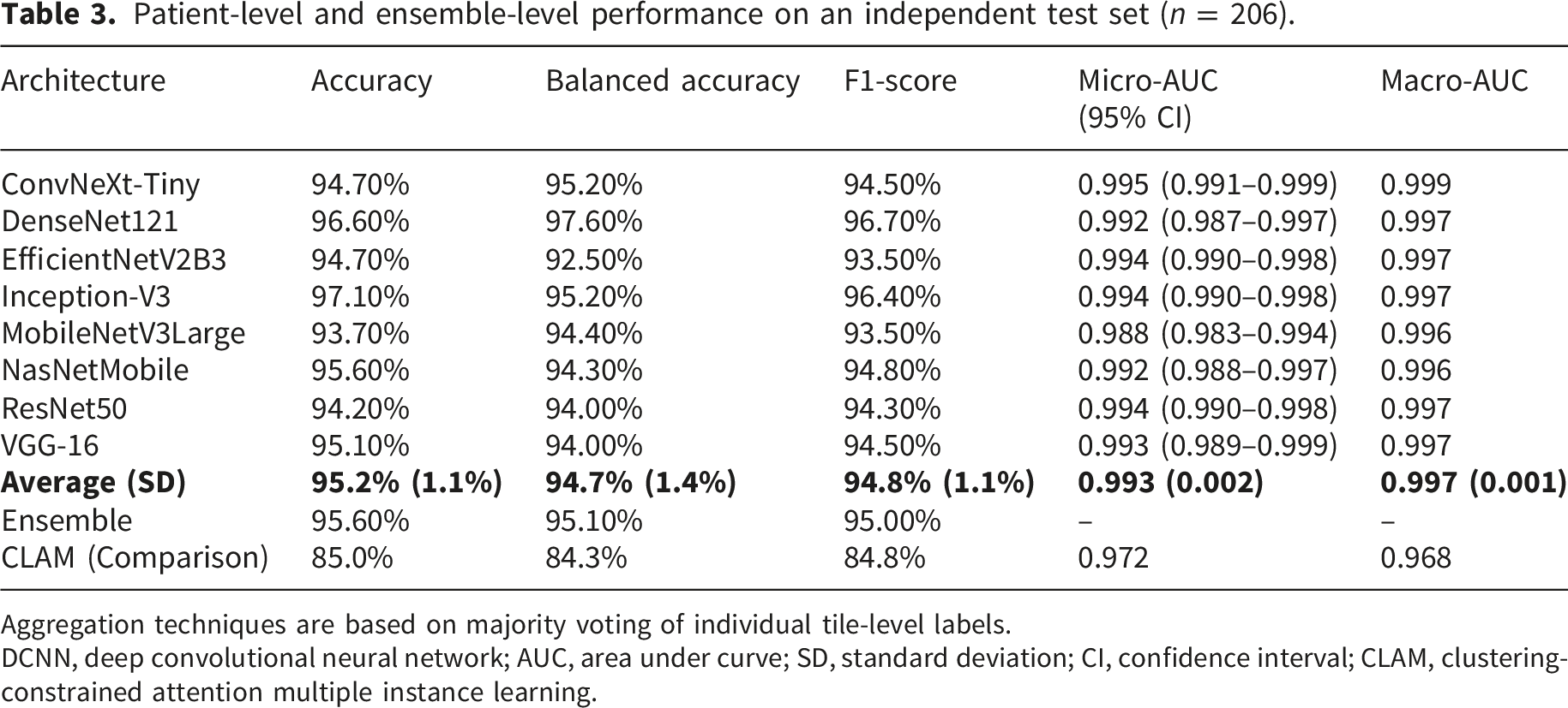
Aggregation techniques are based on majority voting of individual tile-level labels.

DCNN, deep convolutional neural network; AUC, area under curve; SD, standard deviation; CI, confidence interval; CLAM, clustering-constrained attention multiple instance learning.

In terms of tile-level predictions, each of the 200 tiled images from a single patient was treated independently. Average accuracy, balanced accuracy, F1-score, and micro-averaged AUC achieved 88.8%, 88.1%, 87.7%, and 0.986, respectively (Table 2). Among the eight selected models, ConvNeXt-Tiny achieved the best performance, with 91.5% accuracy, 91.7% balanced accuracy, 90.9% F1-score, and 0.991 micro-averaged AUC. Generally, the balanced accuracies (average: 88.1%) were slightly inferior to accuracies (average: 88.8%), reflecting a mild bias towards the larger classes.

At the patient level, averaged accuracy, balanced accuracy, F1-score, and micro-averaged AUC attained 95.2%, 94.7%, 94.8%, and 0.993, respectively (Table 3). Our aggregation method significantly improved the patient-level accuracy of all models compared with the tile-level (p < 0.01). ConvNeXt-Tiny reached the highest AUC (micro-averaged AUC = 0.995), whereas Inception-V3 and DenseNet121 models had the highest accuracy, attaining 97.1% and 96.6%, respectively. DenseNet121 achieved 97.6% balanced accuracy and a 96.7% F1-score, which were both slightly superior to those of the Inception-V3. These results indicate that DensNet121 possesses less bias toward larger diseases during prediction. Through confusion matrices (Figure 2; Supplemental Figure 1), it can be noted that the sensitivity of AML was impaired. When inspecting the ROIs which were incorrectly predicted, we found many of them improperly illuminated.

Pooling predictions from eight architectures together for a patient, the ensemble model reached only slightly better results than the average patient-level statistics, with accuracy 95.6% vs. 95.2%, balanced accuracy 95.1% vs. 94.7%, and F1-score 95.0% vs. 94.8% (Table 3).

Ancillary analyses

To validate our methodology, three ancillary experiments were conducted. Firstly, we compared our patient-level performance with the revolutionary attention-based CLAM model as a comparison study. With learning rate set to 0.0001, the training process stopped prematurely at the 104^th epoch without improving validation loss. On the same test set, the CLAM model was inferior to ours, reaching accuracy, balanced accuracy, F1 score, and micro-averaged AUC of 85.0%, 84.3%, 84.8%, and 0.972, respectively (Table 3).

Secondly, we replaced the quality-based ROI selection with random tile image sampling as an ablation study of the pipeline’s first stage. An ablated classification model based on DenseNet121 architecture was trained with the same configurations, and it attained accuracy, balanced accuracy, F1 score, and micro-averaged AUC of 89.3%, 88.5%, 89.5%, and 0.988, respectively on the random tiles from the same test set patients (Supplemental Table 3). The inferior results demonstrated the effectiveness of the ROI selection stage.

Thirdly, we evaluated the model’s robustness across high- and low-neoplastic cell percentage groups. After dichotomization, the thresholds for subgroup stratification was 80% and 60% for AML blast percentage and MM plasma cell percentage, respectively. In AML, the patient-level accuracy was 93.3% in the high-blast group and 90.9% in the low-blast group, while in MM, the accuracy was 96.2% in the high-plasma cell group and 93.8% in the low-plasma cell group. All AUCs of the four groups were greater than 0.96, especially above 0.999 for MM (Supplemental Table 4). These findings suggest that our classification model preserved robust discriminative performance across cell-percentage subgroups.

External validation

Given its small bias towards large classes and short inference time, the second stage model based on DenseNet121 was selected as our final model for external validation. On the KVGH cohort, 6 ALL, 51 AML, and 17 MM WSIs underwent cropping and ROI selection by our first-stage model. Our final second-stage model attained patient-level accuracy, balanced accuracy, and micro-averaged AUC of 83.8%, 84.6%, and 0.961, respectively, demonstrating decent performance and little bias to large classes. For SN-AM preprocessed ROIs, tile-level accuracy, balanced accuracy, and micro-averaged AUC were 86.7%, 86.7%, and 0.974, respectively without first-stage ROI quality control. These results showed the potential of our DCNN models to generalize to all bone marrow aspirate images.

Visual explanation of an example model

We generated grad-CAMs upon two CNN layers: the penultimate layer and an intermediate layer, to obtain a coarse view of the model’s perception at different depths within the backbone CNN. Five tiles of different diseases were selected to perform grad-CAM visualization, as shown in Figure 3(a–e). While grad-CAM on the intermediate layer revealed higher salience on nuclei borders or cytoplasm depending on class labels, those on the penultimate layer manifested consistency between salience and cell distribution. These results suggest that the DenseNet121 model successfully identified diagnostic image features within the regions occupied by nucleated cells. Furthermore, WSI-level scatter plots revealed that ROIs randomly selected by our quality assessment model were distributed in regions with moderate cellular density (Figure 4). We also noted that misclassified ROIs were often located in ROI-sparse areas, although many of them were canceled out during patient-level aggregation.

Figure 3.

Examples of grad-CAM of the selected DenseNet121 model. Rows (a–e) present five ROIs selected from the test set of classes ALL, AML, CML, lymphoma, and MM, respectively. In each row, the left panel displays the original tile image; the middle panel displays grad-CAM on an intermediate layer, revealing higher salience (shown in red) on nuclei borders or cytoplasm; the right panel displays grad-CAM on the penultimate layer, which is the layer just before the classifier network, showing spatial consistency between salience and cell distribution.

Figure 4.

Examples of WSI-level saliency maps of the selected DenseNet121 model. Rows (a–e) present five WSIs selected from the test set of classes ALL, AML, CML, lymphoma, and MM, respectively. In each row, the left panel shows the scatter plot of 200 ROIs on the WSI thumbnail image, where colors of red, orange, yellow, green, and light blue represent the tile is predicted to be ALL, AML, CML, lymphoma, and MM, respectively. In the right panel, a saliency map combining density and probability for correctness was superimposed onto the WSI thumbnail image, providing intuition for areas to start with during manual review. Generally, ROIs are in areas with uniformly-distributed cells or at the border of dense cell clumps, while correctly-predicted ROIs primarily reside in areas where ROIs are dense. ALL, acute lymphoblastic leukemia; AML, acute myeloblastic leukemia; CML, chronic myelocytic leukemia; MM, multiple myeloma; ROI, region of interest; WSI, whole slide image.

Discussion

In this article, we present a two-stage pipeline to differentiate among different leukemic diseases and lymphoma using digitized, Wright–Giemsa-stained WSIs without requirement for manual ROI placement. Such a design enables development of a fully automated diagnostic tool with visualization of relevant slide regions, which expedites the diagnosis workflow without sacrificing accuracy especially when hematopathologists are preoccupied or scarce. To the best of our knowledge, our approach achieved the highest accuracy among the few published methods performing the same task. We also prove the feasibility of both a DCNN-based ROI selection method and an instance-based aggregation approach to yield a WSI-level prediction. Our WSI dataset comprises 1,022 high-resolution bone marrow aspirate smears and more than 24 million tiled images, which is also the largest cohort used to train hematologic neoplasm classifiers.

Through literature review, we summarized that strategies for processing a WSI can be divided into two types: ROI selection, which identifies relevant tiled images prior to formal classification, and multiple instance learning (MIL), which aggregates either instance labels or feature vectors generated from all ROIs. The International Council for Standardization in Hematology (ICSH) recommends first identifying areas of well-spread marrow smears and then assessing cytology in these areas under higher magnification.⁵ Such a standardization provides a rationale for our ROI selection stage, in which a DCNN is trained to identify tiles with adequate cell distribution. Without quality assessment model, the second stage classifier would have been trained on 14.8 million tiles, consuming 121 times more resources. Most importantly, ROI selection precluded noninformative patches from interfering with classification, as demonstrated by the ablation study. Much in the same way, Kockwelp et al.²⁴ trained a cell-level grading network with only 1,506 manually annotated tiles and reduced up to 99.9% of labeling effort without sacrificing their validation accuracy (Table 4).

Table 4.

Comparison among strategies to automatically process whole slide images in different studies of hematologic neoplasm classification.

Study	Objective	Total valid dataset	ROI selection method	MIL method	Reported results
Kockwelp et al.²⁸	Predict AML ELN2017 label	153 BM smears	Identify valid cells from auto-segmented cells	Embedding-based	Accuracy = 0.764
	Predict AML NPM1 status				Accuracy = 0.834
	Predict AML FLT3 status				Accuracy = 0.836
Wang et al.²⁹	Classify AML, CML, ALL, CLL, and MM	129 BM smears	None	Embedding-based, attention-based	(5-fold CV)
					Average accuracy = 0.900
					Average AUC = 0.979
Mu et al.⁴⁵	Classify leukemia, LPD, PCN, and MDS	556 BM smears	Identify valid cells with YOLO DCNN	Embedding-based, attention-based	(5-fold CV)
Mu et al.⁴⁵	Classify leukemia, LPD, PCN, and MDS	556 BM smears	Identify valid cells with YOLO DCNN	Embedding-based, attention-based	Average F1-score = 0.566
Syrykh et al.⁴⁶	Identify follicular lymphoma from follicular hyperplasia	378 lymph node sections	Remove tiles covered with < 50% tissue	Instance-based, prediction averaging	AUC = 0.990
Our study	Classify ALL, AML, CML, lymphoma, and MM	1,022 BM smears	Identify high quality tiles	Instance-based, majority voting	Accuracy = 0.952
					Micro-AUC = 0.993
					F1-score = 0.948

ALL, acute lymphoblastic leukemia; AML, acute myeloblastic leukemia; CML, chronic myelocytic leukemia; MM, multiple myeloma; LPD, lymphoproliferative disorder; PCN, plasma cell neoplasm; MDS, myelodysplastic syndrome; ELN, European LeukemiaNet; BM, bone marrow; ROI, region of interest; MIL, multiple instance learning; CV, cross validation; AUC, area under curve; DCNN, deep convolutional neural network.

Inferring a single label from a bag of input instances, the second strategy, MIL, has been particularly useful in medical image diagnosis¹⁰ and can be conducted in two manners. Instance-based MIL aggregates the prediction results of all input instances, while embedding-based MIL aggregates feature vectors of all input instances before deriving a final prediction.^49,50 As demonstrated by Wang et al.²⁵ and Mu et al.,⁵¹ embedding-based MIL can be further integrated with attention network architecture to impose greater weights on relevant feature vectors, compensating for the absence of ROI selection. On the other hand, instance-based MIL provides an intuitive way to identify crucial ROI instances, but it also raises concerns about increased error rate when many noninformative instances are present.⁵⁰ Syrykh et al.⁵² calculated the average of all instance predictions without ROI selection and justified their method with spatial constancy of lymph node specimen slides. In comparison, our first-stage model selected 200 most informative ROIs and allowed majority voting to significantly improve patient-level accuracy by 6.4% (p < 0.05), eventually outperforming embedding-based MIL methods such as CLAM. Similar performance gains after aggregation were also reported by previous studies on multiclass classification,^18,43,53 but only our pipeline successfully adopted an automatic ROI selection model.

With an aim to explore the full potential of our algorithm, we applied transfer learning on eight popular DCNN architectures and compared their performance with one another. In terms of AUC, ConvNeXt-Tiny achieved the best performance, yet its accuracy, balanced accuracy, and F1-score were surpassed by DenseNet121 and Inception-V3 on the patient level. A possible explanation would be that DenseNet121 and Inception-V3 made more mistakes that, nonetheless, were concentrated in fewer WSIs. We also noted that our ensemble model did not improve the performance much. Our results suggest that eight DCNN classifiers tended to agree on each WSI prediction even when there was misjudgment, thereby reducing the benefit of ensemble. This phenomenon inspired us to develop an algorithm with an uncertainty level output, with which models can report an uncertain prediction rather than directly misclassify.⁵²

Finally, we address the visual interpretation of our pipeline in two levels. Several visualization methods have been proposed to evaluate the behavior of DCNN across an input image, among which occlusion sensitivity analysis has high local faithfulness but is also computationally inefficient.⁵⁴ In this study, we applied grad-CAM, which requires only one complete forward propagation and partial backpropagation for a single input. In addition to validating DCNN models, these color maps may potentially identify relevant microstructures that were previously unknown. On the WSI level, we mapped the locations of 200 ROIs along with their predicted classes on their corresponding WSI thumbnail image, creating a whole slide heatmap emphasizing relevant areas in a resolution finer than that of Syrykh’s study.⁵² We believe such visualization assists hematopathologists in rapidly selecting areas to examine if manual review becomes necessary.

Despite the satisfactory performance in WSI multiclass classification, our study has several limitations. First, the quality assessment model was not trained using manually removed out-of-focus areas, which may limit its ability to exclude blurred or poorly focused tiles. Second, the accuracies on external cohort were remained inferior to those observed in the internal test set. Staining variability is a well-recognized contributor to domain shift in computational pathology,⁵⁵ and additional external WSI datasets acquired using diverse staining and scanning protocols are required to improve model generalizability. In addition, clinically relevant variables, such as impaired renal function in MM⁵⁶ and younger age in ALL,⁵⁷ were not incorporated into our classification model. Finally, our study included only high-magnification image tiles to preserve intracellular morphologic details. To fully exploit the information available in WSIs, tiles acquired at lower magnifications could also be incorporated to provide complementary features such as overall cellularity and architectural context.

Our plan for future research encompasses three directions. First, to develop more robust and generalizable models, it is necessary to expand the WSI database to include samples from multiple institutes, across diverse racial populations, and with more comprehensive clinical information. Next, we aim to design novel neural network architectures or adopt vision–language models capable of integrating clinical variables with image features, with the goal of achieving improved performance while reducing computational burden. Finally, beyond disease classification, we intend to explore predictive modeling of molecular diagnoses and treatment response using baseline imaging and clinical data. Such advances may not only accelerate the diagnostic process but also provide clinically actionable insights to support personalized treatment planning.

Conclusion

In summary, our two-stage pipeline successfully classifies whole slide BM aspirate smears into multiple hematologic neoplasms with high average accuracy and AUC. Our approach benefits clinical physicians in differential diagnosis and treatment planning at initial encounter, and aids hematopathologists in identifying relevant areas and microstructures. With further studies, our algorithm using ROI selection and instance aggregation has the potential to classify more advanced tasks, including myelodysplastic diseases and lymphoma subtypes.

Supplemental material

Supplemental material - Classification of hematologic malignancies from whole-slide bone marrow aspirates using a two-stage deep convolutional neural network pipeline

Supplemental material for Classification of hematologic malignancies from whole-slide bone marrow aspirates using a two-stage deep convolutional neural network pipeline by Hung-Ruei Chen, Yao-Chung Liu, Chiu-Mei Yeh, Cheng-Kuan Lin, Tzu-Ya Chien, Ying-Chung Hong, Chia-Jen Liu and Kun-Hsing Yu in Digital Health.

Footnotes

ORCID iDs

Hung-Ruei Chen

Chia-Jen Liu

Ethical considerations

This study has received approval from the Institutional Review Board at Taipei Veterans General Hospital, affirming its compliance with ethical research standards. All methods for the study were performed in accordance with relevant guidelines and regulations of Taipei Veterans General Hospital in Taiwan. The Taipei Veterans General Hospital ethical committee waived the informed consent form.

Author contributions

Hung-Ruei Chen: Conceptualization, Methodology, Software, Validation, Formal analysis, Investigation, Writing - Original Draft, Visualization. Yao-Chung Liu: Validation, Resources, Data curation. Chiu-Mei Yeh: Validation, Formal analysis, Resources, Data curation, Writing - Review & Editing. Cheng-Kuan Lin: Validation, Writing - Review & Editing. Tzu-Ya Chien: Validation, Writing - Review & Editing. Ying-Chung Hong: Validation. Chia-Jen Liu: Conceptualization, Methodology, Software, Validation, Formal analysis, Resources, Data curation, Writing - Review & Editing, Supervision, Project administration, Funding acquisition. Kun-Hsing Yu: Conceptualization, Methodology, Validation, Resources, Writing - Review & Editing.

Funding

The authors disclosed receipt of the following financial support for the research, authorship, and/or publication of this article: This study was supported by grants from Taipei Veterans General Hospital [grant numbers V113C-055, V114C-214, and V115C-044]; the Ministry of Science and Technology [grant numbers MOST 111-2314-B-A49-034-, NSTC 113-2314-B-A49-027-, and NSTC 114-2314-B-A49-054-]; the Yen Tjing Ling Medical Foundation; the Taiwan Clinical Oncology Research Foundation; and the Melissa Lee Cancer Foundation. The funding sources had no role in the study design or conduct, or in the decision to submit it for publication.

Declaration of conflicting interests

The authors declared no potential conflicts of interest with respect to the research, authorship, and/or publication of this article.

Data Availability Statement

The datasets used and analyzed during the current study are available from the corresponding author upon reasonable request.*

Supplemental material

Supplemental material for this article is available online.

References

Zhang

Wang

, et al. Global burden of hematologic malignancies and evolution patterns over the past 30 years. Blood Cancer Journal 2023; 13: 82. https://doi.org/10.1038/s41408-023-00853-3

Siegel

Kratzer

Giaquinto

, et al. Cancer statistics, 2025. CA Cancer J Clin 2025; 75: 10–45, 20250116. https://doi.org/10.3322/caac.21871

Falini

Martelli

. Comparison of the International Consensus and 5th WHO edition classifications of adult myelodysplastic syndromes and acute myeloid leukemia. American Journal of Hematology 2023; 98: 481–492. https://doi.org/10.1002/ajh.26812

Bedu-Addo

Ampem Amoako

Bates

. The role of bone marrow aspirate and trephine samples in haematological diagnoses in patients referred to a teaching hospital in Ghana. Ghana Med J 2013; 47: 74–78.

Lee

Erber

Porwit

, et al. ICSH guidelines for the standardization of bone marrow specimens and reports. International Journal of Laboratory Hematology 2008; 30: 349–364. https://doi.org/10.1111/j.1751-553X.2008.01100.x

Kanakis

Mirza

. Demystifying the Bone Marrow Biopsy: A Hematopathology Primer. https://www.hematology.org/education/trainees/fellows/hematopoiesis/2021/demystifying-the-bone-marrow-biopsy-a-hematopathology-primer (2021, accessed February 04 2026).

Khoury

Solary

Abla

, et al. The 5th edition of the World Health Organization Classification of Haematolymphoid Tumours: Myeloid and Histiocytic/Dendritic Neoplasms. Leukemia 2022; 36: 1703–1719. https://doi.org/10.1038/s41375-022-01613-1

Arber

Orazi

Hasserjian

, et al. International Consensus Classification of Myeloid Neoplasms and Acute Leukemias: integrating morphologic, clinical, and genomic data. Blood 2022; 140: 1200–1228, 2022/06/30. https://doi.org/10.1182/blood.2022015850

Tayebi

Dehkharghanian

, et al. Automated bone marrow cytology using deep learning to generate a histogram of cell types. Communications Medicine 2022; 2: 45. https://doi.org/10.1038/s43856-022-00107-6

10.

Srisuwananukorn

Salama

Pearson

. Deep learning applications in visual data for benign and malignant hematologic conditions: a systematic review and visual glossary. Haematologica 2023; 108: 1993–2010, 20230801. https://doi.org/10.3324/haematol.2021.280209

11.

Ghaderzadeh

Asadi

Hosseini

, et al. Machine Learning in Detection and Classification of Leukemia Using Smear Blood Images: A Systematic Review. Scientific Programming 2021; 2021: 9933481. https://doi.org/10.1155/2021/9933481

12.

Loey

Naman

Zayed

. Deep Transfer Learning in Diagnosing Leukemia in Blood Cells. Computers 2020; 9: 29. https://doi.org/10.3390/computers9020029

13.

Anilkumar

Manoj

Sagi

. Automated detection of leukemia by pretrained deep neural networks and transfer learning: A comparison. Med Eng Phys 2021; 98: 8–19, 20211013. https://doi.org/10.1016/j.medengphy.2021.10.006

14.

Abunadi

Senan

. Multi-Method Diagnosis of Blood Microscopic Sample for Early Detection of Acute Lymphoblastic Leukemia Based on Deep Learning and Hybrid Techniques. Sensors 2022; 22: 1629. https://doi.org/10.3390/s22041629

15.

Eckardt

J-N

Schmittmann

Riechert

, et al. Deep learning identifies Acute Promyelocytic Leukemia in bone marrow smears. BMC Cancer 2022; 22: 201. https://doi.org/10.1186/s12885-022-09307-8

16.

Wen

, et al. AMLnet, A deep-learning pipeline for the differential diagnosis of acute myeloid leukemia from bone marrow smears. Journal of Hematology & Oncology 2023; 16: 27. https://doi.org/10.1186/s13045-023-01419-3

17.

Eckardt

J-N

Middeke

Riechert

, et al. Deep learning detects acute myeloid leukemia and predicts NPM1 mutation status from bone marrow smears. Leukemia 2022; 36: 111–118. https://doi.org/10.1038/s41375-021-01408-w

18.

Achi

Belousova

Chen

, et al. Automated Diagnosis of Lymphoma with Digital Pathology Images Using Deep Learning. Ann Clin Lab Sci 2019; 49: 153–160.

19.

Claro

Vogado

Veras

, et al. Convolution Neural Network Models for Acute Leukemia Diagnosis. In: 2020 International Conference on Systems, Signals and Image Processing (IWSSIP), Niterói, Rio de Janeiro, Brazil, 1–3 July 2020, pp. 63–68.

20.

Manescu

Narayanan

Bendkowski

, et al. Detection of acute promyelocytic leukemia in peripheral blood and bone marrow with annotation-free deep learning. Scientific Reports 2023; 13: 2562. https://doi.org/10.1038/s41598-023-29160-4

21.

Ahmed

Yigit

Isik

, et al. Identification of Leukemia Subtypes from Microscopic Images Using Convolutional Neural Network. Diagnostics (Basel) 2019; 9: 20190825. https://doi.org/10.3390/diagnostics9030104

22.

Huang

Guang

, et al. AML, ALL, and CML classification and diagnosis based on bone marrow cell morphology combined with convolutional neural network: A STARD compliant diagnosis research. Medicine 2020; 99: e23154. https://doi.org/10.1097/MD.0000000000023154

23.

Amin

Mori

Itoh

. A validation study of whole slide imaging for primary diagnosis of lymphoma. Pathology International 2019; 69: 341–349. https://doi.org/10.1111/pin.12808

24.

Kockwelp

Thiele

Kockwelp

, et al. Cell Selection-based Data Reduction Pipeline for Whole Slide Image Analysis of Acute Myeloid Leukemia. In: 2022 IEEE/CVF Conference on Computer Vision and Pattern Recognition Workshops (CVPRW), New Orleans, LA, USA, 19-20 June 2022. IEEE Computer Society, 2022, pp. 1824–1833.

25.

Wang

Wei

X-L

C-X

, et al. Efficient and Highly Accurate Diagnosis of Malignant Hematological Diseases Based on Whole-Slide Images Using Deep Learning. Frontiers in Oncology 2022; 12: 879308, Original Research. https://doi.org/10.3389/fonc.2022.879308

26.

Swerdlow

Campo

Harris

, et al. WHO classification of tumours of haematopoietic and lymphoid tissues. International agency for research on cancer, 2008.

27.

Weinzierl

Arber

. Bone marrow evaluation in new-onset pancytopenia. Human Pathology 2013; 44: 1154–1164. https://doi.org/10.1016/j.humpath.2012.10.006

28.

Ullah

Khan

Qureshi

. Etiological Spectrum of Bone Marrow Biopsy in Patients With Pancytopenia. Cureus 2024; 16: e73138. https://doi.org/10.7759/cureus.73138

29.

Goode

Gilbert

Harkes

, et al. OpenSlide: A vendor-neutral software foundation for digital pathology. J Pathol Inform 2013; 4: 27, 20130927. https://doi.org/10.4103/2153-3539.119005

30.

Tampu

Eklund

Haj-Hosseini

. Inflation of test accuracy due to data leakage in deep learning-based classification of OCT images. Scientific Data 2022; 9: 580. https://doi.org/10.1038/s41597-022-01618-6

31.

Khalifa

Loey

Mirjalili

. A comprehensive survey of recent trends in deep learning for digital images augmentation. Artificial Intelligence Review 2022; 55: 2351–2377. https://doi.org/10.1007/s10462-021-10066-4

32.

Simonyan

Zisserman

. Very Deep Convolutional Networks for Large-Scale Image Recognition. arXiv:1409.1556. https://doi.org/10.48550/arXiv.1409.1556

33.

Szegedy

Vanhoucke

Ioffe

, et al. Rethinking the Inception Architecture for Computer Vision. In: 2016 IEEE Conference on Computer Vision and Pattern Recognition (CVPR), Las Vegas, NV, USA, 27–30 June 2016, pp. 2818–2826.

34.

Zhang

Ren

, et al. Deep Residual Learning for Image Recognition. In: 2016 IEEE Conference on Computer Vision and Pattern Recognition (CVPR), Las Vegas, NV, USA, 27–30 June 2016, pp. 770–778.

35.

Huang

Liu

Maaten

LVD

, et al. Densely Connected Convolutional Networks. In: 2017 IEEE Conference on Computer Vision and Pattern Recognition (CVPR), Honolulu, HI, USA, 21–26 July 2017, pp. 2261–2269.

36.

Howard

Sandler

Chen

, et al. Searching for MobileNetV3. In: 2019 IEEE/CVF International Conference on Computer Vision (ICCV), Seoul, South Korea, 27 Oct–2 Nov. 2019, pp. 1314–1324.

37.

Zoph

Vasudevan

Shlens

, et al. Learning Transferable Architectures for Scalable Image Recognition. In: 2018 IEEE/CVF Conference on Computer Vision and Pattern Recognition, Salt Lake City, UT, USA, 18–23 June 2018, pp. 8697–8710.

38.

Liu

Mao

, et al. A ConvNet for the 2020s. In: 2022 IEEE/CVF Conference on Computer Vision and Pattern Recognition (CVPR), New Orleans, LA, USA, 18–24 June 2022, pp. 11966–11976.

39.

Tan

. EfficientNetV2: Smaller Models and Faster Training. In: In: Marina M, Tong Z (Eds)., Proceedings of the 38th International Conference on Machine Learning. Proceedings of Machine Learning Research (eds). Marina

Tong

. Virtual Event PMLR, 2021, pp. 10096–10106.

40.

Leevy

Khoshgoftaar

Bauder

, et al. A survey on addressing high-class imbalance in big data. Journal of Big Data 2018; 5: 42. https://doi.org/10.1186/s40537-018-0151-6

41.

Ganaie

Malik

, et al. Ensemble deep learning: A review. Engineering Applications of Artificial Intelligence 2022; 115: 105151. https://doi.org/10.1016/j.engappai.2022.105151

42.

Grandini

Bagli

Visani

. Metrics for multi-class classification: an overview. arXiv preprint arXiv:200805756 2020. https://doi.org/10.48550/arXiv.2008.05756

43.

Steinbuss

Kriegsmann

Zgorzelski

, et al. Deep Learning for the Classification of Non-Hodgkin Lymphoma on Histopathological Images. Cancers 2021; 13: 2419. https://doi.org/10.3390/cancers13102419

44.

Zou

O’Malley

Mauri

. Receiver-Operating Characteristic Analysis for Evaluating Diagnostic Tests and Predictive Models. Circulation 2007; 115: 654–657. https://doi.org/10.1161/CIRCULATIONAHA.105.594929

45.

Williamson

DFK

Chen

, et al. Data-efficient and weakly supervised computational pathology on whole-slide images. Nature Biomedical Engineering 2021; 5: 555–570. https://doi.org/10.1038/s41551-020-00682-w

46.

Gupta

. SN-AM Dataset: White Blood Cancer Dataset of B-ALL and MM for Stain Normalization. 1st ed. The Cancer Imaging Archive, 2019.

47.

Reinhard

Adhikhmin

Gooch

, et al. Color transfer between images. IEEE Computer Graphics and Applications 2001; 21: 34–41. https://doi.org/10.1109/38.946629

48.

Selvaraju

Cogswell

Das

, et al. Grad-CAM: Visual Explanations from Deep Networks via Gradient-Based Localization. In: 2017 IEEE International Conference on Computer Vision (ICCV), 22–29 Oct. 2017. IEEE Computer Society, pp. 618–626.

49.

Ilse

Tomczak

Welling

. Attention-based Deep Multiple Instance Learning. In: Proceedings of the 35th International Conference on Machine Learning. Proceedings of Machine Learning Research (eds. Jennifer

Andreas

), PMLR, 2018, pp. 2127–2136.

50.

Eliceiri

. Dual-stream Multiple Instance Learning Network for Whole Slide Image Classification with Self-supervised Contrastive Learning. In: Proceedings of the IEEE/CVF Conference on Computer Vision and Pattern Recognition (CVPR), Virtual, June 24, 2021, pp. 14318–14328.

51.

Tizhoosh

Dehkharghanian

, et al. Whole slide image representation in bone marrow cytology. Computers in Biology and Medicine 2023; 166: 107530. https://doi.org/10.1016/j.compbiomed.2023.107530

52.

Syrykh

Abreu

Amara

, et al. Accurate diagnosis of lymphoma on whole-slide histopathology images using deep learning. npj Digital Medicine 2020; 3: 63. https://doi.org/10.1038/s41746-020-0272-0

53.

Yang

Qin

, et al. Efficient diagnosis of hematologic malignancies using bone marrow microscopic images: A method based on MultiPathGAN and MobileViTv2. Comput Methods Programs Biomed 2023; 237: 107583, 20230509. https://doi.org/10.1016/j.cmpb.2023.107583

54.

Uchiyama

Sogi

Niinuma

, et al. Visually explaining 3D-CNN predictions for video classification with an adaptive occlusion sensitivity analysis. In: 2023 IEEE/CVF Winter Conference on Applications of Computer Vision (WACV). Waikoloa, HI, USA. IEEE 2023, pp. 1513–1522.

55.

Hetz

Bucher

T-C

Brinker

. Multi-domain stain normalization for digital pathology: A cycle-consistent adversarial network for whole slide images. Medical Image Analysis 2024; 94: 103149. https://doi.org/10.1016/j.media.2024.103149

56.

Rajkumar

Dimopoulos

Palumbo

, et al. International Myeloma Working Group updated criteria for the diagnosis of multiple myeloma. Lancet Oncol 2014; 15: e538–e548, 20141026. https://doi.org/10.1016/s1470-2045(14)70442-5

57.

Malard

Mohty

. Acute lymphoblastic leukaemia. Lancet 2020; 395: 1146–1162. https://doi.org/10.1016/s0140-6736(19)33018-1

Supplementary Material

Please find the following supplemental material available below.

For Open Access articles published under a Creative Commons License, all supplemental material carries the same license as the article it is associated with.

For non-Open Access articles published, all supplemental material carries a non-exclusive license, and permission requests for re-use of supplemental material or any part of supplemental material shall be sent directly to the copyright owner as specified in the copyright notice associated with the article.

0.66 MB

0.00 MB