Optimizing deep learning models to combat amyotrophic lateral sclerosis (ALS) disease progression

Abstract

Objective

Amyotrophic lateral sclerosis (ALS), a devastating neurodegenerative disease, poses a significant challenge for targeted treatment development. Accurate prediction of its progression is crucial for this endeavor.

Methods

This study investigated deep learning methods for ALS progression prediction using the publicly available PRO-ACT dataset. Initially, machine learning models (XGBoost, LightGBM) and a deep learning sequential model were evaluated with default parameters, using R-squared (R2) and Root Mean Squared Error (RMSE) as performance metrics.

Results

Notably, the deep learning model demonstrated superior predictive performance with default settings (RMSE: 4.565, R2: 0.716), followed by XGBoost (RMSE: 4.625, R2: 0.709) and LightGBM (RMSE: 4.596, R2: 0.716). Subsequently, hyperparameter optimization significantly enhanced the deep learning model's performance, achieving the highest prediction accuracy (RMSE: 4.511, R2: 0.718). Slight improvements were also observed for XGBoost (RMSE: 4.532, R2: 0.715) and LightGBM (RMSE: 4.551, R2: 0.716). Furthermore, the optimized XGBoost model demonstrated exceptional classification performance in distinguishing between bulbar and limb onset ALS, with a sensitivity of 100%, specificity of 97.44%, accuracy of 97.96%, F1-score of 95.96%, Matthews Correlation Coefficient (MCC) of 94.12%, and an Area Under the Curve (AUC) of 0.9550. Feature importance analysis with optimized XGBoost identified ZBTB2P1 as the most influential feature, followed by RNF181, with WASH9P being the least influential among the top eight.

Conclusions

These findings convincingly demonstrate the potential of optimized XGBoost and deep learning for ALS progression prediction and classification, particularly with optimized parameters. This approach offers significant potential for early risk stratification, personalized treatment planning, enhanced prognostic communication, diagnostic support, streamlined disease monitoring, and improved clinical decision-making, ultimately contributing to better patient outcomes and potentially reducing ALS-related mortality.

Introduction

Occurring at an estimated rate of 2–3 cases per 100,000 individuals in Europe, ¹ 1–2 per 100,000 in the United States (with a prevalence of 4–6 per 100,000), and even lower in Eastern and Southern Asia (0.8 and 0.7 per 100,000 respectively), ² Amyotrophic lateral sclerosis (ALS) is a devastating neurodegenerative disease characterized by the hallmark degeneration of both upper (originating in the brain and descending to the brainstem and spinal cord) and lower motor neurons (connecting the brainstem and spinal cord to muscles). Several cellular and molecular mechanisms, including disrupted calcium homeostasis, misfolded protein accumulation, glutamate excitotoxicity, prion-like spreading, and RNA processing defects, contribute to the cascade of cellular damage leading to motor neuron loss.^1–3 Despite growing evidence suggesting a complex interplay between genetic and environmental factors in ALS pathogenesis,^4,5 the precise pathophysiological processes underlying the disease remain elusive.

The ALS also known as Lou Gehrig's disease, is a progressive neurodegenerative disease affecting nerve cells in the brain and spinal cord.^6–9 While ALS typically progresses at different rates in different individuals and can affect various muscles and body systems, its progression generally follows similar patterns.^9–11 Initial symptoms often involve weakness or twitching in the arms or legs, which may then spread throughout the body. As the disease advances, muscle weakness increases, making movement, speech, swallowing, and breathing increasingly difficult. Progression is typically measured by the extent of muscle weakness and functional impairment. Several factors, including age of onset, site of onset, ALS type (e.g Bulbar vs. Limb Onset), and pre-existing medical conditions, can influence the rate of progression. While most cases progress slowly over several years, rapid progression is possible.^12–16 Although most individuals with ALS succumb to respiratory failure within 3 to 5 years of onset, some survive considerably longer. Currently, there is no cure for ALS, but. treatments such as medication, physical therapy, and respiratory support can help manage symptoms and improve quality of life.

Approximately 70% of ALS patients experience limb-onset symptoms, while the remaining 30% present with bulbar-onset symptoms, affecting speech and swallowing. The prognosis for ALS is generally poor, with most patients succumbing to respiratory failure within 3 to 5 years of symptom onset.^1–3 Diagnosing ALS is challenging due to its heterogeneous nature, resulting from factors such as the combined involvement of upper and lower motor neurons, unpredictable disease progression, and variable onset locations. ¹⁷ Accurate diagnosis and disease management require a comprehensive approach, integrating clinical evaluation, electrophysiological tests, and imaging techniques. These factors, including body mass index, ¹⁸ gender, affected body regions, muscle weakness, vital capacity, ¹⁹ Riluzole therapy, ²⁰ onset site, ²¹ executive dysfunction or comorbid frontotemporal dementia (FTD), El Escorial categorization,^1–3 functional disability ²² and symptom onset age, are also important prognostic indicators.

Like many neuromuscular conditions, ALS is diagnosed as a condition of exclusion, and as the name suggests, some optimal level of diagnostic certainty has to be achieved through applying criteria like El Escorial and Airlie House. ¹⁵ These guidelines measure the distribution and severity of both upper and lower motor neuron signs. However, these are often slow and cumbersome owing to the variability of ALS and its disease progression history. This calls for the ALS diagnoses predictive biomarkers to improve diagnostic accuracy, patient stratification, and prognostic capabilities.”

Depending on the advancements in the sickness, different systems are used to track ALS stages, such as in ALSFRS-R, which is the ALS Functional Rating Scale Revised. The rating scale covers bulbar (swallowing and speech), respiratory, and gross motor (walking) functions, with 12 items and a rating from 0–4. The King system modifies ALSFRS-R by using its domains to determine which parts of the body is affected and the chances of nutritional or respiratory complications. ²³ So does the “Loss of functional autonomy” of the Milano-Torino system, that is the MITOS system, in the same domains as the ALSFRS. ²⁴ Although these systems are useful for tracking development, they reveal the need for better predictive models which can outline the anticipated journey of each patient. These models are crucial to improve clinical trial designs by making forecasts, grouping patients, and possibly utilizing virtual control arms, which optimizes care for this multifaceted disease. ²⁵

Traditional ALS prognostic research has primarily utilized conventional statistical methods, including Cox regression, mixed-effects models, and Kaplan-Meier estimators. Although these earlier models, constrained by relatively strict data assumptions that limited their validity and processing capabilities, successfully identified key prognostic factors. These factors include body mass index, ¹⁸ gender, ²⁶ affected body regions, muscle weakness and vital capacity, ²⁷ Riluzole therapy, ²⁸ onset site, ²¹ executive dysfunction or comorbid frontotemporal dementia (FTD), ²⁹ functional disability, diagnostic delay, and age of symptom onset. ²⁹

Recently, machine learning (ML) models have garnered significant interest in ALS research. ³⁰ ML employs two primary approaches: supervised and unsupervised learning. The choice between these depends on the specific data characteristics and the research objective.

Unsupervised learning aims to discover patterns and structure within data without any predefined labels or feedback. ³¹ In contrast, supervised learning focuses on building models that map inputs to desired outputs using labeled training datasets. Several ML models have demonstrated effectiveness in ALS research, these incorporate Boosting techniques, neural networks (NN), k-nearest neighbors (k-NN), random forests (RF), support vector machines (SVM), Gaussian mixture models (GMM). Given the complex nature of ALS progression, research has focused on identifying potential prognostic biomarkers, including clinical, biological, imaging, and genetic factors. ³²

The strength of a prognostic model is in the attainment of accurately predicting the disease course. On a hypothetical front, ALS biomarkers would distinguish between heterogeneous phenotypes and stratify individuals according to rates of disease progression (slow progressors vs. fast progressors). ³³ Although clinical presentation has been the long-standing prognostic model, new literature discusses the combination of clinical information with imaging parameters. ³⁴ Multimodal research promises to revolutionize the prognosis and tailor treatments.

Several studies have demonstrated the benefit of integrating clinical and biological data to develop ALS prognostic models. ³⁵ This is achieved through the use of the complementary strengths of the two data sets to generate more informative and better predictions. Secondly, the pooled resource open-access ALS Clinical Trials (PRO-ACT) database has emerged as a valuable resource for most of the research studies to develop prognostic models.^25,35,36 The database provides a rich source of standardized clinical data, making it simple to develop and validate models. ALS prognostic modeling is generally targeted at predicting functional decline or survival. Predictions can be cast as classification problems, pre-specified classes, or regression problems, with continuous variables such as survival time or functional score. With two data sources and robust databases such as PRO-ACT, researchers are better positioned to develop more sophisticated prognostic models, which can enhance clinical decision-making and individualize patient management.

While traditional machine learning algorithms, such as SVM, KNN, and RF, have been applied in ALS studies, they can be limited in accuracy, particularly when default parameters are employed. More robust and adaptable approaches are needed for better prognostic functions.

Traditionally, supervised machine learning approaches in medical prognosis, including ALS, have relied on hand-crafted features, which tend to be time-consuming and labor-intensive to acquire. Selecting the most informative ones is a key challenge, and performance is limited by the quality and quantity of these hand-crafted features. Deep learning models offer an extremely appealing alternative by learning the features endogenously from data and circumventing the drudgery of manual feature design. Deep convolutional neural networks (CNNs) are especially widely known for their high performance across a wide range of applications, including large data processing and medical image processing.^37–41 CNNs utilize a stacked architecture, ⁴² where lower layers learn low-level features, which are then passed on to progressively higher layers in a hierarchical manner to learn progressively more complex patterns. This hierarchical architecture enables the model to learn complex relationships in the data, potentially to make better and more consistent prognostic predictions. ⁴³

Accurate prediction models have a central role to play in developing effective therapies against ALS, a progressive neurodegenerative condition. This study investigated the application of deep learning and machine learning models to predict ALS progression and onset type classification using the publicly available PRO-ACT dataset. After extensive preprocessing, XGBoost, LightGBM, and a 1D sequential deep learning model were initially compared on default hyperparameters. Next, hyperparameter tuning with grid search was applied for XGBoost and deep learning model for improving prediction accuracy. Feature importance analysis was also performed using the hyperparameter-optimized XGBoost model to identify predictive variables of importance. The results presented the deep learning model to possess better prediction accuracy, particularly following hyperparameter optimization. Moreover, the hyperparameter-optimized XGBoost model obtained a better performance for the classification of bulbar vs. limb onset ALS with an area under the curve (AUC) of 0.955. Feature importance analysis identified ZBTB2P1 to be the most important feature in the prediction model. These findings unveil the capability of optimized machine and deep learning techniques to predict ALS progression and onset type classification with accuracy. This method can have the ability to enhance early risk stratification, personalized treatment regimens, prognostic communication, diagnostic aid, reduction in disease surveillance, and ultimately optimize clinical decision-making and patient outcome in ALS.

Figure 1 illustrates the workflow for modeling ALS disease progression. ALS progression data were first preprocessed using data cleaning and augmentation techniques. A 10-fold cross-validation strategy was employed for training and testing. A one-dimensional convolutional neural network (1D CNN) sequential model was then trained and evaluated using both default parameters and optimized parameters identified through a grid search algorithm. Additionally, an ensemble model combining XGBoost, LightGBM, and a deep neural network (DNN) was implemented to assess the impact of a hybrid approach. Model performance was evaluated using R-squared and root mean squared error (RMSE) as metrics.

Figure 1.

Schematic diagram of ALS disease progression.

Materials and methods

Dataset

PRO-ACT ALS is a devastating neurodegenerative disease characterized by the progressive loss of voluntary muscle control, leading to paralysis, and difficulties with speech, swallowing, and breathing. While the prognosis is generally poor, with most patients succumbing to respiratory failure within 3 to 5 years of diagnosis and 90% within 10 years, advances in biotechnology offer hope for improved understanding and treatment. Initiatives like Answer ALS have generated unprecedented amounts of clinical and biological data from both ALS patients and healthy controls, providing valuable resources for researchers working to unravel the complexities of ALS and identify potential therapeutic targets.

Pre-processing

Data imputation

To meet the endemic challenge of missing data within the PRO-ACT ALS dataset, a systematic process of data cleaning was performed, using a range of imputation techniques appropriate to the longitudinal and clinical nature of the data. A thorough examination of missing data patterns was first conducted, employing visualizations to determine if missingness was at random or associated with particular factors. For longitudinal time-series measures, such as forced vital capacity (FVC), linear and spline interpolation were employed to fill gaps while preserving temporal relationships and conforming to the anticipated gradual decline in lung function. Cross-section clinical variables were imputed using K-nearest neighbors (KNN) and multiple imputation techniques, selected for their ability to model underlying data patterns and to allow imputation uncertainty. Domain-specific imputation, informed by clinical expertise, also ensured clinical plausibility and meaningfulness of imputed values. Indicators of missing values were generated to retain information on missingness, and sensitivity analyses were conducted to evaluate the impact of different imputation techniques on study conclusions. At each stage, meticulous documentation was maintained, recording specific techniques employed and reasons for each decision. This meticulous, multi-faceted process was intended to minimize bias and maximize the reliability of the cleaned dataset, furnishing a high-quality foundation for subsequent analysis.

Data augmentation

For the PRO-ACT ALS dataset, which primarily comprises longitudinal clinical data rather than images, data augmentation requires a shift from traditional image-based techniques to methods that manipulate time-series and tabular data. In this study, time-series augmentation performed was time warping to simulate variations in disease progression, magnitude warping to account for measurement noise, and interpolation to address missing data, all while preserving temporal dependencies. Tabular data augmentation includes synthetic data generation to balance patient subgroups, adding random noise to numerical features, creating feature combinations, and domain-specific transformations guided by medical expertise. Crucially, all augmentation strategies maintain clinical relevance, avoid data leakage by augmenting only the training set, with model performance rigorously evaluated on the original test set to ensure improved generalization.

ALS progression

ALS progression detection using eXtreme boosting (XGBoost) algorithm

The XGBoost, a supervised machine learning algorithm proposed by ⁴⁴ leverages the power of boosting to achieve remarkable accuracy. It operates by sequentially constructing models, each striving to rectify the shortcomings of its predecessor.

This iterative process eventually leads to a robust predictive model capable of handling new, unseen instances of data. Underlying the power of XGBoost is its boosting trees algorithm. This model builds models iteratively, with each subsequent model acting to fill gaps discovered in the previous. This iterative process allows the model to learn and improve incrementally over time. ⁴⁵ XGBoost also boosts the generalized gradient boosting technique by the inclusion of a regularization term. This term plays a pivotal role in combating overfitting, a primary hurdle in machine learning models. Further, the ability of XGBoost to accept arbitrary differentiable loss functions also adds to its flexibility and ability to accommodate a diverse array of applications. These incredible features have made XGBoost a fundamental tool in a broad array of applications, including the detection of lung cancer. Its accuracy and robustness have significantly enhanced the efficiency of this critical diagnostic procedure.

The gradient boosting is split into two halves by optimization for the purpose of optimization step and step direction. This iterative process finally results in a strong predictive model that can generalize to new, unseen data. At the center of XGBoost's power is its gradient boosting tree algorithm. This paradigm builds models sequentially, with each new model crafted to correct the mistakes of its predecessor. This iterative improvement allows the model to learn and improve progressively. ⁴⁵ Furthermore, XGBoost enhances the generalized gradient boosting method by adding a regularization term. This term plays a key role in preventing overfitting, a prevalent problem in machine learning models. Further, XGBoost's support for arbitrary differentiable loss functions enhances its versatility and flexibility across a wide range of applications. These features have made XGBoost a strong tool for many tasks, including lung cancer detection, where its strength and accuracy have greatly enhanced diagnostic performance.

Gradient boosting optimization may be viewed as a two-step process: finding the best direction of the step and finding the best step size.

But the XGBoost solve,

$${\displaystyle \frac{\mathrm{\partial }S(y,f^{(m-1)}(x)+f_m(x))}{\mathrm{\partial }{f}_m(x)}=0}$$

(1)

For every x in data directly fix the step. We have,

$$S(y,f^{(m-1)}(x)+f_m(x))$$

(2)

$$\approx S(y,f^{(m-1)}(x))+g_m(x)f_m(x)+{\displaystyle \frac{1}{2}{h}_m(x)f_m{(x)}^2}$$

(3)

$$\approx S(y,f^{(m-1)}(x))+g_m(x)f_m(x)+{\displaystyle \frac{1}{2}{h}_m(x)f_m{(x)}^2}$$

(4)

The equations (1–4) represent the general idea of how XGBoost directly optimizes the step (prediction) for each data point x. The specifics of these are further described in the next equations.

$g_m$ is the gradient (first derivative) of the loss function.

$h_m(x)$ is the Hessian (second derivative) of the loss function.

This equation approximates the loss function using a second-order Taylor expansion around the previous prediction.

Using the second order Taylor expansion by expending loss function, where $g_m(x)$ is gradient and $h_m(x)$ is Hessian.

$h_m(x)=\frac{{\mathrm{\partial }}^{2}S(Y,f(x))}{\mathrm{\partial }f{(x)}^2}$ , here $f(x)=f^{(m-1)}(x)$

Then, loss function can be rewritten as:

$$S(f_m)\approx \sum _{i=1}^n\left[g_m(x_i)f_m(x_i)+{\displaystyle \frac{1}{2}{h}_m(x_i)f_m{x}^2}\right]+const$$

(5)

$$\propto \sum _{j=1}^{P_m}\sum _{i\in (R_{jm}}\left[g_m(x_i)K_{jm}+{\displaystyle \frac{1}{2}{h}_m(x_i)K_{jm}^2}\right]$$

(6)

The equations (5–6) rewrite the loss function after applying the Taylor expansion.

In region j, lets $G_{jm}$ denotes sum of gradient and the sum of Hessian is represented by $H_{jm}$ , then equation will be,

$$S(f_m)\propto \sum _{j=1}^{P_m}\left[G_{jm}{K}_{jm}+{\displaystyle \frac{1}{2}{H}_{jm}{K}_{jm}^2}\right]$$

(7)

$G_{jm}$ is the sum of gradients in region j.

$H_{jm}$ is the sum of Hessians in region j.

The equation (7) represents the loss function for a specific region j of the decision tree.

The optimal value can be computed using below function

$$K_{jm}=-{\displaystyle \frac{G_{jm}}{H_{jm}},\mathrm{where}\mathrm{j}=1,2,\dots ..,P_m}$$

(8)

The equation (8) calculates the optimal weight $K_{jm}$ for region j that minimizes the loss function.

We get loss function when we plug it back

$$S(f_m)\propto -{\displaystyle \frac{1}{2}\sum _{j=1}^{P_m}{\displaystyle \frac{G_{jm}^2}{H_{jm}}}}$$

(9)

The equation (9) calculates the minimum loss value for region j after plugging in the optimal weight.

The tree structure is marked using this function. The lesser the score indicates better structure. ⁴⁴ The maximum gain for every split is:

$$gain={\displaystyle \frac{1}{2}\left[{\displaystyle \frac{G_{jmLeft}^2}{H_{jmLeft}}+{\displaystyle \frac{G_{jmRight}^2}{H_{jmRight}}-{\displaystyle \frac{G_{jm}^2}{H_{jm}}}}}\right]}$$

(10)

Which is,

$$gain={\displaystyle \frac{1}{2}\left[{\displaystyle \frac{G_{jmLeft}^2}{H_{jmLeft}}+{\displaystyle \frac{G_{jmRight}^2}{H_{jmRight}}-{\displaystyle \frac{{(G_{jmLeft}+G_{jmRight})}^2}{H_{jmLeft}+H_{jmRight}}}}}\right]}$$

(11)

The equations (10) and (11) define the gain function used to evaluate the quality of a split in the decision tree. The gain represents the reduction in loss achieved by splitting a node.

To improve the performance, the loss function can be rewritten below by keeping in mind the regularization criteria:

$$S(f_m)\propto \sum _{j=1}^{P_m}\left[G_{jm}{K}_{jm}+{\displaystyle \frac{1}{2}{H}_{jm}{K}_{jm}^2}\right]+\gamma P_m+{\displaystyle \frac{1}{2}\lambda \sum _{j=1}^{P_m}{K}_{jm}^2+\alpha \sum _{j=1}^{P_m}|K_{jm}|}$$

(12)

$$=\sum _{j=1}^{P_m}\left[G_{jm}{K}_{jm}+{\displaystyle \frac{1}{2}(H_{jm}+\lambda )K_{jm}^2+\alpha |K_{jm}|}\right]+\gamma P_m$$

(13)

The equations (12) and (13) introduce regularization terms to the loss function, which helps to prevent overfitting. Where $\mathit{\gamma }$ penalizes the number of leave, α denotes L1 regularization while λ denotes L2 regularization.

The optimal weight can calculate for each region j as:

$$K_{jm}=\left\{\begin{array}{cc}-{\displaystyle \frac{G_{jm}+\alpha }{H_{jm}+\lambda }}& G_{jm}<-\alpha \\ -{\displaystyle \frac{G_{jm}-\alpha }{H_{jm}+\lambda }}& G_{jm}>\alpha \\ 0& else\end{array}\right\}$$

(14)

The equation (14) calculates the optimal weight $K_{jm}$ for region j that minimizes the regularized loss function.

And the gain is,

$$gain={\displaystyle \frac{1}{2}\left[{\displaystyle \frac{P_{\alpha }(G_{jmLeft}^2)}{H_{jmLeft}+\lambda }+{\displaystyle \frac{P_{\alpha }(G_{jmRight}^2)}{H_{jmRight}+\lambda }-{\displaystyle \frac{P_{\alpha }{(G_{jm})}^2}{H_{jm}+\lambda }}}}\right]-\gamma }$$

(15)

Where,

$$P_{\alpha }(G)=\left\{\begin{array}{cc}G+\alpha & G<-\alpha \\ G-\alpha & G>\alpha \\ 0& else\end{array}\right\}$$

(16)

The equations (14) and (15) calculate the gain after the regularization terms are added.

The mathematical formulas underlying XGBoost's functionality are key to minimizing the loss function using a second-order Taylor expansion, enabling more precise and effective model training. The formulas enable optimal weights of the decision tree leaf nodes to be calculated in order to maximize prediction accuracy. The formulas enable the algorithm to approximate the quality of potential splits in tree construction, guiding the construction of effective and efficient tree structures. Most importantly, perhaps, the formulas include regularization techniques, preventing overfitting and encouraging the model to generalize to new data. Overall, these mathematical concepts are key to appreciating XGBoost's mechanisms and to hyperparameter tuning for maximum predictive accuracy.

Real-time adjustment and reinforcement learning breakthroughs enable dynamic adjustment of hyperparameters, such as max_depth, learning_rate, and regularization coefficients. This dynamic optimization process enhances the model's ability to recognize complex data patterns greatly, leading to enhanced sensitivity and specificity. Without dynamic optimization, the performance of the model would be constrained, and its utility in clinical applications would be compromised. It is therefore crucial to incorporate innovative hyperparameter adjustment methods to enable the XGBoost model to produce precise and context-relevant predictions, which are critical for patient-specific treatment and the creation of treatment plans.

ALS progression detection using convolutional neural network sequential model

Convolutional neural network (CNN) sequential models are a potential solution to enhance understanding and prediction of ALS disease progression.^46,47 CNNs, which are ideally suited to learn spatial patterns from data, are optimally designed to process multidimensional data, like medical images. In ALS, CNNs can be utilized to process medical imaging data, like MRI or CT scans of the brain and spinal cord, to identify informative information regarding disease progression, like the extent of muscle atrophy and location of disease onset. These models can be trained using large data sets of medical imaging data from ALS patients, coupled with clinical information like disease stage and symptom severity.^48–50 On training, CNNs learn to identify imaging patterns of disease progression, like changes in muscle morphology. Trained CNN models can then predict the likelihood of disease progression in new patients from their imaging data, enabling clinicians to make more accurate diagnoses and formulate personalized treatment plans. Several AI approaches to ALS disease progression have been investigated in recent studies.^51–53

Furthermore, CNN models can be used to facilitate the discovery of new biomarkers of ALS disease progression. Using the pattern of imaging observation,^54–56 CNN models can result in the identification of new disease activity markers that are longitudinally quantifiable in disease progression. As such, CNN sequential models are a valuable tool for enhancing our understanding and prediction of ALS disease progression, thereby leading to better treatments for the disabling disorder.^54,57

Here is a general procedure for training a CNN sequential model for ALS disease progression.^58–60

Convolutional layer

The convolutional layer, the fundamental building block of CNNs, is meant for feature extraction. This layer acts as a generalized linear model (GLM) that applies to local patches of an image, which works especially well when latent variables in the image are linearly separable. Learnable parameters, in the form of three-dimensional matrices of numeric values referred to as filters, are utilized in this layer. These filters, of smaller spatial dimensions than the input, move along the width and height of the input during the forward pass. For every position, a dot product between the filter and the input is performed to produce a two-dimensional activation map that indicates the activation level for that particular region. Several activation maps, one per filter, are then stacked to produce the output volume.

To maintain the spatial dimensions of the output, techniques such as zero-padding are commonly utilized.

For convolutional layer l, the output of the $i^{th}$ filter is denoted by $y_i^l$ with total number of C filters, mathematically expressed as:

$$y_i^l=s\left(\sum _{j=1}^{C^{i-1}}{f}_{i,j}^l*y_i^{l-1}+b^l\right)$$

(17)

For layer l, the bias vector is denoted by $b^l$ , $i^{th}$ filter of the convolution layer is denoted by $f_{i,j}^l$ which connect to the $j^{th}$ feature map of layer l-1, and activation function is represented by s.

The convolutional layer's backward pass involves flipping the filters horizontally and vertically. This flipped filter is then used in backpropagation, along with the output activation map and error signal, to update the filter parameters. This iterative process allows the network to learn and refine its feature extraction capabilities.

Pooling layer

The pooling layer, which follows the convolutional layer, downsamples the input's spatial dimensions (width and height) by processing each depth slice independently. Lacking learnable parameters, it applies pre-defined filters with a fixed stride to generate the output.^61,62 Two common filter functions employed are:

Max Pooling: Selects the highest value within the filter's area on the input feature map.

Average Pooling: Computes the average value within the filter's area on the input feature map.

Fully connected layer

Bridging the gap between extracted features and final predictions, CNNs typically employ at least one fully connected (FC) layer before their output stage. This layer fosters a dense connectivity pattern, where each neuron receives input from every neuron in the preceding layer. Through training, the FC layer learns optimal weights and biases to transform the combined feature representation into the desired network output.

The output $y^l$ for FC layer l can be computed using the following equation.

$${\mathbf{y}}^{\mathbf{l}}=\mathbf{s}({\mathbf{y}}^{\mathbf{l}-1}*{\mathbf{W}}^{\mathbf{l}}+{\mathbf{b}}^{\mathbf{l}})$$

(18)

In convolutional neural networks (CNNs), unlike convolutional layers, fully connected (FC) layers lack parameter sharing. This means each neuron in an FC layer has unique weights and biases (represented by vectors $W^{l}and{b}^l$ respectively), unlike convolutional layers where a single set applies across the entire feature map.

Activation function

The nonlinearity in the network to learn more complex functions is determined by employing the activation function. In the deep learning framework, the nonlinear transformation from input to the output is performed using the activation functions from the nonlinear layers and their combination with other layers.^63–65 Therefore, an appropriate activation function is required for better feature extracting strategy.^66–68 The most commonly used activation functions, represented by g are shown below:

Sigmoid function:

$$g(a)={\displaystyle \frac{1}{1+e^{-a}}}$$

(19)

Where a denote the input from the front layer. The values of the sigmoid function are transformed with values ranges from 0 to 1 and commonly used to produce a Bernoulli distribution. E.g.

$$\tilde{g}=\{\begin{array}{c}0,ifg(a)\le 0.5\\ 1,ifg(a)>0.5\end{array}$$

(20)

Hyperbolic tangent:

$$g(a)=tanh(a)={\displaystyle \frac{e^a+e^{-a}}{e^a+e^{-a}}}$$

(21)

Here the derivative of g is calculated as $g^{\mathrm{\prime }}=1-g^2$ , makes it comfortable to work with the BP algorithms.

Softmax:

$$g(a)={\displaystyle \frac{e^{a_i}}{{\sum }_j{e}^{a_j}}}$$

(22)

This layer commonly serves as the final output stage, generating probability distributions over different categories. Each output value essentially represents the likelihood of the input belonging to a specific category, allowing the network to make confident predictions.

Rectified linear unit (ReLU):

Among the diverse activation functions in deep learning, the Rectified Linear Unit (ReLU) reigns supreme. Defined by the simple equation

$$g(a)=max(0,a)$$

(23)

ReLU's resemblance to linear models enables efficient optimization using gradient-based algorithms.^61,62 This ease of implementation fosters faster convergence during training, leading to superior performance in various models and their variants^67,69–71 Furthermore, ReLU's effectiveness extends beyond its widespread popularity; it tackles the challenging issue of gradient diffusion, as evidenced in studies.^65,72,73

Softplus:

$$g(a)=log(1+e^a)$$

(24)

The smooth approximation of ReLU is computed using this function, a variant of ReLU.

Absolute value rectification:

$$g(a)=|a|$$

(25)

It is used during taking the average value in CNNs by the pooling layer ⁷² being capable to prevent negative and positive features from diminishing.

Maxout:

$$g_i(x)=ma{x}_i(b_i+w_i.x)$$

(26)

A three-dimensional array is used for weight matrix, the neighbouring layers connections corresponds to the third array. ⁶³

Optimization objective

The objective function for training neural networks harmonizes two key components: a loss function and a regularization term. The loss function, denoted by L, assesses the discrepancy between the network's output and the true labels (y) or values (for prediction tasks). This guides the learning algorithm towards minimizing this discrepancy, aiming for good performance on the training data. However, simply minimizing the training error can lead to models that overfit and perform poorly on unseen data. Regularization, represented by R, tackles this issue by penalizing overly complex models, encouraging them to generalize better. By striking a balance between these two forces (α), the objective function seeks a model that performs well on the training data while being adaptable to unseen examples.^63–65

In practice, computing the loss function across randomly sampled training data is more feasible than using the entire data distribution, which is often unknown. Common choices for L and R are represented by:

$$\tilde{L}(X,y,\theta )=L(f(x|\theta ),y)+\alpha \mathrm{\Omega }(\theta )$$

(27)

Where $\alpha$ represent the balance of these two components.

Loss function

Many neural networks employ cross-entropy as their loss function, gauging the discrepancy between the model's predicted output distribution and the true training data. The commonly used cross entropy is the negative conditional log-likelihood. $L(f(x|\theta ),y)=-\log P(f=y|x,\theta ).$ This prevalent form, also known as the negative conditional log-likelihood, essentially calculates the average cost of incorrectly labeling each data point, given their input features [X].

The loss function can then be computed by:

$$\begin{array}{rl}L(f(x|\theta ),y)=& -log\left[\sqrt{{\displaystyle \frac{1}{2\pi {\sigma }^2}}}\exp \left({\displaystyle \frac{-1}{2{\sigma }^2}{(y-f)}^2}\right)\right]\\ =& {\displaystyle \frac{1}{2{\sigma }^2}(y-f{)}^2+{\displaystyle \frac{1}{2}\log (2\pi {\sigma }^2)}}\end{array}$$

(28)

While the squared error served as a popular loss function in the 1980s, it is now often eclipsed by cross-entropy. Notably, they are related, with cross-entropy being equivalent to the squared error in specific contexts like logistic regression.^63–65 However, one drawback of squared error is its sensitivity to outliers, which can significantly penalize them and slow down convergence. ⁷⁴ This becomes particularly relevant when the output variable y follows a Bernoulli distribution (representing binary outcomes). For such cases, the more suitable loss function would be:

$$L(x|\theta ),y)=-ylogf(x|\theta )-(1-y)\log (1-f(x|\theta )$$

(29)

In scenarios where the output variable y takes only two distinct values, for example $yϵ\{1,2,3\dots .,k\}$ , representing different categories, we can leverage the Softmax function to estimate the probability distribution across these categories. This naturally leads to the use of the following loss function:

$$\begin{array}{rl}L(f(x|\theta ),y)=& -log\left({\displaystyle \frac{e^{a_y}}{{\sum }_j{e}^{a_j}}}\right)\\ & =a_y+log\left(\sum _j{e}^{a_j}\right)\end{array}$$

(30)

Regularization term

L² regularization, often denoted by λ, is a popular technique to promote model generalizability by penalizing complex models. It achieves this by adding a smoothness term to the objective function, making it convex and ensuring a unique minimum solution during optimization using the Hessian matrix..^75,76 The L² regularization parameter itself can be defined as:

$$\mathrm{\Omega }(\theta )={\displaystyle \frac{1}{2}||\omega |{|}^2}$$

(31)

The networks connecting unit weights are represented by $\mathrm{\Omega }.$

Using the grid dictionary of CNN parameters defined earlier, the 1D CNN hyperparameter optimization for ALS disease progression entailed an exhaustive grid search over the wide range of learning rates, network depths, filter sizes, kernel sizes, and optimizers. The attempt was to identify the best set of parameters in order to have the maximum predictability of the model. By carefully crossing a wide range of values for every hyperparameter, tuning was designed to fine-tune the learning dynamics, depth architecture, feature extraction ability, and convergence of the network. The goal was to significantly enhance the 1D CNN's accuracy in ALS disease progression prediction by determining the optimal configuration of learning parameters, network architecture, and optimization processes. Essentially, the tuning process was designed to create a stronger and more precise model by refining its internal processes through systematic parameter tuning.

Hyperparameters optimization using grid search method

Hyperparameter tuning is done to determine the best hyperparameter values for a machine learning model to improve its performance. In the case of CNN sequential models for ALS disease progression, there are a number of usual optimization strategies available. Grid search, one popular approach, includes specifying a set of discrete potential values for every hyperparameter and then computing the model performance for each of the possible combinations.^77–79 Although computationally extensive, grid search ensures the location of the optimal hyperparameter settings within the predetermined search space. Essentially, grid search exhaustively searches a given grid of parameter combinations to establish the settings leading to the greatest performance.

The hyperparameters of XGBoost and 1D CNN model were optimized using grid search method.

Step 01 XGBoost hyperparameters

xgb_grid = {

‘max_depth': [3, 5, 7, 9],

‘learning_rate': [0.01, 0.1, 0.3, 1],

‘n_estimators’: [100, 200, 500, 1000],

‘colsample_bytree': [0.5, 0.7, 1],

‘colsample_bylevel': [0.5, 0.7, 1]

}

Step 02 CNN hyperparameters

cnn_grid = {

‘learning_rate': [0.001, 0.01, 0.1],

‘layers’: [2, 3, 4],

‘filters’: [16, 32, 64],

‘kernel_size': [3, 5, 7],

‘optimizer': [‘adam’, ‘sgd’]

}

Step 03 Train and Evaluate Models

def train_evaluate_model(model, hyperparams, X_train, y_train, X_val, y_val):

# Train the model with given hyperparameters

model.set_params(**hyperparams)

model.fit(X_train, y_train)

# Evaluate the model on validation set

y_pred = model.predict(X_val)

# Choose appropriate metric based on task (accuracy, precision, etc.)

metric = evaluate(y_val, y_pred)

return metric

Step 04 Loop through each hyperparameter combination in the grid

for hyperparams in xgb_grid:

# Train and evaluate XGBoost model

metric = train_evaluate_model(XGBoostClassifier(), hyperparams, X_train, y_train, X_val, y_val)

# Store results (hyperparams, metric)

for hyperparams in cnn_grid:

# Train and evaluate CNN model

metric = train_evaluate_model(CNNModel(), hyperparams, X_train, y_train, X_val, y_val)

# Store results (hyperparams, metric)

Step 05 Identify the Best Parameters

# Analyze stored results and identify the hyperparameter combination with the best metric score

best_params, best_metric = find_best_params(results)

Results and discussions

This study demonstrates that the application of innovative methods, specifically comprehensive preprocessing and hyperparameter optimization using grid search, significantly enhances the accuracy of machine learning and deep learning models in predicting ALS progression and classifying onset type. By optimizing XGBoost and a 1D CNN, the results showcasing the power of advanced techniques in improving predictive performance and ultimately contributing to better patient outcomes through personalized treatment strategies and improved clinical decision-making.

The Figure 2 reflects the exploratory analysis of ALS disease. The x-axis denotes the months and y-axis frequency. This histogram depicts the frequency of patient visits and data points in an ALS study over time, measured in months. A striking concentration of data is observed at Month 0, indicating a high volume of initial assessments or baseline measurements. Following this initial peak, there's a steep decline in visit frequency, suggesting either patient attrition, potential mortality, or challenges in maintaining consistent long-term follow-up. The distribution's long tail, extending beyond 20 months, reveals that while data becomes sparse, some visits are recorded even at later stages of the disease progression. This visualization underscores the inherent challenges in longitudinal ALS research, highlighting the importance of robust data collection strategies, particularly in the later stages of disease progression, to ensure comprehensive tracking of patient outcomes.

Figure 2.

ALS progression frequency of visit along time.

Figure 3 reflects the ALS progression distribution with onset bulbar and limb. This graph illustrates the progression of ALS, as measured by the mean ALSFRS-R scores, over time in months, distinguishing between bulbar and limb onset. Both onset types exhibit a decline in functional ability, but bulbar onset shows a steeper initial drop and consistently lower scores, suggesting a potentially faster progression compared to limb onset, which displays a more gradual decline. The shaded areas represent variability in progression, while a vertical line at 20 months may indicate a significant point of intervention or study focus. This visual comparison highlights the impact of onset type on ALS progression, emphasizing its importance in clinical management and research.

Figure 3.

ALS progression distribution with onset.

Figure 4 reflects the ALS progression distribution with gender i.e., female and male. This graph illustrates the progression of ALS, as measured by mean ALSFRS-R scores over time, stratified by gender. Both male and female patients exhibit a decline in functional ability, with a noticeable initial drop in scores for both groups. While females appear to have slightly higher scores in the very early stages, the long-term progression shows a convergence, indicating similar rates of decline after approximately 40 months. The shaded areas highlight variability within each gender, and a vertical line at 20 months suggests a potential point of intervention or analysis. This visual representation suggests subtle gender-related differences in initial ALS progression, though long-term trajectories appear largely consistent, emphasizing the importance of considering gender in clinical and research contexts.

Figure 4.

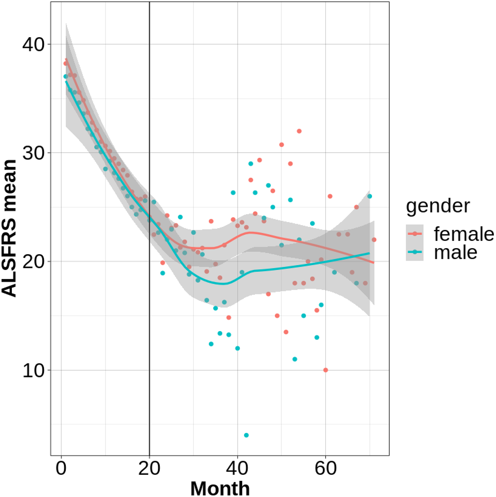
ALS progression distribution with gender.

Figure 5 reflects the ALS progression distribution with a) race, b) respiratory, c) Dyspnea, d) Salivation conditions. Figure 5(a) to (d) illustrates the progression of ALS, as measured by mean ALSFRS-R scores over time, categorized by race, respiratory function, dyspnea, and salivation. All graphs demonstrate a general decline in functional ability across time, with a vertical line at 20 months potentially marking a significant study point. Figure 5(a) suggests potential early-stage differences in decline rates across racial groups, though long-term trends are similar. Figures 5(b) and (c), and (d) reveal strong correlations between respiratory function, dyspnea, and salivation difficulties, respectively, and the rate of ALSFRS-R score decline, with more severe symptoms associated with faster progression. These visualizations underscore the importance of these clinical factors in understanding ALS heterogeneity and identifying key prognostic indicators.

Figure 5.

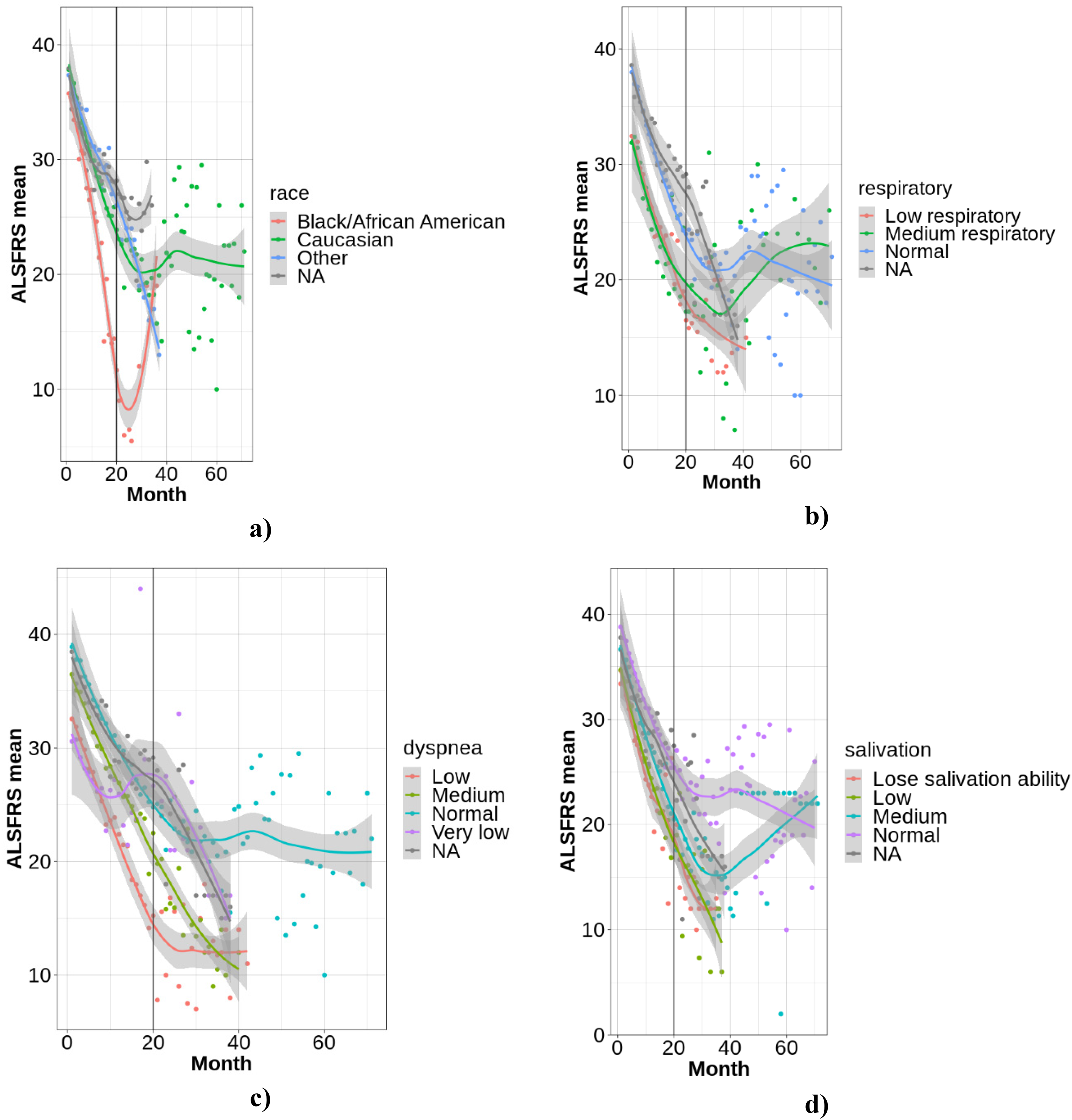
a) Race, b) respiratory, c) dyspnea, d) salivation.

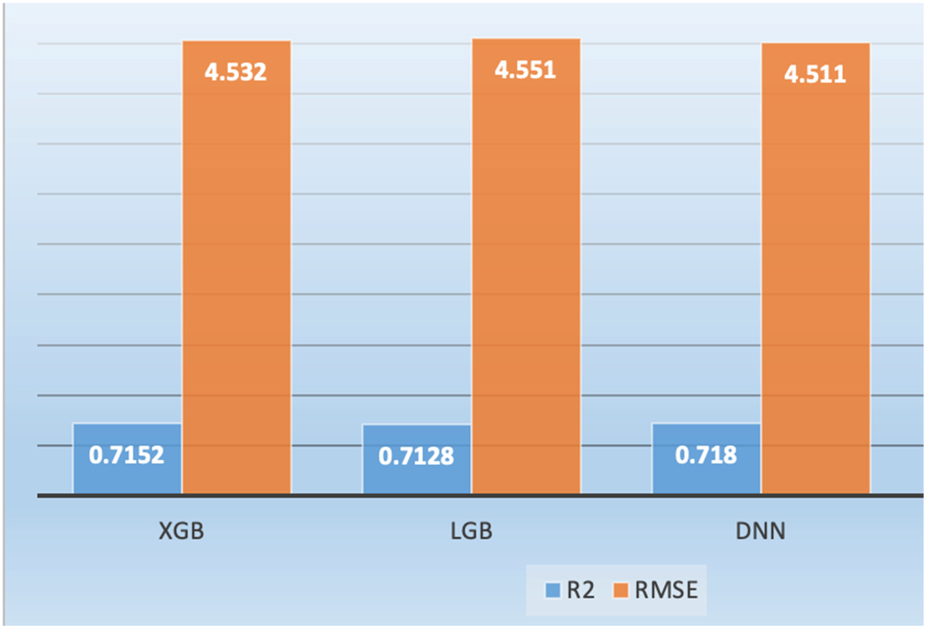
Figure 6 presents the ALS progression for test data with optimized parameters utilizing different machine learning models such as XGB, LGB, and DNN (1D Sequential CNN) model. We also computed the hybrid approach by combining the machine learning models with DNN. We computed the performance based on R-squared, RMSE, slope, intercept, skewness. The greatest R-squared value indicates the better progression prediction while smaller RMSE indicate the better prediction. Based on the default parameters, the DNN model yielded the R-squared (0.718), XGB with R2 (0.7152), LGB with R2 (0.7128). The RMSE yielded by DNN was 4.511, XGB with RMSE (4.532) and LGB with RMSE (4.551). The ensemble methods (XGB, LGB, DNN) by combining the strengths of all three models further improved the ALS progression by yielding the R2 (0.7188), RMSE (4.5036).

Figure 6.

ALS progression by optimizing the parameters of deep learning and machine learning algorithms.

The bar graph of Figure 6 compares the performance of XGB, LGB, and DNN in predicting ALS progression, using R-squared (R2) and RMSE as evaluation metrics. All three models demonstrate comparable performance, with R2 values exceeding 0.71, indicating a reasonable fit to the data, and RMSE values around 4.5, suggesting similar prediction error magnitudes. Notably, the DNN exhibits a slightly higher R2, suggesting it explains more variance in the data, while XGB shows a marginally lower RMSE, indicating slightly more accurate predictions on average. These results suggest that all models are viable for ALS progression prediction, with the choice between DNN and XGB potentially dependent on the specific research priorities.

Figure 7 reflects the ALS progression utilizing the deep learning 1dCNN and comparing the results with machine learning XGB and LGB with default parameters. The DNN yielded the R2 (0.716), XGB with R2 (0.709), and LGB (0.713). The RMSE to predict the ALS progression based on default parameters was 4.56, XGB with RMSE (4.62), LGB with RMSE (4.56).

Figure 7.

ALS progression with default parameters of deep learning and machine learning algorithms.

The bar graph of Figure 7 illustrates the predictive performance of XGBoost (XGB), LightGBM (LGB), and a Deep Neural Network (DNN) for ALS progression using default parameters, as evaluated by R-squared (R2) and Root Mean Squared Error (RMSE). The DNN consistently outperforms both XGB and LGB, exhibiting the highest R2 value and the lowest RMSE, indicating superior variance explanation and prediction accuracy. While all models demonstrate reasonable performance with default settings, the DNN's edge suggests it is inherently better suited to the ALS progression data's characteristics. This comparison provides a baseline for evaluating the impact of hyperparameter optimization and highlights the DNN's potential as a strong candidate for predicting ALS progression without extensive tuning.

Figure 8 reflects the ALS progression of one year utilizing deep learning and comparing results with machine learning. The R2 was yielded utilizing DNN (0.755), XGB (0.749) and LGB (0.754). The RMSE yielded utilizing DNN (4.112), XGB (4.163) and LGB (4.123).

Figure 8.

ALS progression by optimizing the parameters of deep learning and machine learning algorithms for one year.

The bar graph of Figure 8 compares the performance of XGBoost (XGB), LightGBM (LGB), and a Deep Neural Network (DNN) in predicting ALS progression over one year, after optimizing their parameters, using R-squared (R2) and Root Mean Squared Error (RMSE) metrics. All models demonstrate improved performance compared to their default parameter settings, highlighting the effectiveness of hyperparameter tuning. The DNN exhibits the highest R2 and lowest RMSE, indicating slightly superior predictive accuracy, though the differences between the models are marginal. This suggests that while all three models are viable for predicting one-year ALS progression, the DNN offers a slight advantage in both capturing data variance and minimizing prediction error, making it a potentially preferred choice depending on specific research priorities.

Figure 9 shows a comparison of deep learning (DL) and machine learning (ML) algorithms for ALS progression prediction over a period of 40 months. The compared algorithms were convolutional neural networks (CNN), eXtreme Gradient Boosting (XGBoost), and light gradient boosting machine (LGB). The three algorithms showed encouraging predictive ability, with different strengths. CNN obtained the maximum R-squared (0.716) and the minimum after the lowest Root Mean Squared Error (RMSE) (4.565), indicative of its capabilities to model sophisticated data relationships as well as output reliable predictions. XGBoost attained a slighter lower R-squared (0.709) and somewhat greater RMSE (4.625), evidence of its high potential in understanding feature relationships but, in this particular instance, somewhat less successfully than CNN. LGB had an R-squared of 0.713 and an RMSE of 4.595, closely matching CNN and demonstrating its ability to process complex data and derive useful predictive features.

Figure 9.

ALS progression by optimizing the parameters of deep learning and machine learning algorithms for 40 months.

Figure 9, a bar graph, illustrates the predictive performance of XGBoost (XGB), LightGBM (LGB), and a Deep Neural Network (DNN) for ALS progression, using their default parameters, as quantified by R-squared (R²) and Root Mean Squared Error (RMSE). The DNN demonstrably exhibits the highest R² and lowest RMSE, indicating superior variance explanation and prediction accuracy compared to XGB and LGB. Although all three models demonstrate acceptable performance with default settings, the DNN's consistent advantage suggests it is inherently better aligned with the characteristics of the ALS progression data without requiring explicit tuning. This graph serves as a baseline for assessing the impact of subsequent hyperparameter optimization and underscores the DNN's potential as a robust predictor of ALS progression, even without extensive parameter adjustments.

Figure 10 presents a comparative analysis of the predictive performance of XGBoost (XGB), LightGBM (LGB), a deep neural network (DNN), and an ensemble model for ALS progression over a 40-month period, subsequent to hyperparameter optimization. All four models exhibited comparable predictive capabilities, with only marginal variations in performance. Notably, the ensemble model achieves the highest R-squared (R2) value and the lowest root mean squared error (RMSE), indicating a slight but consistent improvement in both variance explanation and prediction accuracy compared to the individual models. This finding underscores the potential benefits of ensemble methods in enhancing predictive performance by combining the strengths of multiple algorithms. While the DNN performs closely to the ensemble, the ensemble's marginal advantage suggests that it effectively leverages the diverse predictive patterns captured by the individual models, highlighting its potential for more robust and accurate ALS progression prediction.

Figure 10.

ALS progression with hyperparameter optimization for 40 months.

Figure 11 presents a comprehensive scatter plot analysis comparing the observed and predicted ALS progression values across four distinct models, accompanied by residual plots to assess error distribution. The left column illustrates the relationship between observed and predicted values, where models 2, 3, and 4 demonstrate superior performance compared to model 1, evidenced by higher R-squared values and lower RMSE. Notably, model 4, likely an ensemble model, exhibits the best fit with the highest R-squared and lowest RMSE, indicating the most accurate predictions. The right column displays residual plots, revealing a somewhat random scatter around zero for all models, though a slight tendency towards negative residuals at higher observed values suggests potential heteroscedasticity. Overall, the figure highlights the effectiveness of models 2, 3, and 4 in predicting ALS progression, with model 4 demonstrating the most robust performance, while also indicating areas for potential model refinement to address heteroscedasticity.

Figure 11.

Scattered graph for ALS progression observed vs predicted left) predicted, right) observed on test data.

Both machine learning and deep learning algorithms demonstrated favorable results in predicting ALS progression over a 40-month period. Convolutional neural networks (CNNs) achieved the highest R-squared (0.716) and the second-lowest root mean squared error (RMSE) (4.565), indicating its efficacy in capturing complex data relationships. eXtreme Gradient Boosting (XGBoost) and light gradient boosting machine (LGB) yielded R-squared values of 0.709 and 0.713, respectively, with marginally higher RMSE values, demonstrating their ability to learn feature relationships and process complex data. Scatter plots, as depicted in Figure 11, comparing observed and predicted ALS progression, further illustrate the strengths and limitations of each model. XGBoost and LGB exhibited tight clustering of points around the diagonal, signifying accurate predictions for the majority of data points. The DNN scatter plot displayed a wider distribution, suggesting increased prediction errors. Of note, the ensemble model had the closest clustering, verifying its high predictive precision. Quantitative measurements like R-squared and RMSE also verify the findings. R-squared values for XGBoost, LGB, and the ensemble model were above 0.7, meaning the correlations between the predicted and actual values are very strong. Also, the lowest values for RMSE were reported by XGBoost and LGB, affirming their accuracy in forecasting ALS development. The ensemble model was superior to single models in R-squared and RMSE, showing its applicability for improved prediction. The strengths of the study are a thorough comparison of models, hyperparameter tuning, visualization and quantitative analysis, and the illustration of the superiority of an ensemble model. Future studies can look into combining other sources of data, creating explainable models, and applying findings to practice. Through further insights into ALS progression and more accurate prediction methods, we can enable better management of the disease and care for the patient.

The boxplots for residuals (discrepancies between predicted and actual ALS progress value) distribution across two models, XGB and LGB, for month-grouped months can be found in Figure 12(a) and (b). On the y-axis are the residues and on the x-axis, there are labels marking the months. For XGB as illustrated in Figure 12(a), the residuals exhibit a fairly stable median close to zero throughout most months, which means unbiased predictions on average. There is, however, higher variability, especially in months 6 and 8, indicating possible variations in prediction accuracy. Similarly, in the case of LGB Figure 12(b), residuals are roughly zero-centered, yet more varied from months 6 to 9, with the range and outliers clearly rising. This implies that although both models are generally unbiased, the consistency of predictions from these models across different months is not even, with LGB being more seriously unstable for later months.

Figure 12.

Boxplot for ALS progression observed vs predicted a) XGB, b) LGB, c) DNN, d) Ensemble on test data.

Figure 12(c) and (d) show boxplots of a comparison of residual distributions between a deep neural network (DNN) and an ensemble model for prediction of ALS progression, stratified by month. Both models show median residuals close to zero in most months, suggesting unbiased prediction on average. Nevertheless, the ensemble model displays more consistency in terms of thinner boxplots with fewer outliers compared to the DNN, hinting at smaller variability and increased reliability in the predictions. Interestingly, both models exhibit higher residual variability in months 6, 8, and 9, suggesting possible difficulties in predicting ALS progression during these particular months. This implies that although both models are generally good, the ensemble model provides slightly more stable and accurate predictions, and it highlights the advantages of model combination and the need for further research into the higher prediction variability noted during these specific months. Figure 12 conveys important information on the performance of different machine and deep learning models in the first ten months of ALS progression, represented using boxplots.

These plots describe how effectively every model reflects inherent early-stage ALS variability. There was dispersion of predicted values from all models, with months 5–8 showing exceptionally high variability, corresponding to a peak predictive uncertainty phase. Interquartile range (IQR), an indication of prediction clumping, showed considerable variation across models. The widest IQR was seen for XGBoost, implying this model could possibly fail to repeatedly identify early changes in progression as subtle. LightGBM (LGB) showed better consistency with a tighter IQR, whereas the DNN underestimated progression with its low median and tight IQR. In contrast, the ensemble model had the tightest IQR and median closest to observed values, affirming its better accuracy in early-stage prediction. Error distribution analysis also supported these observations, with the DNN and ensemble model showing lower error rates. This discussion highlights the need for stage-specific model assessment, especially in initial ALS, where early changes require high sensitivity. Upcoming studies must aim to detect influential features, create hybrid models for various disease stages, and improve explainable AI to increase clinician confidence. Boxplots and error analysis are crucial for fine-tuning these models to ultimately enable enhanced early diagnosis, monitoring, and personalized treatment strategies for ALS patients.

Table 1 presents the performance of four optimized machine learning algorithms in classifying ALS onset type, with XGBoost demonstrating exceptional accuracy. XGBoost achieved perfect sensitivity (100%), correctly identifying all bulbar onset cases, and high specificity (97.44%), accurately classifying nearly all limb onset cases. Its positive predictive value (90.91%) and negative predictive value (100%) further underscore its reliability. Overall, XGBoost achieved an accuracy of 97.96%, with an F1-score of 95.24% and an MCC of 94.12%, indicating a highly effective and balanced performance. In contrast, the Decision Tree model showed moderate sensitivity (47.37%) and good specificity (93.33%), but its overall accuracy was only 75.51%, with an F1-score of 28.42% and an MCC of 47.53%, indicating limited effectiveness in bulbar onset classification. The KNN model performed the poorest, with low sensitivity (33.33%) and moderate specificity (88%), resulting in an accuracy of 61.22%, an F1-score of 15.24%, and an MCC of 25.56%, highlighting its unsuitability for this classification task. Similarly, the SVM Quadratic model showed moderate sensitivity (44.44%) and good specificity (90.32%), with an accuracy of 73.47%, an F1-score of 24.52%, and an MCC of 40.17%, indicating challenges in accurately classifying bulbar onset cases. Thus, XGBoost stands out as the most reliable and accurate classifier for distinguishing between bulbar and limb onset ALS in this dataset.

Table 1.

ALS bulbar vs limb detection and classification using optimized machine learning algorithms.

Classifier	Sens.	Spec.	PPV	NPV	Accuracy	F1-Score	MCC
XGBoost	1.0000	0.9744	0.9091	1.0000	0.9796	0.9524	0.9412
DT	0.4737	0.9333	0.8182	0.7368	0.7551	0.2842	0.4753
KNN	0.3333	0.8800	0.7273	0.5789	0.6122	0.1524	0.25561
SVM Q	0.4444	0.9032	0.7273	0.7368	0.7347	0.2452	0.4017

Table 2 summarizes the classification report for an optimized XGBoost model's performance in distinguishing between limb (class 0) and bulbar (class 1) onset ALS. For limb onset, the model obtained a precision of 100% as all limb onset predictions were correct, and a recall of 91% as it identified 91% of true limb onset cases. This yielded an F1-score of 95%, indicating a strong balance between precision and recall. For bulbar onset, the model showed a high precision of 97%, indicating that 97% of the bulbar onset cases predicted were correct, and a perfect recall of 100%, identifying all true bulbar onset cases, with an F1-score of 99%. The model overall achieved an accuracy of 98%, classifying 98% of all cases correctly. The macro-average F1-score was 97%, and the weighted-average F1-score was 98%, which further emphasizes the model's superior and well-balanced performance for both classes. This report emphasizes the high reliability and accuracy of the optimized XGBoost model in predicting ALS onset type classification.

Table 2.

ALS bulbar vs limb detection and classification report using optimized XGBoost.

Class	Precision	Recall	F1-Score	Support
0	1.00	0.91	0.95	11
1	0.97	1.00	0.99	38
Accuracy			0.98	49
Macro Avg	0.99	0.95	0.97	49
Weighted Avg	0.98	0.98	0.98	49

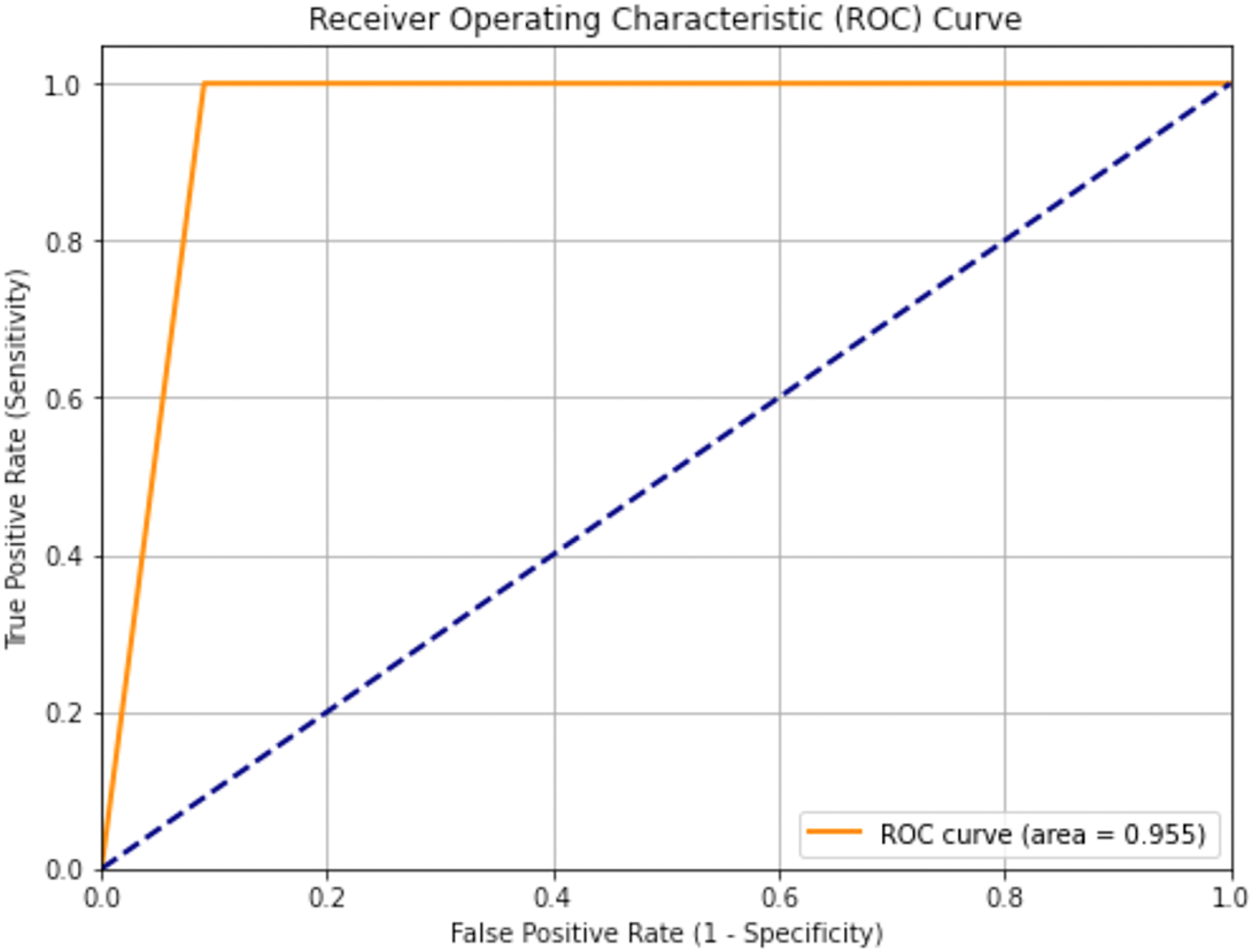
Figure 13 shows the receiver operating characteristic (ROC) curve of an optimized XGBoost model trained to predict ALS onset type, with a high area under the curve (AUC) of 0.955. This AUC value indicates outstanding discriminatory power, reflecting the model's strong capacity to distinguish between bulbar and limb onset ALS. The ROC curve's placement well above the diagonal line, which is a random classifier, and its steep rise towards the top-left corner, further confirm the model's high sensitivity with a low false positive rate. These findings indicate that the optimized XGBoost model is extremely effective and may be a useful tool in clinical practice for the accurate classification of ALS onset type.

Figure 13.

AUC to classify bulbar vs limb using optimized XGBoost.

Figure 14 displays the ALS Functional Rating Scale (ALSFRS) class median distribution, with a clear bimodal pattern defined by two peaks centered on values of 0 and 1. The bimodality indicates that there are two discrete clusters in the dataset, which may be indicative of different stages of ALS progression or different patient subgroups. The red dashed line, which symbolizes the mean, lies in between these two peaks, demonstrating the effect that both clusters have on the mean value. From the density plot and histogram together, it can be seen that these two clusters are the most common within the data, so there is an apparent categorization or transformation that has been carried out on the original ALSFRS data.

Figure 14.

ALSFRS class median distribution.

Figure 15 presents the distribution of the ALSFRS class median, showing a unimodal distribution with slight right skewing, which means that although most of the values are bunched around a point, there are afew larger values stretching the tail of the distribution. The mean value, marked at 24.67, provides a measure of central tendency, suggesting the average ALSFRS class median in the dataset. The spread of the histogram and the superimposed kernel density estimation curve indicate variability in the data, reflecting a range of disease progression among the patient population. This distribution, while approximately normal, highlights the presence of some individuals with higher ALSFRS class median values, contributing to the observed skew.

Figure 15.

Distribution of ALSFRS class median.

Figure 16 displays the distribution of the WASH7P feature, revealing a unimodal shape with a slight right skew, indicating a central tendency around the 50–60 range while suggesting the presence of some higher values extending the distribution's tail. The density plot and histogram together illustrate the frequency and probability of WASH7P values, showing a relatively spread-out distribution that reflects variability in the data. This visualization provides insights into the feature's characteristics, highlighting its central tendency and potential for outliers, which can inform data preprocessing and feature importance assessments.

Figure 16.

Distribution of feature WASH7P.

Figure 17 presents the feature importance of the top eight ranked features as determined by an XGBoost model, illustrating their relative influence on the model's predictions. The horizontal bar chart clearly ranks the features, with ZBTB2P1 emerging as the most significant, followed by RNF181, and descending in importance to WASH9P, which is the least influential among the top eight. The length of each bar directly corresponds to the feature's importance score, providing a visual representation of their relative contributions. This visualization serves as a valuable tool for understanding which features the XGBoost model prioritizes, offering insights for feature selection, domain-specific analysis, and model interpretation.

Figure 17.

Feature importance of top 8 ranked features using XGBoost.

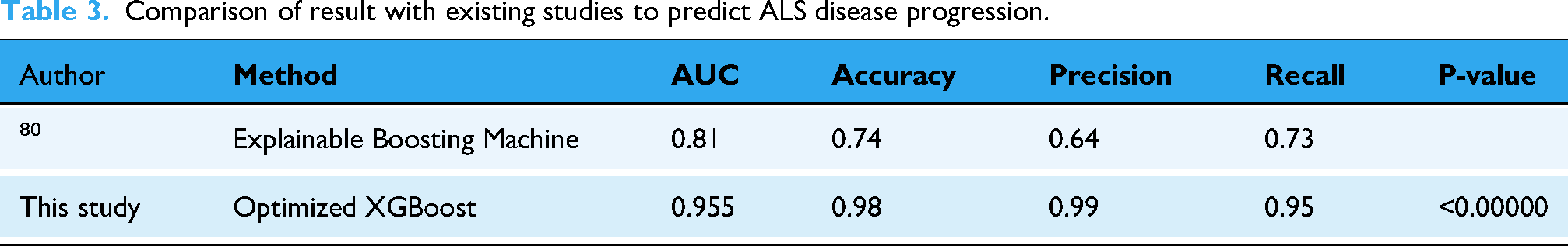
A comparative analysis of ALS disease progression prediction models as reflected in Table 3 reveals a significant performance boost achieved by the current study's Optimized XGBoost method. Compared to the explainable boosting machine used in a previous study, the XGBoost model demonstrated substantial improvements across all key metrics. Notably, the AUC increased from 0.81 to 0.955, accuracy jumped from 0.74 to 0.98, and precision soared from 0.64 to 0.99. This superior performance, reflected in high recall and F1-scores, underscores the effectiveness of the optimized XGBoost approach for this specific application. These results suggest that the model holds significant clinical potential for accurately predicting ALS progression, which could greatly aid in patient management and research efforts. The paired t-test yielded the highly significant results to distinguish the Bulber from Limb subjects.

Table 3.

Comparison of result with existing studies to predict ALS disease progression.

Author	Method	AUC	Accuracy	Precision	Recall	P-value
80	Explainable Boosting Machine	0.81	0.74	0.64	0.73
This study	Optimized XGBoost	0.955	0.98	0.99	0.95	<0.00000

The XGBoost, LightGBM and 1D CNN are chosen because of the best balance of performance, interpretability, and compatibility with the available dataset and computational resources.

The proposed model offers several key findings and outcomes that enhance the prediction and monitoring of ALS disease progression, facilitating improved treatment strategies:

Early Risk Stratification: The model enables the identification of patients at elevated risk for rapid disease progression, empowering neurologists to implement timely interventions. For example, patients predicted to experience a substantial decline in ALS Functional Rating Scale-Revised (ALSFRS-R) scores within a defined period can be prioritized for more frequent follow-up appointments and intensified symptom management.

Personalized Treatment Planning: By predicting individual patient responses to various therapies, the model aids in tailoring personalized treatment plans. For instance, if the model predicts a high probability of a patient benefiting from a specific experimental drug, neurologists can consider their enrollment in relevant clinical trials.

Enhanced Prognostic Communication: The model provides more precise and objective prognostic information, which is essential for patients and their families to make informed decisions regarding care and end-of-life planning.

Diagnostic Support: The model can serve as a supplementary tool to assist in identifying patients who may have ALS, particularly in the early stages of the disease.

Streamlined Disease Monitoring: The model provides objective, quantitative measures of disease progression, reducing reliance on subjective assessments.

Improved Clinical Decision-Making: By delivering evidence-based predictions, the model supports neurologists in making informed decisions about patient management.

The outputs of our proposed model can be integrated into various devices to enhance the efficacy of healthcare systems for individuals with ALS, including:

Home-Based Forced Vital Capacity (FVC) Monitoring Devices: Integration with home-based FVC devices enables real-time monitoring of respiratory function. For instance, if the model predicts a rapid decline in FVC, an alert can be transmitted to the patient's neurologist, prompting immediate intervention.

ALS Functional Rating Scale-Revised (ALSFRS-R) Tracking Applications: Integration with mobile applications tracking ALSFRS-R scores provides a comprehensive overview of disease progression.

Wearable Sensor Data Collection Platforms: Integration with wearable sensor data, monitoring activity levels, sleep patterns, and other physiological parameters, offers a holistic view of patient health.

Electronic Health Record (EHR) Systems: Direct integration into EHR systems facilitates real-time risk assessments during patient encounters.

To strengthen the connection to ALS pathophysiology, the manuscript should integrate a more detailed discussion of how identified features relate to the disease's underlying biological mechanisms. For instance, the prominence of FVC decline in the model aligns with the established understanding of respiratory muscle weakness as a critical factor in ALS progression, reflecting progressive motor neuron degeneration.

Likewise, the significance of certain lab values may reflect systemic inflammation or metabolic derangements leading to neuronal injury. Feature importance analyses need to be interpreted in the context of existing neurodegenerative knowledge, for example, the propagation of pathological protein aggregates or the involvement of glutamate excitotoxicity, with reference to pertinent literature. Recognizing the heterogeneity of ALS and elaborating on how the model could potentially capture different disease subtypes or patterns of progression would add further biological plausibility to the study. Although the model has excellent predictive performance, it is important to note its limitations in completely representing the complexity of ALS pathophysiology and to propose future directions for research that include multi-omics data or longitudinal biomarker studies to better understand the disease mechanisms. To counteract the problem of ‘black-box’ models within clinical environments, our research incorporated a number of interpretability approaches to build clinician trust and enable real-world application.

We employed SHAP value analysis in offering personalized explanations to model predictions to illustrate the effect of specific features, for instance, Forced Vital Capacity (FVC) worsening and elevated lab values, toward each patient's risk determination. This was not only helping elucidate how the model had decided but was also consistent with published clinical practice and knowledge so that clinicians were better able to justify and act upon the predictions. In addition, world feature importance estimation, based on the XGBoost model, identified the relative importance of clinical factors, such as ALSFRS-R sub-scores and time since diagnosis, providing practitioners with useful guidelines for prioritizing patient surveillance and intervention strategies. By including these interpretability tools, we endeavored to make the gap between sophisticated predictive models and their pragmatic clinical application narrow, making sure that our conclusions are transparent as well as actionable.

Conclusions

The speedily growing presence of biomedical data is revolutionizing healthcare, creating tremendous potential for the creation of predictive models via data-driven techniques and machine learning. The paper responds to domain-specific and technological issues in developing a model to predict ALS progression. ALS is a progressive neurodegenerative disorder with poor therapeutic prospects and needs precise predictive models urgently. Survival of the patients, which normally ranges between three and five years, is governed by genetic, demographic, and phenotypic factors, thereby reflecting the intricacy of the disease. Pharmaceutical development is hampered by a lack of definitive disease progression biomarkers, causing problems in clinical trials, such as patient enrollment delay and diverse patient populations. Additionally, an appreciable diagnostic delay, amounting to roughly one year between the onset of symptoms and diagnosis, impedes the administration of potentially useful treatments.

Utilizing the PRO-ACT dataset, this study evaluated machine learning and deep learning models for ALS progression prediction and onset type classification. Initial evaluation with default parameters showed the deep learning model outperformed XGBoost and LightGBM, achieving an RMSE of 4.565 and R2 of 0.716. Hyperparameter optimization further improved the deep learning model's accuracy (RMSE: 4.511, R2: 0.718) and yielded slight gains in XGBoost and LightGBM. Optimized XGBoost achieved exceptional classification performance for bulbar vs. limb onset ALS, with 100% sensitivity, 97.44% specificity, 97.96% accuracy, 95.96% F1-score, 94.12% MCC, and 0.9550 AUC. Feature importance analysis identified ZBTB2P1 as the most influential feature. These results demonstrate the potential of optimized XGBoost and deep learning for accurate ALS prediction and classification, enabling improved patient management and potentially reducing mortality.

Limitations and future directions

This study, while demonstrating promising results in ALS progression prediction and classification using machine learning and deep learning, acknowledges limitations related to the sensitivity and specificity of current assessment measures, as well as challenges posed by late-stage clinical trial recruitment and disease heterogeneity. Future research should focus on developing explainable AI models to enhance clinical trust, incorporating diverse data sources like imaging and genetics for improved accuracy, and exploring hybrid models tailored to specific disease stages.

In addition, their application to plan more effective clinical trials with fewer sample sizes and creating AI-based software for automated monitoring and diagnosis of disease are critical milestones. Continued optimization of the models will eventually lead to personalized treatment protocols and improved patient outcomes.

This research acknowledges that although data augmentation and imputation are vital for dealing with missing datasets, they have limitations that need to be explored. Imputation techniques risk bias and loss of information, making it necessary to come up with distribution-preserving methods and measures of uncertainty quantification, especially in longitudinal research where temporal dependencies are hard to maintain. Likewise, data augmentation can impart artifacts and overfitting, necessitating the creation of realistic synthetic samples and adaptive methods, with focus on clinical appropriateness and stringent assessment. Research in the future will need to give high importance to hybrid methodologies, deep learning methods, and uncertainty quantification with a view to reducing bias and increasing the reliability of these data preprocessing methods.