Sage Journals: Discover world-class research

Abstract

French

Background:

Safety issues are detected in about one third of prescription drugs in the years following regulatory agency approval. Older adults, especially those with chronic kidney disease, are at particular risk of adverse reactions to prescription drugs. This protocol describes a new approach that may identify credible drug-safety signals more efficiently using administrative health care data.

Objective:

To use high-throughput computing and automation to conduct 700+ drug-safety cohort studies in older adults in Ontario, Canada. Each study will compare 74 acute (30-day) outcomes in patients who start a new prescription drug (new users) to a group of nonusers with similar baseline health characteristics. Risks will be assessed within strata of baseline kidney function.

Design and setting:

The studies will be population-based, new-user cohort studies conducted using linked administrative health care databases in Ontario, Canada (January 1, 2008, to March 1, 2020). The source population for these studies will be residents of Ontario aged 66 years or older who filled at least one outpatient prescription through the Ontario Drug Benefit (ODB) program during the study period (all residents have universal health care, and those aged 65+ have universal prescription drug coverage through the ODB).

Patients:

We identified 3.2 million older adults in the source population during the study period and built 700+ initial medication cohorts, each containing mutually exclusive groups of new users and nonusers. Nonusers were randomly assigned cohort entry dates that followed the same distribution of prescription start dates as new users. Eligibility criteria included a baseline estimated glomerular filtration rate (eGFR) measurement within 12 months before the cohort entry date (median time was 71 days before cohort entry in the new user group), no prior receipt of maintenance dialysis or a kidney transplant, and no prior prescriptions for drugs in the same subclass as the study drug. New users and nonusers will be balanced on ~400 baseline health characteristics using inverse probability of treatment weighting on propensity scores within 3 strata of baseline eGFR: ≥60, 45 to <60, <45 mL/min per 1.73 m².

Outcomes:

We will compare new user and nonuser groups on 74 clinically relevant outcomes (17 composites and 57 individual outcomes) in the 30 days after cohort entry. We used a prespecified approach to identify these 74 outcomes.

Statistical analysis plan:

In each cohort, we will obtain eGFR-stratum-specific weighted risk ratios and risk differences using modified Poisson regression and binomial regression, respectively. Additive and multiplicative interaction by eGFR category will be examined. Drug-outcome associations that meet prespecified criteria (identified signals) will be further examined in additional analyses (including survival, negative-control exposure, and E-value analyses) and visualizations.

Results:

The initial medication cohorts had a median of 6120 new users per cohort (interquartile range: 1469-38 839) and a median of 1 088 301 nonusers (interquartile range: 751 697-1 267 009). Medications with the largest number of new users were amoxicillin trihydrate (n = 1 000 032), cephalexin (n = 571 566), prescription acetaminophen (n = 571 563), and ciprofloxacin (n = 504,374); 19% to 29% of new users in these cohorts had an eGFR <60 mL/min per 1.73 m².

Limitations:

Despite our use of robust techniques to balance baseline indicators and to control for confounding by indication, residual confounding will remain a possibility. Only acute (30-day) outcomes will be examined. Our data sources do not include nonprescription (over-the-counter) drugs or drugs prescribed in hospitals and do not include outpatient prescription drug use in children or adults <65 years.

Conclusion:

This accelerated approach to conducting postmarket drug-safety studies has the potential to more efficiently detect drug-safety signals in a vulnerable population. The results of this protocol may ultimately help improve medication safety.

Keywords

adverse drug events automation chronic kidney disease drug safety high-throughput computing machine learning medication drug pharmaco-epidemiology pharmaco-informatics pharmacovigilance postmarket drug surveillance real-world data

Introduction

The safety profile of a prescription drug is not fully known at the time it is released to the market. The process used by regulatory agencies to approve drugs is primarily based on a review of data from clinical trials that follow a limited number of patients under highly controlled conditions. After a drug has been approved, regulatory agencies such as the U.S. Food and Drug Administration and Health Canada subsequently rely on further evaluation to identify unintended pharmacologic effects of prescription drugs. Safety issues are detected in about one third of drugs in the years following approval.¹

Older adults are at particular risk—about 1 in 6 hospitalizations among older adults are for adverse drug events.² Older adults with chronic kidney disease (CKD) are typically underrepresented in initial drug trials; thus, the efficacy and safety of approved drugs are often unclear in these patients. Recommended dosages may not generalize to older patients due to age-related changes in the body’s ability to absorb, metabolize, and excrete drugs. Kidney function declines with age, and about one third of adults older than 65 have an estimated glomerular filtration rate (eGFR) below 60 mL/min per 1.73 m² (a diagnostic criterion for CKD). Low kidney function prolongs the half-life of drugs and metabolites that are cleared by the kidneys; to avoid toxicity, these medications often need to be dose-reduced or avoided entirely in patients with CKD.

Over the past decades, pharmaco-epidemiology has answered a wide range of study questions using various data sources and analytic methodologies. Several population-based studies have quantified the risk of unintended harms of medications and informed safer prescribing in vulnerable populations, including those excluded from trials, such as pregnant women, multimorbid patients, and older adults. Unfortunately, this process can be slow and inefficient. Unanticipated harmful drug effects usually first come to light in case reports and from the analysis of spontaneous reporting databases. If enough reports accumulate, large pharmaco-epidemiologic studies may be conducted. However, each of these pharmaco-epidemiologic studies usually examines only 1 or 2 drugs and only a few outcomes. With this approach, many harmful effects are missed, and small knowledge gains take years to achieve.

In this protocol, we describe our plan to detect drug-safety signals more efficiently in older adults with CKD in routine care. Using high-throughput computing and automation, we will conduct 700+ population-based, new-user, drug-safety studies using 12 years of data from Ontario’s administrative health care databases (2008-2020). These databases contain encrypted data on all health care visits, hospitalizations, and laboratory results of Ontario residents—all residents have universal access to hospital care and physician services through a government-funded single-payer system, and Ontarians aged 65 years and older also receive universal outpatient prescription drug coverage.

We describe the methods we used to build these 700+ medication cohorts, each containing new-user and nonuser groups that will be statistically balanced on 400+ baseline health characteristics. We describe the process we used to select and define 74 clinically relevant outcomes and our statistical analysis plan for the main analysis to identify potential drug-safety signals in CKD and minimize the chance of false discoveries. Drug-outcome associations that meet prespecified criteria will be examined further in multiple additional and exploratory analyses, including survival, negative-control exposure, and E-value analyses.

Methods

Study Design, Setting, and Data Sources

Using high-throughput computing and automation, we will conduct 700+ population-based, new-user, drug-safety cohort studies using linked administrative health care databases in Ontario, Canada. The study period will be from January 1, 2008, to March 1, 2020. All study data will be obtained from Ontario’s linked administrative health care databases housed at ICES.³ These databases contain encrypted, person-level data for Ontario residents, all of whom have universal access to hospital care and physician services through a government-funded single-payer system. Residents aged 65 years and older also receive universal prescription outpatient drug coverage, whereas residents of all ages receive universal prescription drug coverage when they are in the emergency department or are admitted to hospitals. Thus, our studies will use outpatient dispensing information of all prescription drugs for residents aged 65 years and older. We have previously used these databases to study adverse drug events and health outcomes.^4-8 Except for data on prescriber specialty (10%-20% missing) and neighborhood income quintile (0.01%-1.72%), these databases are complete for all variables. Emigration from the province, which occurs at a rate of 0.5% per year, is the only reason for the loss to follow-up.⁹ The use of data in this study is authorized under section 45 of Ontario’s Personal Health Information Protection Act, which does not require review by a research ethics board. The datasets will be linked using unique encoded identifiers and analyzed at the ICES.

More details on the databases, study variables, and the codes used to ascertain baseline comorbidities are provided in Supplemental eTable 1. Study conduct and reporting will follow recommended guidelines for observational pharmaco-epidemiology studies that use routinely collected health data.^10-12

In preparation for conducting these studies, we built multiple medication cohorts of new users and nonusers. We will employ a high-throughput computing environment to facilitate the parallel processing of medication cohorts. Our statistical and machine learning operations will be carried out using SAS, R, and Python. In addition, we plan to use the open-source JavaScript library D3 for the development of interactive visualizations. Described below is the process we used to integrate data from different sources (Supplemental eFigure 1), build the cohorts, define clinically relevant outcomes for testing in the main analysis (Supplemental eFigure 2), create eGFR-specific cohorts, and calculate propensity scores (Supplemental eFigure 3). We then describe the statistical analysis plan for the main analysis (Supplemental eFigure 4).

Source Population

The source population for the cohort studies comprised residents of Ontario aged 66 years or older who filled an outpatient prescription through the Ontario Drug Benefit (ODB) program from January 1, 2008, to March 1, 2020. The age restriction was applied to ensure at least 1 year of prior prescription drug coverage in this population. The source population contained 3.2 million patients who filled 1.1 billion prescriptions for 745 distinct oral medications during this time. These prescriptions were prescribed by 106 578 unique physicians. This population was restricted to patients with a valid ICES key number (the common number used to link the same patient across different health care databases; restricted to those with a valid ICES key number in prescription records) and to those who had valid/nonmissing data on date of birth and sex (missing in 0.1%-0.2% of prescription records).

Selection of New Users for the Medication Cohorts

We applied the following exclusion criteria to the set of 1.1 billion prescription records for 3.2 million patients (Supplemental eFigure 5). These criteria were applied on or before the first date a medication was dispensed to a patient—this date is termed the index date and was also the patient’s cohort entry date. Patients who were prescribed multiple distinct medications had multiple index dates. As part of data cleaning, we excluded prescription records for patients who were nonpermanent residents of Ontario, who were aged <66 or >105 years on or before the index date, or who had a date of death on or before the index date. The number of records removed for each exclusion step is shown in Supplemental eFigure 6.

We then excluded prescription records with a day-supply ≥100 because these prescriptions were likely for patients planning to leave the province for more than 3 months. While the ODB program allows a maximum prescription duration of 100 days, patients leaving Ontario for more than 3 months are allowed a greater supply (e.g., many Ontarians leave the province for several months during the winter; termed snowbirding). Given the low use of healthcare services by this group in Ontario from January to March, it is advisable for researchers to take into account the snowbird population and its potential influence on evaluations that assume continuous observation.¹³ These prescriptions were excluded to avoid incomplete follow-up because the follow-up period for outcomes is only 30 days. We also excluded records with a day-supply <3 days.

For each prescription record, we used a 180-day lookback period to determine if the medication had been previously prescribed to the patient or if a nonoral version had been prescribed (codes for nonoral versions are provided in Supplemental eTable 2), or if another medication in the same subclass had been prescribed. If any of these criteria were met, the prescription record was excluded. For example, a prescription record for furosemide would be excluded if the patient had been prescribed another loop diuretic (e.g., bumetanide or ethacrynic acid) in the 180 days up to and including the furosemide index date.

We excluded prescriptions for patients with no outpatient test results for serum creatinine in the year before the index date and in those whose baseline eGFR was >150 mL/min per 1.73 m², as the latter are likely the result of data entry errors. We calculated the patients’ baseline eGFRs using the most recent outpatient serum creatinine measurement recorded in the year before the index date. Most older adults in Ontario have at least one serum creatinine measurement each year, and we have shown that single outpatient measures of creatinine can be used to group patients into clinically relevant stable eGFR strata (≥60, 45 to <60, <45 mL/min per 1.73 m²) with reasonable accuracy.¹⁴ In Ontario, serum creatinine concentrations are assessed using a method calibrated to isotope dilution mass spectroscopy. The eGFR was calculated using the new race-free eGFR equation.¹⁵ Additional information about this equation is provided in Supplemental eTable 3.

To ensure the prescription was a new outpatient prescription, we excluded records for patients who were discharged from a hospital or emergency department 2 days before the index date or on the index date because patients in Ontario who start a prescription during a hospital admission would have their outpatient prescription dispensed on the same day or the day after hospital discharge. Finally, we excluded prescription records for patients who were treated for kidney failure (i.e., if the patient received maintenance dialysis or a kidney transplant; diagnosis codes are in Supplemental eTable 4).

Following these exclusions, there were 2 754 744 patients who filled 32 876 726 prescriptions for 717 unique medications. We then restricted this sample to the first prescription filled, which left 2 754 744 patients (new users) who filled 23 457 350 prescriptions for one of the 717 medications for the first time during the study period. The median number of new users in each medication cohort was 6120 (interquartile range [IQR]: 1469-38 839).

Selection of Nonusers for the Medication Cohorts

We selected a distinct group of nonusers for each medication cohort as follows. For each cohort, we first selected all patients in the source population who were not part of the cohort’s new-user group. We then randomly assigned cohort entry dates to the nonusers based on the distribution of prescription start dates for the cohort’s new users. The data cleaning steps and eGFR calculations were performed as described for new users, and the full set of exclusions is shown in Supplemental eFigure 6. For example, the baclofen cohort contained 120 606 new users, and we randomly assigned cohort entry dates to the remaining patients in the source population (based on the distribution of prescription start dates for the new users of baclofen). After applying the exclusion criteria described in Supplemental eFigure 7, the nonuser group in the baclofen cohort contained 1 326 036 patients. Overall, the median number of nonusers in each medication cohort was 1 088 301 (IQR: 751 697-1 267 009).

In each cohort, the new-user and nonuser groups will be statistically balanced on 400+ baseline characteristics as described below: Analyses to Balance New-user and Nonuser Groups in Each Cohort.

Outcome Selection

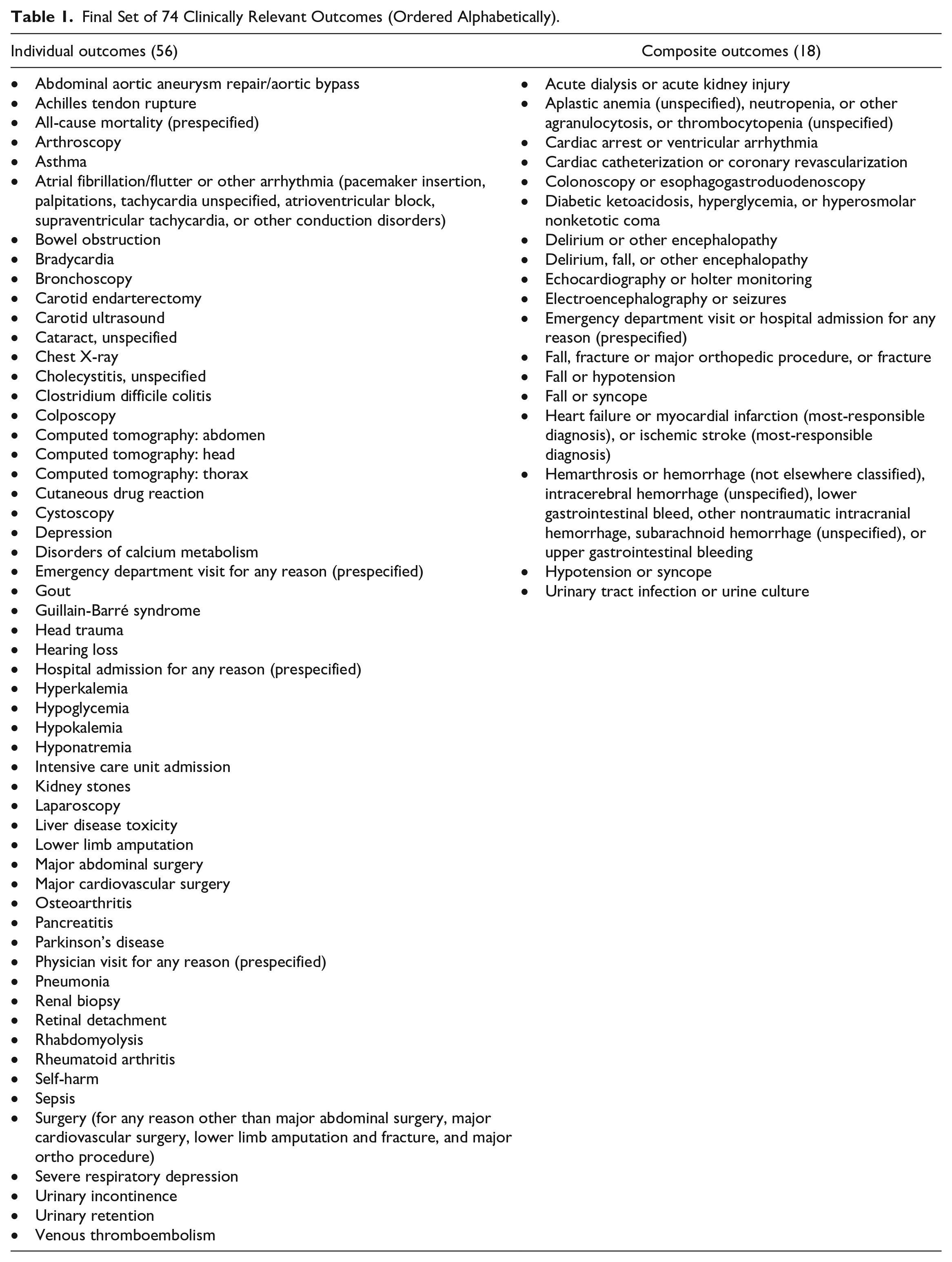
We used a prespecified analytic approach to select 74 clinically relevant outcomes (56 individual and 18 composite outcomes, where 4 of the individual outcomes and 1 of the composite outcomes were prespecified, as shown in Table 1). As described below, we first performed an outcome frequency analysis and identified 89 clinically relevant outcomes that were prevalent in the sample of 2 754 744 new users in the 30-day period after the index date. From this set of 89, we created 17 clinically relevant composite outcomes informed by the results of 3 independent analyses. The remaining 52 outcomes were retained as individual outcomes, and we also prespecified the following 5 outcomes: all-cause mortality, ≥1 hospital admission for any reason, ≥1 emergency department visit for any reason, ≥1 emergency department visit or hospital admission for any reason, and ≥1 physician visit for any reason. We chose a 30-day follow-up period to focus on acute events and to avoid changes in the use of newly prescribed long-term medications that can occur with longer periods of follow-up.

Table 1.

Final Set of 74 Clinically Relevant Outcomes (Ordered Alphabetically).

Individual outcomes (56)

Composite outcomes (18)

• Abdominal aortic aneurysm repair/aortic bypass
• Achilles tendon rupture
• All-cause mortality (prespecified)
• Arthroscopy
• Asthma
• Atrial fibrillation/flutter or other arrhythmia (pacemaker insertion, palpitations, tachycardia unspecified, atrioventricular block, supraventricular tachycardia, or other conduction disorders)
• Bowel obstruction
• Bradycardia
• Bronchoscopy
• Carotid endarterectomy
• Carotid ultrasound
• Cataract, unspecified
• Chest X-ray
• Cholecystitis, unspecified
• Clostridium difficile colitis
• Colposcopy
• Computed tomography: abdomen
• Computed tomography: head
• Computed tomography: thorax
• Cutaneous drug reaction
• Cystoscopy
• Depression
• Disorders of calcium metabolism
• Emergency department visit for any reason (prespecified)
• Gout
• Guillain-Barré syndrome
• Head trauma
• Hearing loss
• Hospital admission for any reason (prespecified)
• Hyperkalemia
• Hypoglycemia
• Hypokalemia
• Hyponatremia
• Intensive care unit admission
• Kidney stones
• Laparoscopy
• Liver disease toxicity
• Lower limb amputation
• Major abdominal surgery
• Major cardiovascular surgery
• Osteoarthritis
• Pancreatitis
• Parkinson’s disease
• Physician visit for any reason (prespecified)
• Pneumonia
• Renal biopsy
• Retinal detachment
• Rhabdomyolysis
• Rheumatoid arthritis
• Self-harm
• Sepsis
• Surgery (for any reason other than major abdominal surgery, major cardiovascular surgery, lower limb amputation and fracture, and major ortho procedure)
• Severe respiratory depression
• Urinary incontinence
• Urinary retention
• Venous thromboembolism

• Acute dialysis or acute kidney injury
• Aplastic anemia (unspecified), neutropenia, or other agranulocytosis, or thrombocytopenia (unspecified)
• Cardiac arrest or ventricular arrhythmia
• Cardiac catheterization or coronary revascularization
• Colonoscopy or esophagogastroduodenoscopy
• Diabetic ketoacidosis, hyperglycemia, or hyperosmolar nonketotic coma
• Delirium or other encephalopathy
• Delirium, fall, or other encephalopathy
• Echocardiography or holter monitoring
• Electroencephalography or seizures
• Emergency department visit or hospital admission for any reason (prespecified)
• Fall, fracture or major orthopedic procedure, or fracture
• Fall or hypotension
• Fall or syncope
• Heart failure or myocardial infarction (most-responsible diagnosis), or ischemic stroke (most-responsible diagnosis)
• Hemarthrosis or hemorrhage (not elsewhere classified), intracerebral hemorrhage (unspecified), lower gastrointestinal bleed, other nontraumatic intracranial hemorrhage, subarachnoid hemorrhage (unspecified), or upper gastrointestinal bleeding
• Hypotension or syncope
• Urinary tract infection or urine culture

Outcome frequency analysis

This analysis was done in a sample of 2 754 744 new users. For each of the 717 study medications, we examined the frequency of 4 types of administrative health care codes recorded in new users within 30 days after the drug dispense date (International Classification of Diseases–10th Revision [ICD-10] codes, Canadian Classification of Health Interventions [CCI] codes, Ontario Health Insurance Plan (OHIP) diagnosis codes, and OHIP fee codes [described in Table 2]). For each medication, we computed the number of unique codes recorded in new users and the number of new users in whom each code was recorded. Then in the sample of all new users, we computed the total number of unique codes recorded and the total number of new users in whom each code was recorded.

Table 2.

Types of Administrative Health Care Codes Used to Define Outcomes in this Study.^16-19

Code type	Description	Database
ICD-10	Classifies diseases, injuries, symptoms, poisoning, complaints, and causes of death during hospital visits (most-responsible diagnosis),^a emergency department visits, and other health care encounters	CIHI-DAD, NACRS,
CCI	Classifies therapeutic and diagnostic interventions and other health care interventions in ambulatory care (outpatient clinics, emergency room visits, and hospital-based surgery).	CIHI-DAD, NACRS
OHIP diagnosis	Diagnosis codes used in reimbursement claims for services provided by physicians and community-based labs. The codes are used to classify diseases, injuries, symptoms, poisonings, and other reasons for patient encounters.	OHIP
OHIP fee code	Fee codes used in reimbursement claims for services provided by physicians and community-based labs. Each record represents a single service, identified by the fee code, although that service may be performed several times. For example, if a child has a myringotomy and an adenoidectomy during the surgery, this will generate 2 records, 1 for the myringotomy and 1 for the adenoidectomy.	OHIP

Note. ICD-10 = International Classification of Diseases–10th Revision; CIHI = Canadian Institute of Health Information; DAD = Discharge Abstract Database; NACRS = National Ambulatory Care Reporting System; CCI = Canadian Classification of Health Interventions; OHIP = Ontario Health Insurance Plan.

In patients with multiple diagnoses, the “most-responsible diagnosis” is the one considered to cause the greatest length of hospital stay or greatest use of resources (e.g., operating room time, investigative technology) as coded in the hospital discharge abstract; the most-responsible diagnosis is not always the same as the admitting diagnosis.¹⁹

The 25 most frequently recorded codes for the OHIP fee code database are shown in Supplemental eTable 5. Using bisoprolol fumarate as an example (a beta-blocker used to treat high blood pressure), the 25 most frequently recorded ICD-10 codes (most-responsible diagnosis for hospital admission) in the 30 days after the drug dispense date are shown in Supplemental eTable 6; these codes were obtained from the Canadian Institute for Health Information Discharge Abstract Database. We found 370+ unique ICD-10 codes (the most-responsible diagnosis) recorded for 180 464 new users of this drug. The number of new users in whom a code was recorded ranged from <6 to 7263 (median 13 users).

As another example, for new users of nitrofurantoin (an antibiotic used to treat urinary tract infections), the 25 most frequently recorded ICD-10 codes (most significant complaint) within 30 days after the drug dispense date are shown in Supplemental eTable 7; we obtained these codes from the National Ambulatory Care Reporting System which includes information from emergency department visits. We found 790+ unique ICD-10 codes (the most significant complaint) recorded for 493 143 new users of this drug. The number of new users in whom a code was recorded ranged from <6 to 7798 (median 15 users).

Outcome selection and definition

A clinician and an epidemiologist (AXG and FTM) reviewed the results of the outcome frequency analysis and selected and defined 89 individual outcomes composed of 1 or more combinations of the 4 types of codes shown in Table 2. They investigated frequently recorded codes and used them to define outcomes based on their experience conducting drug-safety studies.^4-8,20 For example, a hospital visit with a fracture was defined using evidence of any of the specified ICD-10 codes, CCI codes, and OHIP fee codes, as shown in Table 3.²¹ The coding definitions of the initial 89 outcomes are shown in Supplemental eTable 8. In Supplemental eTable 9, we show the frequency of 5 randomly chosen 30-day outcomes for the first 25 most frequently prescribed drugs.

Table 3.

Operating Characteristics of Hospital Diagnosis Codes Used to Define a Hospital Encounter With Major Fracture.²¹

Outcome	Outcome component	Codes used in the validation study	Sensitivity (range)^a	Positive predictive value (range)^a
Hospital encounter with major fracture	Hip	ICD-10: S720, S721; S722. CCI: 1VA73, 1VC73, 1VA74, 1VA53, 1VC74, 1VA80	0.92-0.96	0.82-0.92
	Pelvis	ICD-10: S321, S322, S324, S323, S325, S327, S328	0.92-0.96	0.82-0.92
	Humerus	ICD-10: S422	0.79-0.93	0.81-0.89
	Femur	ICD-10: S723 CCI: 1VC7,1VC74,1VC03, 1VC80 OHIP fee code: F095, F096, F097, Z211	0.92-0.96	0.82-0.92
	Radius	ICD-10: S52 CCI: 1TV73, 1TV74, 1TV03 OHIP fee code: F014, F022, F023, F025, F026, F028, F030, F032, F033, F046, F024, F027, F031, Z203	0.90-0.95	0.90-0.94

Note. ICD-10 = International Classification of Diseases–10th Revision; CCI = Canadian Classification of Health Interventions; OHIP = Ontario Health Insurance Plan.

Reference standard: Identifying a fracture in a review of a patient’s medical chart.

Composite outcome creation

We ran 3 independent analyses in the sample of 2 754 744 new users to inform the creation of clinically relevant composite outcomes from the selected set of 89 individual outcomes. The process of selecting and defining the composite outcomes is visualized in Supplemental eFigure 2. Acknowledging the limitations of composite outcomes, the purpose of creating them was to reduce the total number of statistical tests performed in the main analysis and to increase the statistical power for detecting rare outcomes.²²

To ensure that the components of each composite outcome reflected the same pathology and/or sequelae, we conducted the following 3 analyses: we conducted Poisson regression analyses to identify pairs of outcome events that were strongly associated with each other; we conducted frequent itemset mining analyses to identify groups of outcomes that frequently occurred together; and as a confirmatory step, we conducted a multiple correspondence analysis (MCA).

Before running these analyses, we randomly assigned new prescription start dates to each of the new users. We then computed the incidence of each of the 89 outcomes in the 30-day period after the randomly assigned prescription start date. We repeated this process 100 times to generate 100 samples with different sets of prescription start dates. We then ran the Poisson regression analyses, frequent itemset mining, and multiple correspondence analyses in each of the 100 samples. Groups of outcomes that met the prespecified criteria defined below (i.e., received a pass versus fail in the first 2 analyses and were confirmed in the third) were considered to be good candidates for a composite outcome and were reviewed further for suitability as a composite by the clinician-epidemiologist team (AXG and FTM).

Poisson regression analyses

We ran separate modified Poisson regression models in each of the 100 samples, where for each multivariable model, the dependent variable was 1 of the 89 outcomes, and the independent variables were the rest of the outcomes. For instance, first, we created a multivariable model with fracture as the dependent variable and the other 88 outcomes as independent variables; we then modeled fall as the dependent variable and the other 88 outcomes as independent variables in the second multivariable model, and so on. We then computed the median of the risk ratios for the outcome pairs that were significant (P < .05) among all 100 samples. For example, in the regression model with fracture as the dependent variable, we calculated the median coefficients for each of the independent variables that were P < .05.

The pass criteria for outcome pairs were (1) P < .05 for the risk ratio (RR) in >90% of the cohorts and (2) the median RR had to be <0.5 or >1.5. For example, when we modeled fall with the other 88 outcomes, we found that fracture, computed tomography (CT) head, head trauma, and chest X-ray outcomes were each significantly associated with fall (P < .05) in 95% of the cohorts, and the median RRs were >1.5. This analysis helped us to identify outcomes that were significantly associated with each other. We then used this information to group outcomes (such as fall and fracture) that are interdependent. Pass/fail results are summarized in Supplemental eTable 10.

Frequent itemset mining analyses

We applied the Eclat²³ algorithm to the 100 generated samples to conduct frequent itemset mining analysis. A frequent itemset is a set of items that frequently occur together in a dataset. Each of the 89 outcomes was considered an item in this analysis. The frequency of an itemset was measured by the number of patients in the dataset who developed all the outcomes (i.e., items) in a particular itemset. An itemset was considered to be frequent if it occurred more frequently than a predefined threshold value—termed the minimum support. We predefined the minimum support to ensure each itemset had at least 125 patients. For the 100 generated samples, we computed the frequencies of all the outcomes in each itemset (i.e., individual item frequency) and the intersection and union of each itemset. The intersection of 2 or more items in each itemset was the number of patients who developed all the outcomes included in that itemset. In contrast, the union of items in each itemset was the number of patients who developed at least one outcome in that itemset. We generated a list of individual frequencies (of outcomes), intersections, and unions, which were computed separately in the 100 generated samples. For all 100 samples, we computed the average frequency of each individual outcome and the average intersection and union of each itemset. Then, for each itemset, we identified the outcome that had the minimum average frequency among all outcomes present in the itemset. Finally, we computed the ratio of the minimum average frequency and the average intersection for all itemsets. The higher the value of the resulting ratio of an itemset, the more likely that all outcomes in that itemset frequently occurred together in the new users.

The pass criteria for an itemset were as follows: (1) the ratio (minimum frequency to intersection) had to be >.35 and (2) the itemset had to meet the minimum support of 7.5E−05 in all the 100 samples. For example, the itemset containing CT abdomen, CT thorax, and venous thromboembolism is one of the frequent itemsets with an average (per sample) support of .005, an intersection of 6684, a minimum frequency of 14 024, a union of 33 742, and a ratio (minimum frequency to intersection) of 0.48. We can conclude that these 3 outcomes occurred together more often than other itemsets with a lower minimum frequency to intersection ratio. In these analyses, 228 itemsets met the pass criteria with a median of 2 outcomes per itemset. Pass/fail results are summarized in Supplemental eTable 10.

Multiple correspondence analysis

Multiple correspondence analysis²⁴ is an expansion of correspondence analysis and is used to analyze the pattern of relationships of multiple categorical dependent variables. Multiple correspondence analysis allows for the study of similarities and relationships between variables and observations. Examination of the lower-dimensional principal components set allowed us to spot underlying patterns and trends that can be difficult to identify in a large dataset.²⁵ We applied the MCA algorithm to 1 of the 100 generated samples (randomly selected) to study relationships among different outcomes by placing each outcome as a point in a low-dimensional space using geometrical methods. We investigated the optimal number of components that captured the highest amount of variance. For this purpose, we found that the first 15 principal components preserved 55% variance of the dataset. We then analyzed each principal component to identify correlations among the set of outcomes. The results of this analysis confirmed the findings of the Poisson and frequent itemset analyses, and no new outcome groupings were identified.

Composite outcome definition

We identified 30 groups of outcomes that met the prespecified criteria for composite outcome creation (pass/fail results are summarized in Supplemental eTable 10). These 30 candidates were then evaluated by the clinician-epidemiologist team (AXG and FTM), and 17 candidates were considered to have clinical relevance as a composite. For example, the outcomes fall, fracture, and a fracture-associated major orthopedic procedure met the pass criteria in each analysis and were considered to represent a clinically relevant composite outcome. The 30-day aggregate event rates among new users for 5 randomly chosen composite outcomes of the 25 most frequently prescribed study drugs are shown in Supplemental eTable 11.

Analyses to Balance New-User and Nonuser Groups in Each Cohort

In each cohort, for every medication-outcome combination, we will conduct the following analysis to balance the new-user and nonuser groups on baseline characteristics within 3 strata of baseline eGFR (≥60, 45 to <60, and <45 mL/min per 1.73 m²).

Before starting these analyses, we will exclude medication cohorts that have <200 patients within each of the new-user and nonuser groups in any of the 3 eGFR strata. We chose this minimum sample size to exclude cohorts with limited statistical power to detect meaningful results.

We will apply additional exclusion criteria at the patient level and the cohort level after some of the analytic steps as described below.

Baseline characteristics

In each cohort, we will assess 400+ baseline characteristics (the complete list of characteristics and their coding definitions is provided in Supplemental eTable 1). Demographic variables include age, sex, neighborhood income quintile, urban versus rural residence, Local Health Integration Network,²⁶ and residence in a long-term care home. The lookback period for different types of baseline characteristics is visualized in Supplemental eFigure 8. Comorbidities will be assessed in the 5-year period before cohort entry (e.g., asthma, the Charlson Comorbidity Index, chronic lung disease, coronary artery disease [excluding angina], diabetes, hypertension, peripheral vascular disease, and rheumatoid arthritis). Health care use will be assessed in the 1-year period before cohort entry (e.g., hospitalizations, emergency room visits, nephrologist visits, cardiologist visits, endocrinologist visits, internist visits, and geriatrician visits). Use of other prescription drugs will be assessed in the 120-day period before cohort entry (specifically, we will assess the 100 most frequently prescribed medications and the 100 most frequently prescribed classes of medications); a 120-day lookback period will be used because the ODB program allows a maximum prescription duration of 100 days; however, some patients may not promptly refill their prescription, so we will use a 120-day lookback period to ensure these patients are not missed.

Propensity scores

For each cohort, we will run multivariable logistic regression analyses within each eGFR stratum and calculate propensity scores based on all baseline characteristics—the propensity scores estimate each patient’s probability of being in the new-user group versus the nonuser group, given their set of baseline characteristics.

Patient-level exclusion criteria

Within each eGFR stratum, we will exclude (1) nonusers whose propensity scores are lower than the lowest 1% of scores of the new users and (2) new users whose propensity scores are higher than the highest 99% of scores of the nonusers.²⁷

Inverse probability of treatment weighting

For each cohort, we will use the inverse probability of treatment weighting with average treatment-effect-in-the-treated (ATT) weights to balance the baseline characteristics between new-user and nonuser groups in each eGFR stratum. Nonusers will be weighted using the ATT weights, defined as their odds of being in the new-user group (propensity score/[1 − propensity score]). New users will receive weights of 1. This method will produce a weighted pseudo-sample of patients in the referent group (nonusers) with a similar distribution of measured characteristics as the new-user group.^28,29 We will then examine between-group differences in baseline characteristics in the weighted samples using standardized differences.³⁰

Medication cohort-level exclusion criterion

Medication cohorts will be excluded from further analysis if <95% of the baseline characteristics within each of all 3 eGFR strata are balanced between the new-user and nonuser groups (i.e., the standardized differences must be <10% for ≥95% of characteristics in each of all 3 eGFR strata for the medication cohort to be considered for further analysis; if no cohort is excluded for this reason there will be 745 medication cohorts considered in the analysis).

Statistical Analysis Plan for the Main Analyses

All analyses will be programmed and automated using Python, SAS, JavaScript library D3, and R, and conducted using the Health Artificial Intelligence Data Analytic Platform, a high-performance computing environment where the ICES data can be analyzed.

Regression analyses

A visual summary of the regression and additional exploratory analyses is provided in Supplemental eFigure 4. In each medication cohort, outcomes will be eligible for analysis if there are 6 or more outcome events in the new-user group within each of the three eGFR strata (for reasons of privacy in our research environment, we are not permitted to report exact numbers when the number of events is 1 to 5, as doing so could result in potential patient re-identification; in addition, fewer than 6 outcome events can result in substantial imprecision in the estimates). For each eligible medication cohort, we will use a modified Poisson regression model³¹ to estimate the weighted RR and 95% CI of each eligible outcome in new users versus nonusers (if all 74 outcomes for a particular medication cohort prove eligible there will be 74 regression models for the cohort stratified by baseline eGFR stratum). We will use a binomial regression model with an identity link function to estimate the weighted risk difference (RD) and 95% CI (which will also have a maximum of 74 regression models per medication cohort stratified by baseline eGFR stratum). The nonuser group is the reference group.

For each outcome in each medication cohort we will test for additive and multiplicative interaction by baseline eGFR (≥60, 45 to <60, <45) in new users versus nonusers. To do this, we will use the eGFR stratum-specific weights to aggregate patients in the eGFR strata into one weighted cohort.^32-34 Each regression model will have an interaction term: (new-user vs nonuser) × eGFR (3-level variable). Multiplicative interaction and additive interaction will be assessed by examining the eGFR-stratum-specific RRs and RDs, respectively. Drug-outcome associations that meet each of the criteria below will be identified signals and will be further examined in additional analyses (described in the next section).

The P values for both the additive and multiplicative interaction terms (when calculated separately using the method below) must be statistically significant after running the Benjamini-Hochberg correction (a correction which accounts for the multiple statistical comparisons being done across all outcomes examined across all medication cohorts; for this correction, the false discovery rate will be set at 5% across all comparisons, and after ranking the P values for all the interaction terms in ascending order, the highest P value below the Benjamini-Hochberg critical value will be considered statistically significant, as will all interactions above it with lower P values). There will be a maximum of 55 130 potential interaction terms (calculated as 745 potential medication cohorts multiplied by 74 outcomes); however, the final number of interaction terms will be less as some medication cohorts will prove ineligible for analysis and some outcomes for an eligible cohort will prove ineligible for analysis. Nonetheless, there will be a large total number of eligible comparisons that requires a statistical method to reduce the risk of false signal discoveries (type I errors).

The RRs and RDs must increase in a graded manner across declining eGFR strata:

- For the RRs: (RR for eGFR<45) > (RR for eGFR 45 to < 60) > (RR for eGFR ≥60).

- For the RDs: (RD for eGFR<45) > (RD for eGFR 45 to < 60) > (RD for eGFR ≥60).

In the stratum for eGFR <45, the lower-bound of the 95% CI for the RR must be ≥1.33 and the lower-bound of the 95% CI for the RD must be ≥0.1%. Our analysis is only focused on identifying the potential harm of prescriptive medications (not on identifying potentially protective benefits).

Cohorts with no signals will not be analyzed further.

Additional analyses and other procedures to guard against spurious discoveries

Signals (drug-outcome associations) identified in the regression analyses will undergo the following additional analyses. These analyses will be run within the 3 baseline eGFR strata (≥60, 45 to <60, <45). We will have greater confidence in the credibility of an observed signal if it is supported by additional analyses.

Survival analysis

To determine whether the initial signal persists when analyzed in a time-to-event outcome analysis (i.e., is robust with respect to modeling technique), we will run a Cox proportional hazards regression with a 30-day follow-up, censoring on death. The proportional hazards assumption will be tested (new-user vs nonuser × follow-up time).

Negative-control-exposure analyses

A negative-control exposure is a variable that (1) is subject to the same potential sources of bias as the exposure (i.e., starting the prescription drug of interest) and (2) cannot plausibly cause the outcome of interest. A positive association between a negative-control-exposure variable and the outcome of interest would suggest the initial signal may be the result of confounding by unobserved patient characteristics or biased outcome ascertainment—in other words, by an unknown variable associated with starting the prescription drug of interest and the outcome of interest. To test for this type of bias, we will re-run the regression analyses for the initial signals and examine the RRs and RDs for 30-day outcomes starting 90 days before cohort entry (i.e., 90 days before the prescription drug start date).³⁵ To allow for a greater buffer between their initial illness/reason for prescription and this new cohort entry date, a 90-day lookback period will be used for negative-control exposure analysis. This decision is also aligned with our plan to investigate the 90-day outcome as part of an exploratory analysis (discussed in the next section). We acknowledge the outcome of all-cause mortality cannot be examined in this way (as through our selection processes, all patients lived to their cohort entry date, so there will be no events of mortality in this specified negative-control exposure analysis). A positive association (i.e., RRs and RDs away from the null and P values <.05) would suggest the presence of confounding by unobserved patient characteristics or biased outcome ascertainment. The absence of an association would increase the credibility of the initial signal.

E-value analysis

We will conduct E-value analyses to quantify the minimum strength of association that an unmeasured confounder would have to have with the prescription drug and outcome of interest (while accounting for control of the measured covariates) to negate the initial signal.³⁶ Larger E-values would indicate that considerable unmeasured confounding would be needed to explain away the initial signal; smaller E-values would suggest that little unmeasured confounding would be needed. For an initial signal to be considered robust, the E-value must be >2 in the stratum eGFR <45. We are focusing on this specific stratum (eGFR <45) because this stratum contains patients with the lowest level of kidney function in our study.

Propensity score matching

In these analyses, we will use 1:1 propensity score matching to balance the new-user and nonuser groups on baseline health indicators.³⁷ This method will estimate the average treatment-effect-in-the treated but is not sensitive to the influence of extreme weights compared to the inverse probability of the treatment weighting method. For an initial signal to be considered robust, the results of this analysis must be consistent with the initial findings across eGFR strata.

Bootstrap

We will use a multiplier bootstrap procedure to compute RRs and RDs in 200 distinct random samples of identical sizes and calculate the average standard errors for each initial signal. This method approximately corrects estimates of standard errors and CIs with the correct coverage rates.^31,38 To be robust, at least 90% of the resampled (i.e., bootstrapped) data must be consistent with the initial result (P values should be <.05 and the CIs for the RRs and RDs should be in the same direction).

Dose-response relationships

To explore the presence of a dose-response relationship, when the user group is sufficiently large and the daily dose is sufficiently varied, we will divide the medication cohort into 2 groups based on medication dosage (high-dose and low-dose groups, respectively). By comparing signals observed in these groups, we can explore whether the association changes depending on the dosage. While a dose-response relationship is not always a definitive requirement to confirm a signal, its presence would provide further supporting evidence. Dose-response relationships will be assessed by re-running the regression analyses, comparing the following within each of the 3 eGFR strata: (1) the higher-dose group to nonusers, (2) the lower-dose group to nonusers, and (3) the higher-dose group to the lower-dose group.

Additional analysis in patients with an eGFR <45 mL/min per 1

73 m².

To examine whether the signal becomes more pronounced at lower levels of eGFR, when the groups are sufficiently large to do so, we will re-run the regression analyses in patients with an eGFR <45 mL/min per 1.73 m² and examine RRs and RDs in 2 strata: eGFR 30 to <45 mL/min per 1.73 m² and <30 mL/min per 1.73 m². Owing to the possibility of low patient numbers, we will exclusively perform this supplementary analysis for medications that meet specific criteria. These criteria include having a minimum of 200 new users and 200 nonusers each with an eGFR less than 30 mL/min per 1.73 m², along with a requirement of at least 6 events within the new-user group.

Expressing and visualizing signals in alternate ways

We also have the opportunity to express and visualize signals identified in the regression analyses (drug-outcome associations) in the following alternate ways.

Extending the follow-up period

To gain further insight into the effect of extended medication exposure (beyond 30 days), we will re-run the regression analyses and examine the RRs and RDs for outcomes occurring within 60 days and 90 days after the index date. Similarly, we can do the same for shorter follow-up periods, examining outcomes which occur within 7 days and 14 days.

Number needed to harm (NNH)

In addition to expressing the risk as a weighted RD, the absolute risk will be further quantified as the “number needed to harm” (1/RD), a measure that indicates how many patients would need to start the study drug to cause harm to 1 patient who otherwise would not have been harmed if they had not started the study drug, with respect to a particular outcome (a lower number indicating greater harm).³⁹

The population attributable fraction (PAF)

The PAF will be calculated as Pe (RR − 1)/1 + Pe (RR − 1), where Pe is the exposed proportion of the source population (i.e., the proportion of the source population newly prescribed the drug of interest), and the RR is the relative risk obtained from the analysis of the medication cohort.⁴⁰ Values of PAF close to 1 indicate that both the relative risk is high and the exposure is common. In such cases, eliminating the exposure (i.e., not prescribing the drug of interest) would greatly reduce the number of outcome events in the population of patients in this study. Values of PAF close to 0 indicate that the relative risk is low, the exposure is uncommon, or both. In the latter case, reducing the exposure in the population will have little effect at the population level. The PAF is considered useful for informing public health policy. Separate PAFs will be generated for each eGFR stratum. All outcome signals for a given medication cohort will be combined as a composite outcome before calculating the PAF for that cohort.

Class effect and heterogeneity

We will consider conducting an analysis in the drug class to observe whether the results are consistent with the primary analysis of individual medications. We can consider whether a potential class effect exists for medications in the same pharmacological class. For example, there will be a class effect if the signal observed in the macrolides class is similar to individual macrolides such as clarithromycin, erythromycin, or azithromycin.

Exploring the data using interactive visualization

We will develop an interactive visualization tool to explore the outputs from the described analyses graphically. Interactive visualization gives users an overview of the data, enabling them to access, restructure, and modify the amount and form of displayed information.^41,42 It allows exploration of the visualized data to answer user-initiated queries. We will design and develop multiple interactive visualizations to allow manual exploration of the data and enable users to apply filters and sort the results on risk ratios or other metrics. The interactive interface will allow users to filter the associations that meet 1 or more specific criteria in additional analyses.

In addition, as part of the visualization of the study results, we will use forest plots to display the results across different subgroups, including age, sex, and kidney function. For the age subgroup, we will categorize adults into 2 groups: those aged ≥75 and those aged <75. We will conduct separate analyses for males and females (based on how sex is recorded in our data sources). Additionally, we will present results for each eGFR stratum, namely eGFR ≤60 mL/min/1.73 m², eGFR between 45 and <60 mL/min/1.73 m², and eGFR <45 mL/min/1.73 m² to visually see the influence of kidney function.

Summary of Preliminary Results

From January 1, 2008, to March 1, 2020, we identified 3.2 million older adults in Ontario who filled 1.1 billion prescriptions for 745 distinct oral medications through the ODB program. A total of 28 of the 745 medication cohorts proved ineligible, and the 717 eligible medication cohorts each contained mutually exclusive new-user and nonuser groups. The cohorts had a median of 6120 new users (IQR: 1469-38 839) and 1 088 301 nonusers (IQR: 751 697-1 267 009).

The 25 most frequently prescribed medications are shown in Supplemental eTable 12 with the number of new users, the median daily dose, and the median eGFR of the new users. The medications with the largest number of new users were amoxicillin trihydrate (n = 1 000 032), cephalexin (n = 571 566), prescription acetaminophen (n = 571 563), and ciprofloxacin (n = 504 374); 19% to 29% of new users in these cohorts had an eGFR <60 mL/min per 1.73 m².

In addition, an overview of the baseline characteristics of the new users of the 25 most frequently prescribed study medications is shown in Supplemental eTables 13 to 16, where Supplemental eTable 13 shows a summary of demographic characteristics (e.g., age groups, sex, long-term care, residency status), Supplemental eTable 14 shows a summary of the year of drug initiation, Supplemental eTable 15 shows the prevalence of 5 randomly chosen baseline comorbidities in the 5-year lookback period before the index date, and Supplemental eTable 16 shows the average number of health care visits that were assessed in the 1-year period before the index date.

Discussion

This protocol describes a new approach that may accelerate the process of conducting population-based, drug-safety studies using automation and high-throughput computing of routinely collected health data. Using 12 years of data from Ontario’s administrative health care databases, we expect to simultaneously conduct 700+ new-user, population-based cohort studies to examine the effects of 700+ drugs on 74 outcomes in older adults according to their baseline level of kidney function. Our analyses will account for patient comorbidities and other risk factors that can influence the relationship between drug usage and outcomes. The objective of this study is to identify potential drug-safety signals and formulate hypotheses that will be further investigated individually and verified in future studies. We will run extensive sensitivity and bias analyses to guard against spurious associations.

Ultimately, we hope our approach can be used to identify credible drug-safety signals more efficiently. Since the 1990s, drug-safety signals have largely been detected from the systematic review of case reports and data mining of drug-safety report databases, including the U.S. Food and Drug Administration’s Adverse Event Reporting System, the European Medicines Agency’s EudraVigilance, the Canadian Adverse Drug Reaction Monitoring Program, and the World Health Organization’s VigiBase.^43,44 Millions of reports are submitted annually by health care professionals, patients, pharmaceutical companies, and others.^45,46 Given the increasing volume of data available for analysis, data mining of surveillance databases has become a dominant method of pharmacovigilance. While data mining has assisted in identifying many important drug-safety signals,^45,47 this approach has several recognized limitations. It is susceptible to bias from both underreporting (<10% of adverse drug events are estimated to be included in these databases)⁴⁸ and overreporting (reporting rates can be influenced by media publicity, litigation, or the product being newly marketed), and results are limited by the absence of valid control groups and the lack of population denominators to calculate incidence rates.^43,49 Results can be influenced by factors that change over time, such as reporting requirements, names and coding definitions for products and events, data entry and coding processes, and database structure and architecture.⁴⁷ This approach also relies on patients and health professionals recognizing that a potential adverse event may be linked to a particular drug and reporting it. Common events, such as myocardial infarctions, may be under-recognized as adverse events, as was the case with rofecoxib (Vioxx) before epidemiological studies were conducted.^47,50

In the last decade, data mining for drug-safety signals has increasingly been applied to electronic health records and administrative health care databases, including drug claims and health insurance databases—data sources often described as real-world data.⁵¹ Methods for signal detection include sequence symmetry analyses, self-controlled case series, propensity score cohort-based TreeScan signal detection, self-controlled cohort analysis with the use of temporal pattern discovery, and Bayesian approaches.^52-56 With respect to effective signal detection, no method has emerged as superior across a range of exposures, outcomes, and covariates; however, these methods are evolving—as are the criteria used to evaluate, quantify, and compare their performance, including acceptable rates of false-positive and false-negative signals.^49,51,57-59

A major limitation in data mining for drug-safety signals is the massive amount of noninformative signals generated—a situation that has been described as “data rich, information poor.”^44,60 Given the complexity and heterogeneity of real-world data sources, a generic one-size-fits-all approach to signal detection using real-world data is unlikely; rather, multiple, fit-for-purpose designs tailored to specific research objectives and specific data sources will be needed.^43,45 Our protocol outlines one such design.

Our proposed approach has several strengths. It will integrate methods from pharmaco-informatics (hypothesis-free data mining for signal detection) and recommended methods in pharmaco-epidemiology.⁶¹ The medication cohorts will be representative of older adults prescribed medications as outpatients in routine care, as all Ontario residents have universal access to hospital care and physician services, and those aged 65+ also have universal outpatient prescription drug coverage. Each study will employ a new-user cohort design, and all outcomes will be prespecified.^61,62 Patients will be followed for outcomes from the prescription start date to minimize the possibility of selection and survivor biases that affect prevalent-user designs.⁶² Pretreatment (baseline) health indicators will be characterized before the prescription start date and can be included as covariates in the analysis without concern of adjusting for variables affected by the treatment. This design will ensure appropriate temporal measurement of confounders, treatment, and outcomes and will be better able to address confounding by indication, avoid erroneous adjustment for causal intermediates,⁶¹ and protect against finding associations based on reverse causation.⁶³ In each study, new-user and nonuser comparison groups will be statistically balanced on 400+ baseline health characteristics within 3 strata of baseline eGFR using inverse probability of treatment weighting on propensity scores. This method will enable effective adjustment for large numbers of potential confounders measured before the cohort entry date.⁶¹ To ensure sufficient overlap in patient characteristics between comparison groups, we will exclude patients in the extreme ranges of the propensity score distribution (e.g., nonusers with propensity scores that are lower than the lowest 5% of scores in the new-user group would be unlikely to ever be prescribed the drug of interest).^61,64 We also will exclude a medication cohort from analysis when less than 95% of the baseline characteristics within any of the 3 eGFR strata are balanced between the new-user and nonuser groups.

Our approach has some limitations. First, although the comparison groups will be statistically balanced on ~400+ baseline characteristics, residual confounding will remain a possibility, as with all observational studies. To address this, initial drug-safety signals will be further examined in additional exploratory analyses. Second, administrative health care data cannot provide information on whether patients took their pills as prescribed; however, our results will provide valid estimates of the effect of the real-world use of study medications. Third, misclassification of certain study outcomes may occur due to the insensitivity of certain codes. However, any misclassification is expected to be similar in both new users and nonusers (nondifferential) unless certain drugs have a known strong association with a particular outcome such that it increases the frequency of outcome ascertainment in the new-user group compared to the nonuser group. Additionally, for those events that are not adequately captured, the risk difference could be underestimated compared to the reported value. Our reporting focuses on the most severe forms of adverse events, specifically those that necessitate hospital presentation. Consequently, this approach may not fully represent the morbidity associated with adverse drug reactions that did not result in hospital visits. Fourth, the potential for false-positive signals is increased with the amount of multiple testing being done. To guard against spurious discoveries, we will use the Benjamini-Hochberg method to control for the false discovery rate, and the bootstrap procedure, which approximately corrects estimates of standard errors and CIs with the correct coverage rates.⁶⁵ However, we acknowledge that careful control of the false discovery rate may increase the chance of false negatives (type II error), and a lack of detected signal in the primary analysis should not be interpreted as the absence of a signal. Fifth, we will only study adults aged 66 and older, so our findings may not generalize to younger adults. Sixth, the Ontario Drug Benefit program database does not contain information on over-the-counter medication use or medications dispensed in hospitals.

We acknowledge the importance of subsequent research and review to further establish the credibility of detected drug-safety signals in this project and to differentiate signals arising from adverse drug reactions versus inappropriate drug therapy or other causes. Prior literature will need review to determine if detected signals are consistent with published pharmacokinetic studies and other studies, and with information in databases of adverse drug events. Potential signals will need to be verified individually in future studies.

Conclusions

This project aims to efficiently identify credible drug-safety signals in routine care for older adults with CKD, stratified by their baseline level of kidney function. The focus is on improving the detection of adverse drug events within this vulnerable population and ultimately improve medication safety.

Supplemental Material

sj-docx-1-cjk-10.1177_20543581231221891 – Supplemental material for High-Throughput Computing to Automate Population-Based Studies to Detect the 30-Day Risk of Adverse Outcomes After New Outpatient Medication Use in Older Adults with Chronic Kidney Disease: A Clinical Research Protocol

Supplemental material, sj-docx-1-cjk-10.1177_20543581231221891 for High-Throughput Computing to Automate Population-Based Studies to Detect the 30-Day Risk of Adverse Outcomes After New Outpatient Medication Use in Older Adults with Chronic Kidney Disease: A Clinical Research Protocol by Sheikh S. Abdullah, Neda Rostamzadeh, Flory T. Muanda, Eric McArthur, Matthew A. Weir, Jessica M. Sontrop, Richard B. Kim, Sedig Kamran and Amit X. Garg in Canadian Journal of Kidney Health and Disease

Footnotes

Ethics Approval and Consent to Participate

The use of data in this study is authorized under section 45 of Ontario’s Personal Health Information Protection Act, which does not require review by a research ethics board.

Consent for Publication

Consent for publication was obtained from all authors.

Availability of Data and Materials

The data set from this study is held securely in coded form at ICES. While legal data sharing agreements between ICES and data providers (eg, health care organizations and government) prohibit ICES from making the data set publicly available, access may be granted to those who meet prespecified criteria for confidential access, available at (email: das@ices.on.ca). The full data set creation plan and underlying analytic code may be available from the authors upon request, understanding that the computer programs may rely upon coding templates or macros unique to ICES and therefore may be inaccessible or require modification.

Authors’ Note

The analyses, conclusions, opinions and statements expressed herein are solely those of the authors and do not reflect those of the funding or data sources; no endorsement is intended or should be inferred.

Declaration of Conflicting Interests

The author(s) declared no potential conflicts of interest with respect to the research, authorship, and/or publication of this article.

Funding

The author(s) disclosed receipt of the following financial support for the research, authorship, and/or publication of this article: Grant support was provided by the Academic Medical Organization of Southwestern Ontario (AMOSO) and the Government of Canada New Frontiers Research Fund. This study was conducted at the ICES Western Site. This study was supported by the ICES, which is funded by an annual grant from the Ontario Ministry of Health (MOH) and the Ministry of Long-Term Care (MLTC). This document used data adapted from the Statistics Canada Postal Code Conversion File, which is based on data licensed from Canada Post Corporation, and/or data adapted from the MOH Postal Code Conversion File, which contains data copied under license from ©Canada Post Corporation and Statistics Canada. Parts of this material are based on data and/or information compiled and provided by the Canadian Institute for Health Information (CIHI) and the MOH. We thank IQVIA Solutions Canada Inc. for use of their Drug Information File. The analyses, conclusions, opinions and statements expressed herein are solely those of the authors and do not reflect those of the funding or data sources; no endorsement is intended or should be inferred. Core funding for the ICES Western is provided by AMOSO, the Schulich School of Medicine and Dentistry (SSMD), Western University, and the Lawson Health Research Institute (LHRI). The research was conducted by members of the ICES Kidney, Dialysis, and Transplantation team at the ICES Western facility. The opinions, results, and conclusions are those of the authors and are independent of the funding sources. No endorsement by the ICES, AMOSO, SSMD, LHRI, or the MOHLTC is intended or should be inferred. The study sponsors had no role in the design and conduct of the study; collection, management, analysis, and interpretation of the data; preparation, review, or approval of the manuscript; and decision to submit the manuscript for publication. SSA and NR are recipients of a MITACS postdoctoral award. AG was supported by Dr. Adam Linton Chair in Kidney Health Analytics.

ORCID iDs

Eric McArthur

Jessica M. Sontrop

Amit X. Garg

Supplemental Material

Supplemental material for this article is available online.

References

Downing

Shah

Aminawung

. Postmarket safety events among novel therapeutics approved by the US Food and Drug Administration between 2001 and 2010. JAMA. 2017;317:1854-1863.

Pretorius

Gataric

Swedlund

, et al. Reducing the risk of adverse drug events in older adults. Am Fam Physician. 2013;87:331-336.

ICES data. https://www.ices.on.ca/Data-and-Privacy/ICES-data. Published 2019. Accessed December 16, 2023.

Patel

Shariff

Bailey

. Statin toxicity from macrolide antibiotic coprescription: a population-based cohort study. Ann Intern Med. 2013;158:869-876.

Hwang

Dixon

Reiss

, et al. Atypical antipsychotic drugs and the risk for acute kidney injury and other adverse outcomes in older adults: a population-based cohort study. Ann Intern Med. 2014;161:242-248.

Fleet

Dixon

Kuwornu

, et al. Gabapentin dose and the 30-day risk of altered mental status in older adults: a retrospective population-based study. PLoS ONE. 2018;13(3):e0193134. doi:10.1371/journal.pone.0193134.

Muanda

Weir

Bathini

, et al. Association of baclofen with encephalopathy in patients with chronic kidney disease. JAMA. 2019;322:1987-1995.

Gandhi

Fleet

Bailey

, et al. Calcium-channel blocker-clarithromycin drug interactions and acute kidney injury. JAMA. 2013;310:2544-2553.

Statistics Canada. Migration: interprovincial, 2011/2012. https://www150.statcan.gc.ca/n1/pub/91-209-x/2014001/article/14012-eng.htm. Published 2014. Accessed July 17, 2023.

10.

Benchimol

Smeeth

Guttmann

, et al. The REporting of studies Conducted using Observational Routinely-collected health Data (RECORD) statement. PLoS Med. 2015;12:e1001885.

11.

Langan

Schmidt

Wing

. The reporting of studies conducted using observational routinely collected health data statement for pharmacoepidemiology (RECORD-PE). BMJ. 2018;363:k3532. doi:10.1136/bmj.k3532.

12.

Schneeweiss

Rassen

Brown

, et al. Graphical depiction of longitudinal study designs in health care databases. Ann Intern Med. 2019;170:398-406.

13.

Shariff

Paterson

Dixon

Garg

Clemens

. Prevalence of winter migration to warmer destinations among Ontarians (“snowbirds”) and patterns of their use of health care services: A population-based analysis. CMAJ Open. 2021;9(2):E491-E499.

14.

Garg

Mamdani

Juurlink

van Walraven

; Network of Eastern Ontario Medical Laboratories. Identifying individuals with a reduced GFR using ambulatory laboratory database surveillance. J Am Soc Nephrol. 2005;16:1433-1439.

15.

Inker

Eneanya

Coresh

, et al. New creatinine- and cystatin C-based equations to estimate GFR without race. N Engl J Med. 2021;385:1737-1749.

16.

Quan

. ICD-10-CA/CCI coding algorithms for defining clinical variables to assess outcome after aortic and mitral valve replacement surgery. Can J Cardiol. 2006;22(2):153-154.

17.

Medical billing support: OHIP diagnostic codes (Dx) lookup. Date unknown. https://support.mdbilling.ca/hc/en-us/articles/207669223–OHIP-Diagnostic-Codes-Dx-Lookup. Accessed December 7, 2022.

18.

OHIP billing codes—medical billing support. Date unknown. https://support.mdbilling.ca/hc/en-us/sections/360011515412-OHIP-Billing-Codes. Accessed December 7, 2022.

19.

Canadian Institute for Health Information. Canadian Coding Standards for Version 2018 ICD-10-CA and CCI. Ottawa, ON, Canada: Canadian Institute for Health Information; 2018.

20.

Muanda

Sood

Weir

, et al. Association of higher-dose fluoroquinolone therapy with serious adverse events in older adults with advanced chronic kidney disease. JAMA Netw Open. 2022;5:e2224892.

21.

Jean

Candas

Belzile

, et al. Algorithms can be used to identify fragility fracture cases in physician-claims databases. Osteoporos Int. 2012;23(2):483-501.

22.

Freemantle

Calvert

Wood

, et al. Composite outcomes in randomized trials: greater precision but with greater uncertainty? JAMA. 2003;289:2554-2559.

23.

Zaki

. Scalable algorithms for association mining. IEEE Trans Knowl Data Eng. 2000;12:372-390.

24.

Abdi

Williams

. Principal component analysis. Wiley Interdiscip Rev Comput Stat. 2010;2:433-459.

25.

Bloomer

Rehm

. Using principal component analysis to find correlations and patterns at diamond light source. In: Petit-Jean-Genaz

Arduini

Michel

Schaa

VRW

(eds) 5th International Particle Accelerator Conference, Dresden, Germany, June 19, 14. JACoW Publishing 2014. https://accelconf.web.cern.ch/IPAC2014/doi/JACoW-IPAC2014-THPME188.html

26.

Government of Canada, Statistics Canada. Figure 1 Ontario local health integration networks (LHINs) and sub-LHINs. https://www150.statcan.gc.ca/n1/pub/82-003-x/2015003/article/14144/c-g/fig1-eng.htm. Published 2015. Accessed April 16, 2023.

27.

Stürmer

Wyss

Glynn

Brookhart

. Propensity scores for confounder adjustment when assessing the effects of medical interventions using nonexperimental study designs. J Intern Med. 2014;275(6):570-580.

28.

Brookhart

Wyss

Layton

, et al. Propensity score methods for confounding control in nonexperimental research. Circ Cardiovasc Qual Outcomes. 2013;6:604-611.

29.

Austin

. An introduction to propensity score methods for reducing the effects of confounding in observational studies. Multivariate Behav Res. 2011;46(3):399-424.

30.

Austin

Stuart

. Moving towards best practice when using inverse probability of treatment weighting (IPTW) using the propensity score to estimate causal treatment effects in observational studies. Stat Med. 2015;34:3661-3679.

31.

Zou

. A modified Poisson regression approach to prospective studies with binary data. Am J Epidemiol. 2004;159:702-706.

32.

Izem

Liao

, et al. Comparison of propensity score methods for pre-specified subgroup analysis with survival data. J Biopharm Stat. 2020;30:734-751.

33.

Yang

Lorenzi

Papadogeorgou

, et al. Propensity score weighting for causal subgroup analysis. Stat Med. 2021;40:4294-4309.

34.

Dong

Zhang

Zeng

. Subgroup balancing propensity score. Stat Methods Med Res. 2020;29(3):659-676.

35.

Lipsitch

Tchetgen Tchetgen

Cohen

. Negative controls: a tool for detecting confounding and bias in observational studies. Epidemiology. 2010;21(3):383-388.

36.

Haneuse

VanderWeele

Arterburn

. Using the E-value to assess the potential effect of unmeasured confounding in observational studies. JAMA. 2019;321:602-603.

37.

Austin

. Statistical criteria for selecting the optimal number of untreated subjects matched to each treated subject when using many-to-one matching on the propensity score. Am J Epidemiol. 2010;172:1092-1097.

38.

Austin

. Variance estimation when using inverse probability of treatment weighting (IPTW) with survival analysis. Stat Med. 2016;35:5642-5655.

39.

Wikipedia. Number needed to harm. https://en.wikipedia.org/w/index.php?title=Number_needed_to_harmoldid=1105549469#cite_note-:02-1. Published 2022. Accessed September 28, 2022.

40.

Wikipedia. Attributable fraction for the population. https://en.wikipedia.org/w/index.php?title=Attributable_fraction_for_the_population&oldid=1091375478. Published 2022. Accessed September 28, 2022.

41.

Abdullah

Rostamzadeh

Sedig

Garg

McArthur

. Multiple regression analysis and frequent itemset mining of electronic medical records: A visual analytics approach using VISA_M3R3. Data 2020; 5(2):33.

42.

Keim

Mansmann

Thomas

. Visual analytics: how much visualization and how much analytics? SIGKDD Explor Newsl. 2010;11:5.

43.

Bate

Hornbuckle

Juhaeri

Motsko

Reynolds

. Hypothesis-free signal detection in healthcare databases: finding its value for pharmacovigilance. Ther Adv Drug Saf. 2019;10:2042098619864744.

44.

Avorn

Schneeweiss

. Managing drug-risk information — what to do with all those new numbers. N Engl J Med. 2009;361:647-649.

45.

Ventola

. Big data and pharmacovigilance: data mining for adverse drug events and interactions. P T. 2018;43:340-351.

46.

Trifirò

Sultana

Bate

. From big data to smart data for pharmacovigilance: the role of healthcare databases and other emerging sources. Drug Saf. 2018;41(2):143-149.

47.

Duggirala

Tonning

Smith

, et al. Use of data mining at the Food and Drug Administration. J Am Med Inform Assoc. 2016;23:428-434.

48.

Hazell

Shakir

SAW

. Under-reporting of adverse drug reactions: a systematic review. Drug Saf. 2006;29:385-396.

49.

Bate

Evans

. Quantitative signal detection using spontaneous ADR reporting. Pharmacoepidemiol Drug Saf. 2009;18:427-436.

50.

Graham

Campen

Hui

, et al. Risk of acute myocardial infarction and sudden cardiac death in patients treated with cyclo-oxygenase 2 selective and non-selective non-steroidal anti-inflammatory drugs: nested case-control study. Lancet. 2005;365:475-481.

51.

Coste

Wong

Bokern

Bate

Douglas

. Methods for drug safety signal detection using routinely collected observational electronic health care data: a systematic review. Pharmacoepidemiol Drug Saf. 2023;32(1):28-43.

52.

Wang

Schneeweiss

Maclure

, et al. “First-wave” bias when conducting active safety monitoring of newly marketed medications with outcome-indexed self-controlled designs. Am J Epidemiol. 2014;180:636-644.

53.

Gagne

Glynn

Rassen

, et al. Active safety monitoring of newly marketed medications in a distributed data network: application of a semi-automated monitoring system. Clin Pharmacol Ther. 2012;92(1):80-86.

54.

Schneeweiss

Gagne

Glynn

Ruhl

Rassen

. Assessing the comparative effectiveness of newly marketed medications: methodological challenges and implications for drug development. Clin Pharmacol Ther. 2011;90(6):777-790.

55.

Rassen

Schneeweiss

. Using high-dimensional propensity scores to automate confounding control in a distributed medical product safety surveillance system. Pharmacoepidemiol Drug Saf. 2012;21(suppl 1):41-49.

56.

Wang

Maro

Gagne

, et al. A general propensity score for signal identification using tree-based scan statistics. Am J Epidemiol. 2021;190:1424-1433.

57.

Arnaud

Bégaud

Thurin

Moore

Pariente

Salvo

. Methods for safety signal detection in healthcare databases: a literature review. Expert Opin Drug Saf. 2017;16:721-732.

58.

Harpaz

Vilar

Dumouchel

, et al. Combing signals from spontaneous reports and electronic health records for detection of adverse drug reactions. J Am Med Inform Assoc. 2013;20:413-419.

59.

Cederholm

Hill

Asiimwe

, et al. Structured assessment for prospective identification of safety signals in electronic medical records: evaluation in the health improvement network. Drug Saf. 2015;38(1):87-100.

60.

Eichler

Bloechl-Daum

Broich

, et al. Data rich, information poor: can we use electronic health records to create a learning healthcare system for pharmaceuticals? Clin Pharmacol Ther. 2019;105:912-922.

61.

Schneeweiss

. A basic study design for expedited safety signal evaluation based on electronic healthcare data. Pharmacoepidemiol Drug Saf. 2010;19(8):858-868.

62.

Johnson

Bartman

Briesacher

, et al. The incident user design in comparative effectiveness research. Pharmacoepidemiol Drug Saf. 2013;22(1):1-6.

63.

Luijken

Spekreijse

van Smeden

Gardarsdottir

Groenwold

RHH

. New-user and prevalent-user designs and the definition of study time origin in pharmacoepidemiology: a review of reporting practices. Pharmacoepidemiol Drug Saf. 2021;30(7):960-974.

64.

Kurth

Walker

Glynn

, et al. Results of multivariable logistic regression, propensity matching, propensity adjustment, and propensity-based weighting under conditions of nonuniform effect. Am J Epidemiol. 2006;163:262-270.

65.

Fan

Zhou

. Guarding against spurious discoveries in high dimensions. J Mach Learn Res. 2016;17:7123-7156.

Supplementary Material

Please find the following supplemental material available below.

For Open Access articles published under a Creative Commons License, all supplemental material carries the same license as the article it is associated with.

For non-Open Access articles published, all supplemental material carries a non-exclusive license, and permission requests for re-use of supplemental material or any part of supplemental material shall be sent directly to the copyright owner as specified in the copyright notice associated with the article.

0.00 MB

2.01 MB