Punctuated equilibrium or incrementalism in policymaking: What we can and cannot learn from the distribution of policy changes

Abstract

Theories in political science are most commonly tested through comparisons of means via difference tests or regression, but some theoretical frameworks offer implications regarding other distributional features. I consider the literature on models of policy change, and their implications for the thickness of the tails in the distribution of policy change. Change in public policy output is commonly characterized by periods of stasis that are punctuated by dramatic change—a heavy-tailed distribution of policy change. Heavy-tailed policy change is used to differentiate between the incrementalism and punctuated equilibrium models of policy change. The evidentiary value of heavy-tailed outputs rests on the assumption that changes in inputs are normally distributed. I show that, in order for conventional assumptions to imply normally distributed inputs, variance in the within-time distribution of inputs must be assumed to be constant over time. I present this result, and then present an empirical example of a possible aggregate policy input—a major public opinion survey item—that exhibits over-time variation in within-time variance. I conclude that the results I present should serve as motivation for those interested in testing the implications of punctuated equilibrium theory to adopt more flexible assumptions regarding, and endeavor to measure, policy inputs.

Introduction

When conducting empirical tests of theories, political scientists typically focus on predictions regarding differences in means or regression coefficients. However, some theories offer implications regarding other distributional properties. For example, the bimodal nature of the distribution of ideology is of interest in the study of partisan polarization (e.g., Baldassarri and Gelman, 2008). For those who study inequality of various forms, the skewness with which a resource is distributed is often of interest (e.g., Moene and Wallerstein, 2001). Though a voluminous methodological literature has shed light on important considerations in testing theory using mean differences and regression, comparatively less work has focused on clearly identifying theoretical and empirical considerations that should accompany tests related to other distributional properties. In the current paper I consider the case of testing theories of policymaking, and policy change in particular, via testing for heavy tails in the distribution of policy change. A ubiquitous finding in the study of public policy is that change in policy outputs, measured in terms of, for example, budget allocation, follows a pattern whereby periods of minimal change are punctuated by relatively large shifts in policy (e.g., Jones and Baumgartner, 2005). In a time series of policy change in one policy domain (e.g., government spending on education), this pattern is demonstrated by showing that the distribution of percentage change in policy outputs has a narrower peak and heavier tails than does a normal distribution (Padgett, 1980). The heavy tails in the policy change distribution has been cited in the comparison of two major theories of policy change—incrementalism and punctuated equilibrium. Incrementalism is a model of policy change in which policy outputs change in small but regular increments in response to inputs—a pattern that, under a seemingly reasonable set of assumptions, implies that policy change should be normally distributed (Davis et al., 1974). Punctuated equilibrium has been offered as an alternative model of policy outputs in which response to inputs is irregular, incomplete, and characterized by institutional friction—a model that predicts heavy-tailed policy change (e.g., Breunig and Koski, 2006). In what follows, I present a critique of the assumptions that permit differentiation between incrementalism and punctuated equilibrium on the basis of the heaviness of the tails in the policy change distribution.

An empirically convenient feature of both incrementalism and punctuated equilibrium, as conventionally characterized in the literature, is that their evidentiary bases can be assessed through the analysis of policy outputs, without reference to policy inputs. This is convenient since the comprehensive measurement of policy inputs—factors (e.g., stakeholder opinions and economic conditions) shaping both the intensity and nature of policy change demanded of policymakers—is challenging, as inputs can be “ever-altering” (Flink, 2018: 299). Indeed, in a study of school district performance, Flink (2018) conceptualizes budget levels—which are often analyzed as policy outputs—as policy inputs. ¹ Given strong theory about policy inputs, scholars can derive strong expectations about how policy outputs would behave under different models of responsiveness to inputs. In the literature on aggregate policy dynamics, it is assumed that aggregate policy inputs are constituted by nearly infinite component inputs (Jensen, 2009). Following the central limit theorem, it is assumed that within-time aggregate input signals are drawn from a normal distribution, as they will be aggregates taken over large sets of individual inputs (Padgett, 1980). It is then assumed that, if policy outputs were perfectly responsive to normally distributed inputs, change in policy would also follow a normal distribution over time. The fact that policy outputs are generally heavy tailed is taken as evidence that policy outputs are not perfectly responsive to inputs, which has been formalized into the theory of punctuated equilibrium in policymaking. At the core of punctuated equilibrium theory is the concept of institutional friction, which serves as the primary explanation for why policy outputs change irregularly in response to inputs. This quote from Jones et al.sums up the empirical signature of institutional friction:

. . .strong budgetary conservatism represented by the peaks of the distribution of budget changes; weak shoulders, indicating the inability to respond to in coming information in a moderate, proportionate way; and fat tails, representing frenetic bursts of activity. (Jones et al., 2009: 871)

I present a criticism of the assumption that within-time-period normal inputs imply that policy changes would be normally distributed if they were perfectly responsive to inputs.

When policy changes in different time periods are combined into a single variable, the resulting variable is a mixture distribution over the distributions of change in each time period. If policy change were normally distributed in response to normally distributed inputs, the policy change series would be a mixture of normal distributions. Kurtosis is a measure of the heaviness of the tails of a probability distribution. Leptokurtosis refers to a kurtosis value greater than three, which is the kurtosis of a normal distribution. A mixture of normal distributions is not itself a normal distribution, and does not necessarily have a kurtosis of three. Wassef and Messih (1960) derived the kurtosis of a mixture of normal random variables. If the variance across the normal distributions in the mixtures is not constant, the kurtosis of the mixture will exceed three. As such, in order to conclude that change in policy output would exhibit a normal distribution if it were perfectly responsive to input, it must be assumed that the variance in policy inputs is constant over time. In other words, even if one accepts that the aggregate policy signal reflects a combination over very many individual input signals, and via the central limit theorem implies that the aggregate within-time signal is drawn from a normal distribution, this result does not imply that change in the inputs over time will have a normal distribution. Though the literature offers a theory regarding why we would expect input signals to be normally distributed within time points, I am aware of only one other paper that relaxes the constant variance assumption (Padgett, 1980), the result of which seems to have been largely ignored in the literature. ²

In what follows, I briefly review the main results in the literature on punctuated equilibrium, and show how the assumption of constant variance in inputs is critical to motivate the expectation that incremental policy change will exhibit a normal distribution. To raise a counter example to the assumption that policy input variance is constant, I provide an empirical example of a prospective aggregate policy input that exhibits over-time variation in the within-time-period variance through an analysis of a common, policy-relevant, item from the General Social Survey (GSS).

Modeling policy change

As I have noted, leptokurtic policy change has been taken as a sign that response to policy inputs is varied and irregular. This argument rests on a set of assumptions that imply: (a) change in inputs should follow a normal distribution—a Gaussian random walk (Davis et al., 1974)—or something close to it (Padgett, 1980); and (b) efficient translation of inputs into outputs should result in a distribution of changes in policy outputs that mirror the distribution of changes in inputs. Thus, when leptokurtosis in policy output is observed, it is taken as evidence against the efficient translation of inputs into outputs. This logic is reflected succinctly in the following quote from Jones and Baumgartner:

It is critical to understand that a straightforward incremental policy process will invariably lead to an outcome change distribution that is normal. . . Any time we observe any nonnormal distribution of policy change, we must conclude that incrementalism cannot alone be responsible for policy change. (Jones and Baumgartner, 2004: 328)

For the standard model of policymaking under incrementalism to imply a normal distribution of policy, it must be assumed that the variance in policy inputs is constant over time. In the remainder of this section, I develop an analysis of what it means to relax the constant variance assumption. I begin where Padgett’s (1980) analysis departed from that of Davis et al. (1974) regarding the distribution of policy inputs. Padgett (1980) replaced the assumption of constant variance in policy inputs with the assumption of inverse-gamma distributed variance. Padgett’s (1980) assumptions resulted in a closed-form solution that policy inputs would exhibit Student’s t-distributed change, which is leptokurtic (Shaw, 2006).

Wassef and Messih (1960) derive the moments of mixtures of normal distributions. Suppose an aggregate signal of policy input $X_t$ is drawn from a time-specific normal distribution of inputs with mean µ_t and variance ${\sigma }_t^2$ . Let ${\Delta }_t=X_t-X_{t-1}$ be the change in policy inputs from $t-1$ to $t$ . Then

$${\Delta }_t\sim N({\mu }_t-{\mu }_{t-1},{\sigma }_t^2+{\sigma }_{t-1}^2-2\rho {\sigma }_t{\sigma }_{t-1})$$

where $\rho$ is the correlation between $X_t$ and $X_{t-1}$ . If the parameters ${\mu }_t,{\mu }_{t-1},{\sigma }_t,\mathrm{and}{\sigma }_{t-1}$ remain constant over-time, ∆ _t will follow a normal distribution. In other words, changes in policy inputs pooled over-time will follow a normal distribution. However, if there are time-specific parameter values, then it can no longer be assumed that change in policy inputs will follow a normal distribution.

I maintain the assumption that the input to policy at each time point represents a combination of nearly infinitely many inputs. Indeed, Jones and Baumgartner (2005: Chapter 5) show through a simulation study that the “many” required to produce an approximately normally distributed within-time-point signal can be as few as five non-normal input variables. I also adopt the assumption that the change in policy input has a stable mean. The only assumption I have relaxed is the assumption of constant variance in aggregate policy input across time. Under these conditions, looking at the distribution of ∆ _t over $T$ time periods is akin to examining a mixture distribution over $T-1$ possibly unique normal distributions. Wassef and Messih (1960) derive the kurtosis of a mixture of Gaussian random variables with stable mean and varying variance. Based on their result, we can write the kurtosis of policy changes drawn from unique normal distributions, and mixed over $T$ periods:

$$3\times \left[\frac{(T-1){\sum }_{t=2}^T{\left({\sigma }_t^2+{\sigma }_{t-1}^2-2\rho {\sigma }_t{\sigma }_{t-1}\right)}^2}{{\left({\sum }_{t=2}^T{\sigma }_t^2+{\sigma }_{t-1}^2-2\rho {\sigma }_t{\sigma }_{t-1}\right)}^2}\right].$$

(1)

Wassef and Messih (1960) re-arrange terms, and show that the fraction within the parentheses in equation (1) exceeds one unless all of the variance terms are equal, in which case it is exactly one. The result is that leptokurtosis always results from a mixture of normal random variables with stable means and variation in variance (Wassef and Messih, 1960). Thus, even if aggregate policy output perfectly reflects aggregate policy input, we would expect to observe leptokurtosis in the distribution of changes in policy output if the variance in policy inputs is not constant over time.

Many processes could lead to non-constant variance in policy inputs. For example, changes in ideological polarization could give rise to variation in the spread of policy inputs. One concrete way to see how polarization can affect the variance in policy inputs is to consider the underlying ideological distributions that reflect ideological polarization. In a mathematical model with application to polarization among legislators, Aldrich et al. (2014) represent polarization between two parties as the distance between the means of the two parties, with each party represented by a normal distribution of ideal points. In this model, the overall distribution of ideal points is given by a mixture of two normal distributions. Fowlkes (1979: 564) gives the formula for the variance of a mixture of two normal distributions, which I adapt to the context of ideological polarization as

$${\sigma }^2={\sigma }_p^2+0.25\times {\left({\mu }_D-{\mu }_R\right)}^2,$$

where ${\sigma }^2$ is the overall variance, ${\sigma }_p^2$ is the within-party variance of each normal distribution, and µ_D and µ_R represent party-specific mean ideologies. We see from this formula that, even if the within-party variance ( ${\sigma }_p^2$ ) remains constant over time, and average overall ideal points remain constant, the variance increases with the distance between the two within-party means (µ_D and µ_R). This means that over-time change in ideological polarization can cause change in the variance of ideological inputs. If, for example, a noisy average ideal point serves as a policy input, then ideological polarization would lead this policy input to exhibit leptokurtic change. Ample evidence exists that greater partisan polarization in the United States has emerged over the last half century among citizens, activists, and elected officials (e.g., Layman et al., 2010). Insofar as polarization is reflected by partisan ideological distributions moving apart from each other, polarization will lead to increased variance in aggregate ideological signals drawn from preferences held in the population. ³

Over-time variation in the variance of public opinion

In this empirical analysis I provide an example of a major public opinion survey question regarding the government’s role in the economy, for which there is clear evidence of over-time variation in the within-time-point variance. The objective of this empirical investigation is to provide a counter example to the assumption that variance in policy inputs is constant over time—to simply provide some empirical basis for skepticism regarding the constant variance assumption. In the current analysis I directly evaluate the constant within-time-period variance assumption. Since my critique of using the central limit theorem to justify an assumption of normally distributed change in policy inputs is based on skepticism regarding the constant variance assumption, I seek to provide an example in which the constant variance assumption is violated. See Chapter 7 of Epp (2018) for a more comprehensive analysis of mass opinion measures of policy inputs. Epp (2018) finds that change in the two-party vote in US presidential elections, at the county level, is leptokurtic, but that quarterly change in public policy mood follows a normal distribution.

The following question is from the GSS. It has been asked in the same form in twenty-three years between 1978 and 2016. It was answered by an average of 1400 respondents per year. For the purpose of comparing variance, I treated this 1–7 scale as interval. The national average value is a reasonable proxy input signal to national policymakers:

. . .Here is a card with a scale from 1 to 7. Think of a score of 1 as meaning that the government ought to reduce the income differences between rich and poor, and a score of 7 meaning that the government should not concern itself with reducing income differences. What score between 1 and 7 comes closest to the way you feel?

I performed two complementary analyses of this variable to see if the variance varied across time points. First, I calculated the sample variance within each year, and then calculated 95% confidence intervals using 1000 nonparametric bootstrap samples with replacement from the full dataset. I used the 2.5 and 97.5 percentiles to construct the bootstrap confidence intervals. The results of the year-by-year variance estimation are depicted in Figure 1. We see that the bootstrap sampling distributions vary considerably over time, and that there are many pairs of years for which the confidence intervals do not overlap. ⁴ I performed a formal test for over-time variation in variance by estimating a linear regression in which the seven-point scale is the dependent variable, and the independent variables consist of a set of year indicators. The formal test for over-time variation in variance is a Breusch–Pagan test of heteroskedasticity with respect to the year indicators (Hebbali, 2018; Lebreton and Peguin-Feissolle, 2007). The Breusch–Pagan test is statistically significant (p = (0.008) . The results of this empirical analysis show that, for this GSS question, the constant variance assumption does not hold.

Figure 1.

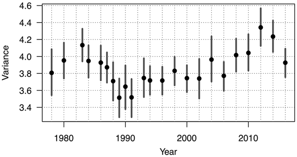
Variance in the General Social Survey question on preferences for government assurance of equitable wealth distribution. Error bars span 95% confidence intervals.

The core analysis of this GSS item is solely intended to assess whether it would be appropriate to assume that the variance in the underlying, micro-level, distribution from which the policy input is drawn is time-invariant. The bootstrap analysis and Breusch–Pagan test both provide evidence that the constant variance assumption is inappropriate in this case. A natural follow-up question, given the result from Wassef and Messih (1960), and its applicability to the study of policy change, is whether this GSS item exhibits leptokurtic change in the mean. It does not. The kurtosis in the change in the mean annual item value is 2.39. However, this results largely from the underlying distribution of this item, which is closer to uniform than normal, and the uniform distribution has a kurtosis of 1.8 (Sugiura and Gomi, 1985). This is a seven-point item without distinct tails, as the extreme points on the scale occur more frequently than most of the other five points. Indeed, the first value (1) is the mode. The mean annual kurtosis value, over the 23 years in the series, is 1.97, with a maximum of 2.14. If we consider the context of the year-wise micro-level distribution, we see that the distribution of the change in the mean has a higher kurtosis than the individual year-wise distributions.

Implications

Leptokurtic policy change is ubiquitous. What does this pattern tell us about the way in which policymaking outputs respond to policy inputs? When we observe leptokurtic policy change, we can reject the simplest form of the incremental policymaking model—that in which policy inputs are drawn from a normal distribution with stable parameters. What I have shown in the current article is that if the constant input variance assumption is relaxed, finding high kurtosis is not sufficient to reject an incremental model of policymaking. I should emphasize that I do not engage or present a challenge to any of the theoretical claims found in the literature on punctuated equilibrium in policymaking. Specifically, the results presented in the current paper do not speak to the process by which policymakers respond to streams of inputs that are too complex to perfectly reflect in policymaking. Policymaking may follow long periods that lack responsiveness to inputs, punctuated by periods of dramatic change in response to inputs. Policymaking may also follow a pattern of incremental change in response to bursty input signals. What I have shown is that to reject incrementalism through reference to leptokurtic policy change requires an assumption that the input signals have constant variance over time.

I recommend three pathways along which researchers could build upon these results in future work on punctuated equilibrium in public policy. First, realizing that measuring policy inputs is substantially more challenging than modeling outputs, the current study serves as additional justification for taking on that challenge. Second, in the case that measuring inputs is not possible or is prohibitively costly, I recommend that researchers develop theory regarding the distribution of inputs that addresses how variance will change over time. Theoretically informed characterizations of over-time variation in variance of inputs would make it possible for researchers to test changes in policy outputs against more complete and realistic null models. Third, in the case where it is not possible to measure inputs, or support a specific theory that accounts for over-time variation in variance, robustness checks should be conducted to changes and relaxations of assumptions regarding policy input distributions, following and building upon the example of Padgett (1980).

Based on the critique and results I present in the current paper, I echo the value of robustness in the context of evaluating theory through the analysis of distributional properties. Conventional theoretical models used in the study of policy change—Padgett (1980) aside—imply an exact distribution of the change in policy inputs—a normal distribution. Comparisons of incrementalism and punctuated equilibrium theory that are based on tests for leptokurtosis lack robustness to the distribution of policy inputs. Just as we seek robustness to alternative model specifications and measurement strategies in tests of theories that rely on differences in location, it is valuable to scrutinize tests involving other distributional properties for robustness regarding assumptions regarding the data generating process.