
Abstract
I reassess the argument by Tavits and Letki (2009) that in Eastern Europe in the 1990s and 2000s left-leaning governments were less likely to spend than right-leaning governments. I argue that the findings are most likely driven by time bias in their manifesto-based measurement of ideology. Starting in the mid-nineties, governments became artificially leftist, thus, the robustness of the relationship proposed by Tavits and Letki may be questioned. When adjusted for time bias, ideology does not influence spending in Eastern Europe. These findings have important consequences on the established literature linking ideology and spending. The findings also suggest that although manifesto-based measures of ideology have become widely used in time-series analyses, ideology scores at different times may not be comparable without adjustments.
A well-established literature has claimed a relationship between government ideology and government spending in Western Europe, with left governments expected to spend more (see Imbeau et al., 2001 for a review). In a highly referenced article, Tavits and Letki (2009, henceforth referred to as T&L) argue that this relationship does not hold for the countries of Central and Eastern Europe (CEE) in the 1990s. Quite the contrary, T&L argue that left parties in CEE were more likely to cut spending while in government.
In this paper I argue that the results in T&L may be driven by time bias in their estimates of ideology. When adjusted for such bias, the relationship in T&L disappears.
Specifically, starting from the mid-nineties parties in CEE were becoming increasingly “leftist” based on the Comparative Party Manifesto (CMP) measure employed by T&L. If this movement is driven by time-related bias, as opposed to changes in the parties’ true ideological positions, it has consequences for T&L’s analysis and conclusions. If there is a steady move towards the left, the parties (and governments) later in the time series will be on average to the left of parties (and governments) earlier in the time series, regardless of electoral results. If this left movement coincides with a period when governments are more likely to get their finances in order (late 1990s and early 2000s), the robustness of the findings in T&L may be questioned.
Time bias in measures of ideology has been recognised as a potential problem in time-series analyses, but until recently no methodological solution has been provided. An algorithm developed by König et al. (2013) however, provides such a solution. I applied this algorithm to the measure of ideology used in T&L and found the analyses with cabinet ideology adjusted for time bias did not confirm the relationship hypothesised by T&L. The statistical results were further confirmed in the qualitative analyses of Hungary and Poland – the two countries discussed at large in T&L (see Online Appendix 5). These qualitative analyses show how little the ideology of the government parties in these two countries mattered in their decision to spend; they also suggest that the process of EU accession constrained governments in the late 1990s and early 2000s causing reduced spending.
The findings have implications beyond CEE and suggest that when comparing ideological scores at different times researchers should be cautious. In the presence of time bias such scores should not be compared, or at least not with some additional adjustment, such as the one proposed in König et al (2013).
Cabinet ideology and spending in CEE: the argument in T&L
T&L argue that, contrary to the findings in the literature, cabinets in CEE in the 1990s were more likely to cut spending if they were of left rather than right orientation. This is because left parties had to prove their disassociation with the old socialist regime, and relied on a more stable and loyal electorate that would not punish them for the cuts.
To support their theory T&L provide qualitative assessments of government spending behaviour in Hungary and Poland, assessments that focus on the left governments between 1993 and 1997 and 1994 and 1998 respectively.
The main statistical analysis regresses total public domestic spending on government ideology in 13 former communist countries between 1990 and 2004 while controlling for a series of economic factors. 1 Additionally, T&L run the models with health spending and education spending as dependent variables. The main predictor, cabinet ideology, is a weighted average of left–right ideologies of all parties in the cabinet coalition, derived from the CMP dataset. As the use of existing methods to construct a left–right score (i.e. the RILE scale) to CEE has been shown to be problematic for CEE, T&L propose their own method summarised in Table 1.
The construction of the ideological left–right in T&L.

The results of the statistical analyses in T&L show a significant positive association between cabinet ideology and total spending, as well as spending on health and education.
The use of party manifestos to establish ideological dimensions of conflict has been established as a valuable tool. This method however has its shortcomings, among them the potential for cross-country and cross-time bias in the estimates (Franzmann and Kaiser, 2006; König et al., 2013). Here I focus on time-related bias. When comparing two parties at two different times that mention the same policy category to be included in a left–right measurement 10 times, the researcher assumes that the two parties defend the same position on a common scale. This assumption is questionable, as the two manifestos were written in different contexts. A British party in the 1960s might be more likely to use “leftist” promises than a party in the 1980s, even if they were to defend the same position on a latent left–right scale. Furthermore, the expectation that two British parties with identical ideological scores measured in the 1960s and 1980s spend the same when in power also need not hold.
In figures 1 and 2 I graph a series of yearly ideology averages (1992–2004) for the countries in T&L’s analysis. 2 Prima facie, the graphs suggest there may be time bias in the ideological measurement used by T&L. The average yearly cabinet ideology constantly slides to the left starting in the mid-nineties, as evidenced in Figure 1. This shift does not seem to be determined by electoral results (i.e. the election of social democrats or former communists), but rather by overall shifts in the political discourse. Thus, Figure 1 also graphs the average left–right placement of the parliaments in the 13 countries, which mirrors the government average graph accurately. In Figure 2 I re-graph the average government ideology but I replace the CMP-based measurement used in Figure 1 with one based on party labels. This measurement accounts for the average share of government seats held by parties labelled “left” in the CMP dataset. 3 The patterns observed in Figure 1 do not hold.

Average yearly cabinet and parliament ideology for the 13 countries in the sample- CMP-based measure.

Average yearly cabinet ideology in the 13 countries in the sample- label-based measure.
I remain agnostic about what may have caused such a leftist turn, as there may be multiple sources. Possibly, as time progressed, parties in CEE found it less damaging to include leftist promises in party manifestos, as these promises became less associated with the communist past. Also, redistributive promises may be related to the need to alleviate the negative consequences of economic reforms. Finally, the special way to measure left–right employed in T&L that gives weight to CEE-specific issues may also contribute to the bias (see Online Appendix 3).
A good way to illustrate the consequences of potential time bias is with the help of the two countries discussed at large in T&L, Hungary and Poland. According to T&L, the most drastic economic reforms in the two countries were taken under the left-leaning governments in power between 1994 and 1998 in Hungary and 1993 and 1997 in Poland. Following elections, these governments were replaced by conservative government coalitions. By all accounts (including T&L’s) in both countries there was a return of the political right. But this is not captured by the CMP data. Figure 3 graphs the left–right positions of the two sets of coalitions derived from the manifestos before the 1994 and 1998 elections in Hungary and 1993 and 1997 elections in Poland.
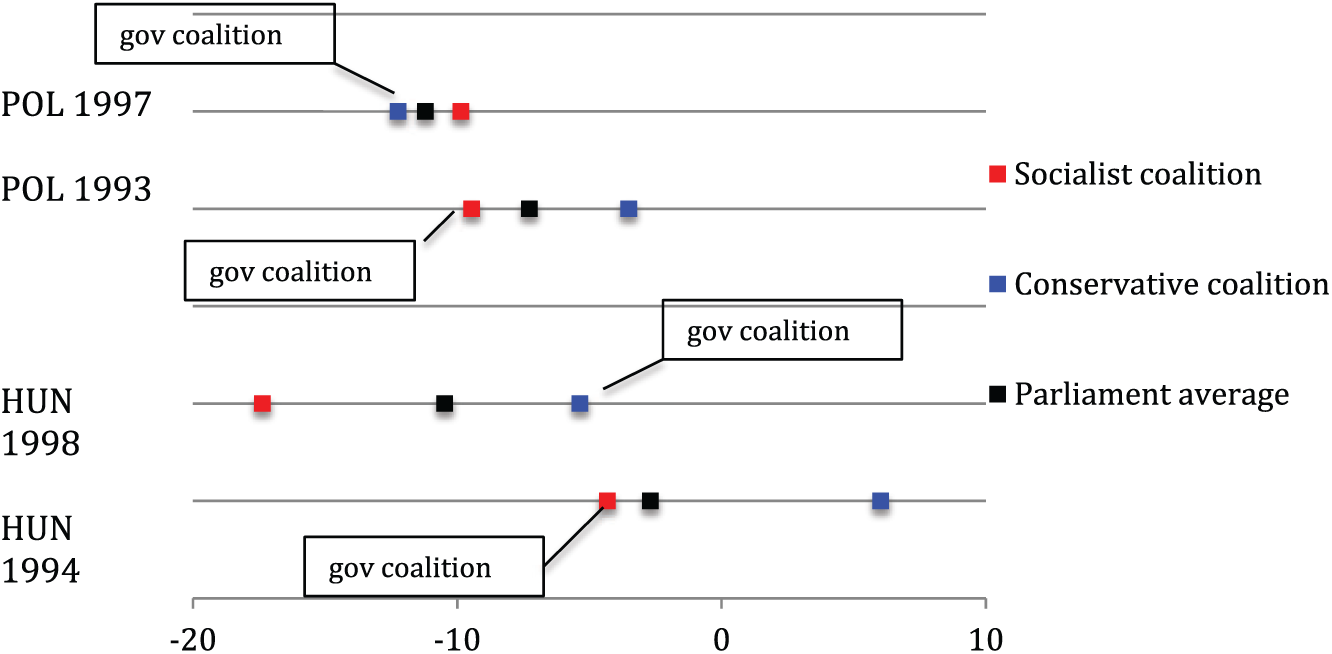
Average positions on the CMP-derived left–right of the socialist and conservative coalitions in Hungary in Poland in the 1990s.
Two observations emerge. First, as expected, the ideology averages of the parliaments in the two countries move to the left between elections. Second, despite the socialists being replaced by conservatives, this change is not captured by the CMP left–right measure. The conservative coalitions (based on label) that come to power in both countries in the second part of the nineties are ideologically to the left (based on CMP) of the socialist coalitions previously in power. In the dataset the left coalitions that T&L praise for neo-liberal reforms are ideologically right when compared with the coalitions that followed.
If this pattern applies to the other countries in the sample – and the evidence in figures 1 and 2 suggests it does – then the overall results may be biased. In the following section I provide statistical evidence of ‘left’ bias in most countries. The governments in CEE seem to shift towards the left as time progresses, starting in the mid-nineties.
The patterns in Figure 3 show an inconsistency between the qualitative story in T&L and their measurement, but also point more generally to the issue of time bias. Looking at the Hungarian case for instance, in each of the two years (1994 and 1998) the ideological distances between the two coalitions are similar, only both move to the left in 1998. This move may reflect a genuine shift to the left of the entire party system that would be captured by other measurements such as expert surveys. But a drastic move like the one suggested in figures 1 and 3 may also be caused by a switch in general discourse that makes the manifestos of all parties more likely to include leftist promises. Such a shift would not be captured by other measures. To the extent that this second cause of leftist drift is present in the data, the expectations about differences in government behaviour (more or less spending) need not hold. These artificial shifts towards the left or right, if present, are accounted for by the algorithm developed by König et al. (2013).
Time-bias adjustment using the Manifesto Common Space Scores estimator
The MCSS (Manifesto Common Space Scores) is an algorithm based on Bayesian factor analysis motivated by the need for comparability of measures across party systems and across time.
To construct their algorithm König et al. (2013) followed Lowe et al. (2011) and recoded the CMP data into a logit scale with the formula

where R and L represent the number of right and left sentences respectively. Here
To account for potential time- and country-specific effects, the MCSS includes two additional parameters for country bias and time bias. These parameters are estimated using bridge observations. First, the parameter for country-specific bias is computed as the difference between the position of each party in its manifesto for the first European elections and the previous national elections. This procedure relies on what the authors call ‘the zero hour hypothesis’, that is, the assumption that ‘parties took the same position in their first EP election as in the previous national election’ (König et al., 2013: 5). Second, to account for potential time bias within countries König et al. (2013) assume that the party that added the most votes in an election (compared with the previous election) keeps the same ideological position in the following election. Differences between these two are assumed to be bias.
The actual left–right scale was not defined inductively post-MCSS estimation. Instead, König et al. (2013) used the Chapel Hill Expert Survey data (1999–2006) and/or the Eurobarometer survey as ideological priors to compute means and variances in the left–right scale for each of seven party families. 4 These were in turn set as intercepts and variances for all parties belonging to that particular family. Thereafter, the trajectory of the parties was modelled using Legendre polynomials.
The model was implemented in JAGS (Plummer, 2003). The results of the estimation in König et al. (2013) showed both high validity and robustness to different specifications.
In the following section I employ the MCSS algorithm to create a common ideological space for Eastern Europe in the 1990s and early 2000s; I then compute yearly measures of average government ideology adjusted for time bias and use them to re-test the main argument in T&L. To create the common ideological space I draw on CMP data (1990–2016) from 20 Eastern European countries that satisfy the criteria in T&L for inclusion in the analysis. 5 In keeping with the analysis in T&L, I only use the CMP categories in Table 1.
To create ideological priors for party families in Eastern Europe in the 1990s and early 2000s I used the Consolidation of Democracy in Central and Eastern Europe public opinion survey, 1990–2001. To implement the model I used the exact parameters set in König et al. (2013). 6 The Gelman and Rubin (1992) convergence diagnostic support this choice. More details about the issues related to the application of the MCSS estimator to CEE in the 1990s and early 2000s can be found in Online Appendix 1.
Figure 4 graphs the value of the time-bias parameters estimated by the MCSS algorithm for each of the 13 countries in the dataset, together with the 95% Bayesian credible interval. 7 Negative values represent leftist bias. The graphs support the claim from figures 1–3 that there is a time bias starting roughly in the mid-nineties. All elections post-1996 that show bias, have left bias. Furthermore, each of the 13 countries has at least one election after 1996 where there is evidence of left bias.

Time-bias parameter: posterior density summary of the time-bias parameter, and 95% Bayesian credible interval.
Once the ideological space was created, I computed adjusted yearly measures of cabinet ideology and re-ran the main models in T&L. The results of the statistical analyses are reported in Table 2. For brevity, I only report the coefficients and standard errors for the variable of interest, cabinet ideology. Results including all controls are reported in Online Appendix 2.
Cabinet ideology and spending behaviour in Central and Eastern Europe (1990–2004).
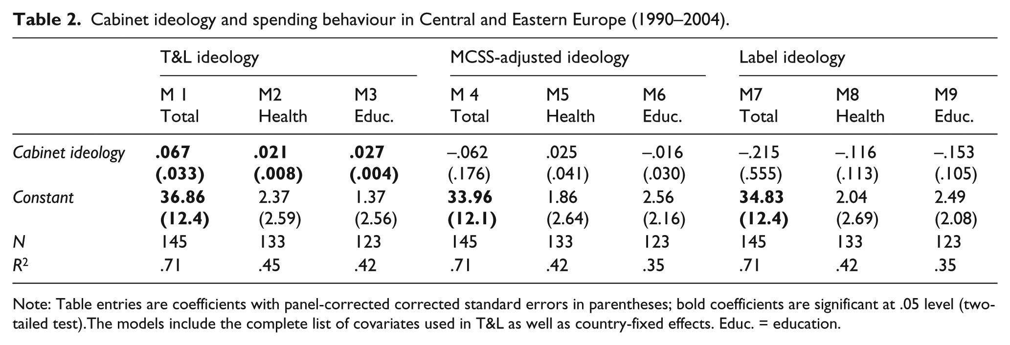
Note: Table entries are coefficients with panel-corrected corrected standard errors in parentheses; bold coefficients are significant at .05 level (two-tailed test).The models include the complete list of covariates used in T&L as well as country-fixed effects. Educ. = education.
In models 1–3 of Table 2 I replicated the main results in T&L. The dependent variable was the difference in spending from the previous year. Model 1 reports the results of the main statistical analysis in T&L, with total spending as the dependent variable and cabinet ideology unadjusted for time bias. The coefficient for ideology was only slightly different from that reported in T&L but positive and significant, confirming the main finding in T&L that total government spending increases during times of right-leaning governments. In models 2 and 3 I replaced overall spending as dependent variable with spending on health and education respectively. Again, the results were not significantly different from those in T&L.
Models 4–6 re-tested the main analyses in T&L with cabinet ideology adjusted using the MCSS algorithm. The results did not confirm the relationship between cabinet ideology adjusted using the MCSS and total spending, or spending on health or education. For two of the three models (with total spending and education respectively) the sign of the coefficient was in the opposite direction of the results in T&L; the non-results are therefore unlikely to be driven by a noisier measure that simply increases standard errors. Additionally, in Online Appendix 2, Table A4, I report the results of statistical tests with no country-fixed effects. The coefficients for all three dependent variables were negative, and statistically significant for total spending. In models 7–9 I used a label-based measure of ideology that measured the proportion of cabinet seats held by left parties. This label-based measure was insensitive to time-driven bias, albeit less precise, as argued by T&L. Again, the results in T&L did not hold.
Thus far the analyses have suggested a left bias among the parties in Eastern Europe as we move through the nineties. Once adjusted for this time-related bias, the main findings in T&L do not hold. This suggests that the progressive move towards the left is associated with a move towards fiscal responsibility later on in the time series, which drives the findings in T&L. Explaining the causes of such a shift is beyond the limited scope of this research note.
If one were to speculate however, the process of accession to the EU emerges as a serious potential explanans. Ten of the 13 countries in the sample were involved in this process. The pressure on the EU candidates to cut spending came from the need to meet both the Copenhagen criteria and the Maastricht convergence criteria, as detailed in Online Appendix 4. The qualitative re-assessment of government spending behaviour in Hungary and Poland throughout the nineties in Online Appendix 5, supports this expectation about the role of EU conditionality.
The use of the MCSS-adjusted measure may raise some questions, which I address here. First, the influence of time bias on the results is contingent on the comparisons among governments at different times in a country-fixed effects environment, and should not be much of an issue in a cross-sectional environment. In one of their robustness tests, T&L control for time-fixed effects on top of country-fixed effects. This, however, does not fix the problem of time bias, as the inclusion of country- and time-fixed effects yields a coefficient that is an average of both across-country and within-country (and in our case subject to bias) effects, as demonstrated in Kropko and Kubinec (2017).
Second, there is a question of whether the slide to the left graphed in Figure 1 is indeed reflective of time bias or of real changes in the true ideological positions of the parties. This question is important for any future works that intend to use the adjustment in König et al. (2013). For the data used in T&L the MCSS algorithm suggests there is time-related bias, but the conclusion is based on the assumption that parties that win elections keep the same ideology in the following elections, an assumption that may be questioned. A solution to such a dilemma is triangulation, trying to confirm the patterns observed in the CMP-based measures of ideology with other measures such as the placement of parties by experts or public opinion survey respondents. For my purposes I was able to find two expert surveys that include some of the countries under analysis at two important time points: (a) the survey run by Huber and Inglehart (1995), which was sent out to experts in the winter of 1993; and (b) the 2002 Chapel Hill Expert Survey. Seven of the countries in T&L were included in both surveys. For these countries I computed parliament ideology averages, similar to those graphed in Figure 1, but only from two time points, 1993 and 2002. 8 To allow comparison with the measures derived from CMP (Figure 6) the expert scores were standardised. These standardised ideology averages, graphed in Figure 5, did not confirm the slide to the left present in the CMP-based measure. If anything, the average ideologies of parliamentary parties in the seven countries seemed to slide slightly to the right.
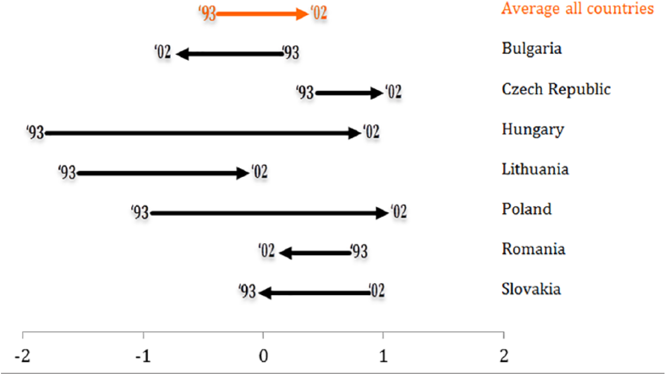
Average parliament ideology for seven countries in the sample at two time points: standardised measures derived from two expert surveys.
In Figure 6 I graph the standardised average ideologies of parliament parties for the seven countries at the same two time points, derived only from the unadjusted CMP-measures used in T&L. A clear slide to the left in each country can be observed. The graphs in figures 5 and 6, together with the MCSS diagnostics in Figure 4, give strength to the claim that the ideology measurements in T&L suffer from leftist time-bias.

Average parliament ideology for seven countries in the sample at two time points: standardised measures derived from manifestos.
Third, the results disconfirm the findings in T&L but do not support the opposite relationship expounded in the previous literature. The lack of any relationship between government ideology and spending behaviour is most likely explained by the constraints faced by the governments in CEE in the 1990s brought by both their transition to a market economy and EU membership that rendered their predispositions irrelevant. Additionally, the fact that the main axis of political competition in some Eastern European countries is likely to be associated with visions of the nation rather than redistribution (Coman 2017; Rovny, 2014, 2015) may also provide an explanation for the non-findings.
Conclusion
This paper was driven by a seminal work on government spending in CEE in the 1990s by T&L, which argues that left governments were more likely to cut spending, or to be ‘right’. I argue that the results were most likely driven by time bias in the measurement of ideology.
Although written as a response to a seminal work, this paper has broader consequences for the use of manifesto-based measures of ideology in time-series analyses. One of the most touted benefits of manifesto-based measures is that they allow us to travel back in time to create left–right measures from decades ago. But one has to remember that political vocabulary changes, and what is leftist language in one historical context, may not be in another. As such, ideological scores obtained at different times may not be comparable, or at least not without some adjustments such as the one proposed by König et al. (2013).
This certainly seems to be the case in CEE in the 1990s and early 2000s, a period from which we have little to no data from alternative sources such as expert surveys. Because of this, the use of manifesto data emerges as an attractive/necessary solution; the evidence of time-related bias presented in this paper however, should caution researchers.
Second, the paper has implications for the literature on government ideology and spending. T&L’s findings challenge the well-established association between left governments and spending. Here I show that these findings are likely to be driven by time bias in the ideology estimates, and that once adjusted for this time bias their results do not hold.
Supplemental Material
appendix#3 – Supplemental material for When left or right do not matter: Ideology and spending in Central and Eastern Europe
Supplemental material, appendix#3 for When left or right do not matter: Ideology and spending in Central and Eastern Europe by Emanuel Emil Coman in Research & Politics
Footnotes
Acknowledgements
I would like to thank Ken Bennoit, Raimondas Ibenskas, Liesbet Hooghe, Gary Marks, Marius Radean for valuable comments on earlier versions of the paper.
Declaration of conflicting interests
The author(s) declared no potential conflicts of interest with respect to the research, authorship, and/or publication of this article.
Funding
The author(s) received no financial support for the research, authorship, and/or publication of this article.
Supplementarl materials
Notes
Carnegie Corporation of New York Grant
This publication was made possible (in part) by a grant from the Carnegie Corporation of New York. The statements made and views expressed are solely the responsibility of the author.
References
Supplementary Material
Please find the following supplemental material available below.
For Open Access articles published under a Creative Commons License, all supplemental material carries the same license as the article it is associated with.
For non-Open Access articles published, all supplemental material carries a non-exclusive license, and permission requests for re-use of supplemental material or any part of supplemental material shall be sent directly to the copyright owner as specified in the copyright notice associated with the article.