Flows of air,flows of electrons

Abstract

Today’s comprehension of the global climate and other elements of the Earth system is synonymous with the computation of their dynamic processes in digital machinery. Given their central role in assessing the criticality of the planetary- and epoch-scale changes currently underway, it seems crucial to fathom this conceptual and material basis of the Earth (system) sciences. This is what the field of historical epistemology has to offer. It explains how certain forms and formattings of knowledge came to be (and why others did not) by helping to understand the historical path dependencies, relationships, limits, and possibilities that frame a particular way of knowing. How then and under what circumstances became geophysical phenomena and their time-based evolution represented by digital and electronic media? This paper seeks to contribute to this historical analysis by revisiting the emergence of atmospheric motion modeling until the middle of the 20th century. It argues that the close association between atmospheric flows and electron currents was not just merely a practical consideration but one that rested on longer traditions in which fluid and electromagnetic phenomena intimately shared epistemic and technological contexts as well as formulas. Highlighting the electrophysical context from which Vilhelm Bjerknes derived his famous circulation theorem, that, in turn, led to the rise of modern atmospheric science, the paper attempts to make the theoretical and practical proximity, if not sometimes community, of hydrodynamics and electrodynamics more palpable and legible. The essay describes and interprets a long-standing and quite productive back-and-forth relationship between these two seemingly different physics-based realms, in which experimental electrophysics informed theoretical geophysics and electronics opened up ways for numerical experiments on fluid motions.

“Aethers were invented for the planets to swim in, to constitute electric atmospheres and magnetic effluvia, to convey sensations from one part of our bodies to another, and so on, till all space had been filled three or four times over with aethers.”

Maxwell (1878: 763)

Introduction

The comprehension of a changing global climate rests on the numerical representation of the eternal flows of two elemental media: the earthly envelope of air and the vast body of ocean waters. This focus is not surprising, given the fact that the atmosphere and global ocean are the essential geofluids that receive, store and distribute solar heat and by doing so keep this planet habitable and metabolic (Williams and Zalasiewicz, 2022). In its most sophisticated form this representation-by-calculation is performed in an epistemic architecture called General Circulation Models (GCM). The term “general circulation” here refers to the large-scale flows of the planetary atmosphere, the constant evolution of which is three-dimensionally resolved by GCMs. Similar dynamical models that simulate the circulation of the oceans are often coupled with atmospheric models, but the original focus lies with the upper flows of air encircling the globe.

For many decades GCMs have been, and to a large extent still are, conceptually and methodologically coextensive with the simulation of the sensitivity to specific forcings, such as an increase in greenhouse gas concentrations, and the potential evolution of the global climate, a fact that sometimes inspired the acronym to refer instead to a “global circulation model” (Randall et al., 2018) or simply “global climate model” (Edwards, 2010: 141). GCMs can be considered as the basic workhorses of the climate community and have constituted the central epistemic pillar of all the different reports of the Intergovernmental Panel on Climate Change (IPCC) so far. In recent times, and in tandem with constantly increasing computing power, they have gradually extended outwards to incorporate further modules such as vegetation cover and geochemical fluxes, essentially becoming fully-fledged Earth System Models (ESM). ¹ The gradual addition and further integration of climate-relevant Earth system components is part of the programmatic objective of climate modeling to evolve into an Earth system science that takes greater account of the interaction of planetary subsystems and their different time scales, with increasing efforts to link these up with different modeling frameworks that not only detail biophysical processes but also focus on the co-evolutionary dynamics between human societies, the technosphere, and the rest of the Earth system (e.g. Donges et al., 2020).

In a very coarse sense, unpacking this epistemic architecture is equivalent to an exercise in historical genealogy. To put it very crudely: Both architecturally and historically, today’s Earth system models consist of atmospheric GCMs, whose architectural as well as historical core in turn consists of numerical weather prediction models. Going another level deeper, these weather models are driven by equations that describe the mechanics of moving fluids. The innermost part of this epistemic Russian doll system thereby is governed by a set of nonlinear partial differential equations, the so-called “primitive equations,” originally devised by the Swiss-German mathematician Leonhard Euler in the mid-18th century during the early days of analytical mechanics. ²

The genesis of climate modeling and its origin in dynamic meteorology and numerical weather prediction is nothing new to historians of atmospheric science and has been described many times (e.g. Edwards, 2010; Fleming, 2016; Gramelsberger, 2010; Harper, 2008). These origin stories have also become part of the internal folklore of the discipline, as indicated by the reflections of many protagonists themselves (e.g. Cressman, 1996; Smagorinsky, 1983; Thompson, 1983; Wiin-Nielsen, 1991).

It is still worth summarizing this story. Commonly, it does not start with Euler but with a programmatic paper by the Norwegian physicist and meteorologist Vilhelm Bjerknes published in 1904. It stated that the ultimate, though hardly attainable, goal of a physics-based meteorology was to calculate the future state of the weather from the present state by integrating the aforementioned equations of fluid motion (Bjerknes, 1904b). Several developments in dynamic meteorology, particularly in Austria, foreshadowed a broader and paradigmatic replacement of a meteorology plagued by unruly empiricism and a turn to “rational” physical-exact methods of computing the larger-scale features of the fluid envelope of the Earth through which the weather develops (Coen, 2018). But it was the Norwegian physicist who stripped the problem down to its bare hydrodynamical and thermodynamical fundamentals (Fleming, 2016; Friedman, 1989; Gramelsberger, 2009; Vollset et al., 2018). He regarded weather prediction as a problem that would be solved if one were able to project (observed) initial values forward in time by integrating the primitive equations. As Bjerknes also knew, however, a proper integration was simply unfeasible due to the nonlinearity involved, by which every future state of one of the basic variables (velocity in all three directions, density, pressure, temperature, and moisture) is dependent on all the other ones. His suggestion was to shrink the complexity by proposing the simpler Euler form instead of the more realistic Navier-Stokes equations. ³ But this did not do much to ease the fundamental dilemma. Bjerknes was well aware that he had to abandon any hope of having his program become a reality. Instead, he worked over the coming decades with a team of assistants in what has come to be known as the “Bergen School” on devising mixed numerical and graphical methods—and, indeed, graphical integration machines—to construct the dynamic progression of weather systems on maps.

Still, during World War I British meteorologist and pacifist Lewis Fry Richardson made an attempt to deal with the problem of weather forecasting through direct integration of the primitive equations (Lynch, 2006; Richardson, 1922). It utterly failed: After many months of dreadful calculations of the pressure tendencies of a fair-weather morning of May 20, 1910 over Southern Germany, his resulting pressure fields were so high, that they would have more or less turned all humans living underneath them into (constantly vomiting) quadrupeds. For his experimental hindcast Richardson had employed a numerical scheme, that is, an approximative and algorithmic approach with actual truncated numbers. Here, the motion of the continuous medium air, represented in its infinitely small totality by the differential equations, is discretized into finite differences projected on a spatial grid, wherein each variable at every grid point and in every time step is solved arithmetically before the next one is taken up: an immensely tedious process for a human computer, but a straightforward, that is, programmable, task for a machine to perform, especially if this machine works at the speed of flowing electrons.

This is exactly what was accomplished a few decades later in the United States. In 1945 the Hungarian-born mathematician John von Neumann initiated a project at the Institute for Advanced Study (IAS) in Princeton to build a universal electronic computer to solve a range of problems that can only be treated numerically (Goldstine, 1973). The so-called IAS machine was set to become the template for a whole generation of modern computers; its original inspiration, however, arose from the challenges associated with the mathematical simulation of the hydrodynamic processes that occur immediately prior and after the explosion of an atomic bomb (i.e. shock waves). After the war, von Neumann became soon captivated by the application of the computer to a yet entirely different scale of hydrodynamic behavior, namely that of the circulation of the free atmosphere (i.e. planetary waves). By the summer of 1946 he managed to add a Meteorology Project to his Electronic Computer Project, in effect merging the development of the computer with the development of appropriate equations for atmospheric analysis and weather prediction (Harper, 2008; Rosol, 2015). Over the following years a highly unusual group of meteorologists, mathematicians and electrical engineers worked in a small building just off the institute’s grounds, practically fusing, both on the level of laboratory space and personal interaction, electrical engineering with atmospheric science (Dyson, 2012).

During its initial phase, the project was riddled by many personal and technical obstacles, of which the development of appropriate electron tubes for digitally storing the numbers during a calculation was probably the most daunting. Due to the unavailability of the memory tubes, the first test for a numerical reconstruction of a weather episode, that is hindcast, with a much simplified atmosphere took place in 1950 on the Electronic Numerical Integrator and Computer (ENIAC) located at the Aberdeen Proving Ground in Maryland (Charney et al., 1950; Lynch, 2008). Once the IAS machine finally became operational in 1952 the once failed “Bjerknes-Richardson approach” (Petterssen, 1957: 115) soon became a viable competitor to the various statistical, synoptic-climatological, type and analog, or regression and extrapolation techniques employed by the forecasters to deal with the data mess and the stubborn intractability of weather prediction. However, a different use of the numerical model opened up shortly before the Princeton group disbanded in 1956. One of its members, Norman Phillips, undertook a numerical experiment to model the appearance of the patterns of the large-scale atmospheric circulation as such from a planetary state of rest (Phillips, 1956). Here, no initial data of a given meteorological state, but the overall boundary conditions (e.g. the temperature gradient between equator to poles or the vertical stability lof the atmosphere) in conjunction with empirical and physical laws formed the crucial parameters for testing whether the computed flow patterns would, after a considerable spin-up time, start resembling the gross features of the atmosphere. A new branch of experimental computerized investigation developed from Phillips’ numerical experiment: global climate simulation. This new, data-intensive science then became a major catalyst for the establishment of the technical and institutional infrastructures and international programs that defined the structural build-up of Earth system science during the Cold War (see e.g. Aronova, 2017; Edwards, 2010; Rispoli and Olšáková, 2020).

As mentioned, this particular genesis story is now another classic in the history books. Yet it is one that is, in most cases, either told through the lens of the development of numerical weather prediction (with almost no mentioning of the technological aspects of developing the electronic computer) or through the lens of early computer engineering (with only a short nod to the meteorological aspects). The “grand challenge” for a more comprehensive historical epistemology therefore would be to connect the two, the history of understanding the flow of air (through simulating it) and the history of understanding electric currents (through engineering them). The history of planetary, and therefore data-intensive science, is of course populated with electric/electronic telecommunication media of all sorts. Paul Edwards convincingly showed how its data-centric knowledge infrastructure is interspersed with a whole suit of different models (Edwards, 2010). Beyond these infrastructural considerations, a further provocation would be to look for historical reciprocities, if not epistemic analogies or even isomorphisms, between atmospheric processes and the processing of electric signals: in concepts and verbalizations, but also in concrete technical architectures and materializations. If computer simulations of the climate and the Earth system indeed “established a fundamentally new world-related-to-actor relationship, in that it is possible to experiment projectively with the production specifications themselves” (Gramelsberger, 2010: 278, author’s translation) then these production specifications have not only epistemic value but also a broader valence. They beg the question: what expansive or limiting factors, what political and esthetic ramifications, and which conceptual pathways and technological path dependencies were formed through relating the planetary to concepts and materialities of electric/electronic signal processing? Or, vice versa, how conceptualizations of the fundamentally unstable flows of the world medium atmosphere precipitated into the electric/electronic surroundings which now, in turn, fundamentally shape our (no less unstable) planetary life (Creutzig et al., 2022; Rosol, 2022)?

Such book-length study, of course, cannot be accomplished here in a stipulated short article. What I aim to do, instead, is twofold. In a first step I revisit the origin story of Vilhelm Bjerknes’ programmatic paper and show what this has got to do with the claimed epistemic proximity of the scientific comprehension of the atmosphere as a medium and scientific uses of electrical media of Bjerknes’ time. I follow this with some wider historical and epistemological reflections on the shared legacy and co-productive episteme of hydrodynamical and electrical flow, which influenced, in quite material ways, their engagement in addressing the unstable and unpredictable in later computer modeling.

A model globe

There are multiple, and sometimes even time-honored ways of modeling the planetary. The Norwegian Museum of Science and Technology in Oslo houses a somewhat modest mechanical globe (see Figure 1). It consists of a simple glass sphere in the center of which another sphere can be set in rotation via a rod. On the inner sphere, different colors demarcate different areas, three per hemisphere, a clue to what it is for. The areas separated from each other apparently mark the zones or cells of atmospheric circulation of our planet: In red the tropical Hadley cell, in which the trade winds prevail; gray the unusually narrow Ferrel cell, depicting the well-known westerly wind zone of temperate latitudes, and in the same color a last cell at the respective polar caps. Another indication of the purpose of the apparatus are the traces of wax found inside the globe. A steady drive of the inner sphere might have gradually produced a viscous, more or less stationary flow pattern in the liquid wax in the pretty oversized layer between the inner sphere and the glass. The globe was apparently intended to provide a grossly simplified scale-model for the flowing motions of air that envelop our planet: the general circulation.

Figure 1.

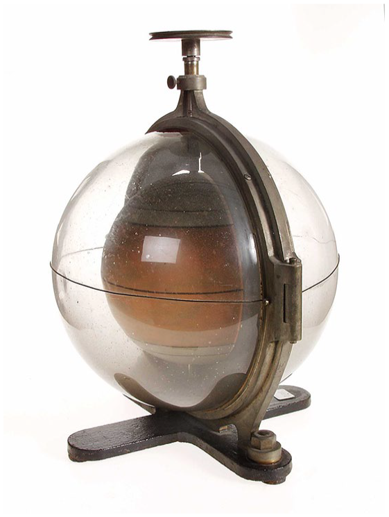
A late 19th-century scale-model of the general circulation (credit: Norsk Teknisk Museum, cataloged object 12179.).

From what is known, the model atmosphere was commissioned by the Christianian (i.e. Osloensar) physicist Carl Anton Bjerknes and was created sometime between 1898 and 1903. ⁴ It was probably Carl Anton’s attempt to model the geophysical implications of a new theorem that his son, Vilhelm, had recently developed. It dealt with the sudden emergence of vortices in fluids at the boundary surfaces between volumes of different densities and pressures within that fluid (Bjerknes, 1898). Until then, the authoritative vortex theories of Hermann von Helmholtz and William Thomson (Lord Kelvin), two of the most influential physicists in the second half of the 19th century, were based on ideal fluids that were either completely incompressible and homogeneous, or so conditionally compressible and heterogeneous that they rapidly become homogeneous at constant pressures (Helmholtz, 1858; Thomson, 1869). This homogeneity is referred to as “barotropic,” meaning that a fluid’s density is directly proportional to its pressure. This simplifying assumption resulted in a strict conservation of vortices: they could neither form nor decay but simply be or not be. Vilhelm Bjerknes’ theorem took its departure from the opposite, the “baroclinic” stance: in an inhomogeneous, compressible fluid, vortices can arise practically as if from nowhere, simply because of a varying density distribution, which—and this is what is special—is not a function of pressure alone, but can also be related to other variables like temperature and humidity. Hence, a circulation is produced everywhere where the mobility vector, responsible for the translatory motion of a parcel of air or water, is not the same as the pressure gradient. Which is, basically, everywhere: “We live at the bottom of a baroclinic atmosphere along the shores of baroclinic oceans,” as James Fleming aptly put it (Fleming, 2016: 25).

The mechanical globe was meant to show and study how such vortexes arise. One might therefore be inclined to think that the general-circulation model globe is part of the tradition that leads from Bjerknes to the eventual general circulation models, that is, from the scale model to the numerical one. But that would be wrong. Not only is the history more complex—this is always the case! No, Vilhelm Bjerknes probably never used the globe; the creation of the device was due to a misconception. That a consistent flow pattern resembling the dynamic features of the Earth’s atmosphere may have been established within the three cells is quite unlikely. The actual source and scientific background of Bjerknes’ preoccupation with the topic of large atmospheric flows around the Earth, of planetary waves and weather fronts, was instead something else: the tiniest effects of hydrodynamic and electromagnetic interaction. The dynamic treatment of the atmosphere gained its particular epistemic shape from the analogy—or even imagined identity—of hydrodynamics and electrodynamics and hence the useful phantasm of a force-carrying aether.

Attractive analogies

By training, and by mindset, Vilhelm Bjerknes was not a meteorologist but an experimental and theoretical physicist—one who worked, more so, in the service of his father (Bjerknes, 1933). For decades Carl Anton Bjerknes had dealt with a central concern of 19th-century physics in a way that was as simple as it was subtle. With an amazing inverse analogy between hydrodynamic and electromagnetic forces, as demonstrated in an ever more refined experimental arrangement, he hoped to prove the spatial plenum and mechanical agency of a luminiferous aether. According to Homer and other ancient Greek luminaries, the αἰθήρ (aether) was the “celestial blue”: a kind of rarified air, windless, that operates as a finest, space-filling, and translucent medium in which the planets swim (Kurdzialek, 1971: 599). The term became a backbone for 19th-century physics and an absolute frame of reference for all physical phenomena, and in particular so for the mathematical formalization of the equivalence of electrical and magnetic phenomena through the eminent Scottish physicist James Clark Maxwell (Maxwell, 1878). In this vein, Carl Anton wanted to make all Newtonian assumptions about action at a distance unnecessary and to put the whole of electrodynamics on a mechanical, that is, theoretically solid and comprehensible, basis. Fluid-mechanical representations of attractive and repulsive forces were to help demonstrate such contiguous actions going on in the aether.

What did these models look like? Figure 2 gives a first indication. Two elastic rubber balls were suspended in a tank filled with a fluid usually specified as plain water. Then, by means of a drive wheel, two tie rods were moved back and forth, periodically pushing in or pulling apart the membranes of two larger rubber drums, so-called “pulsators.” The resulting alternating air pressure in these drums was fed through a tube to the spheres, causing them to contract or expand. An astonishing effect was observed: When the pulsations were in the same phase, the two spheres seemed to attract each other, and when they were in different phases, they seemed to repel each other. This ominous force also appeared to be extremely rule-governed. It showed that the supposedly remotely acting force between the two elastic spheres was proportional to the product of the two pulsation intensities and decreased inversely to the square of their distance (Bjerknes, 1880).

Figure 2.

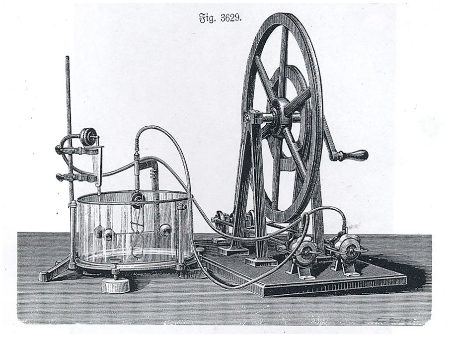
One of Bjerknes’ water tank experiments demonstrating attractive and repulsive phenomena (credit: Frick, 1905: 1433.).

Now, such a law-like effect is not just any phenomena, but the one defined by Charles Augustin de Coulomb for the attraction and repulsion between electric charges or between magnetic poles, respectively. And here then is also the analogy: The balls in their water bath behaved like electrically charged bodies or like magnets. However, they did this in the opposite way. While opposite charges and opposite magnetic poles attracted each other, different pulsations let the spheres in their water bath repel each other. Bjerknes called the forces in play here “hydroelectric” or “hydromagnetic.”

With this one experimental arrangement, however, the analogical reservoir was not yet exhausted. By exchanging the pulsations by so called “oscillations” he reached detailed reproductions of the effects between two complete magnets with all their different attracting, repelling, shifting, and rotating force effects. No longer periodic changes of volume but periodic changes of position of a sphere caused an apparent effect of “hydromagnets” moving uniformly in water.

With their bathing rubber balls Carl Anton and Vilhelm Bjerknes hit straight into the heart of the aether debate of the 19th century. The precise reproduction of the remote forces of electrostatics or permanent magnetism by quite obviously mass-moving forces seemed to correspond to Maxwell’s presupposition of an incompressible medium that carries all mechanical forces in a miraculous way—even if only inversely. The Bjerknesses had proved nothing, but with the power of visualization they succeeded in demonstrating a quasi-magical act of correspondence.

More of such surprising effects were in the making. After many failed attempts the young Vilhelm managed to amplify the microscopic movements of the fluid triggered by the pulsating or oscillating bodies and, with the help of an installed brush, obtained, in his own words, “complete, automatically drawn images of the flow fields” (Bjerknes, 1933: 152). The expected result of this self-drawing glass painting was a striking identity with the field lines of magnetic forces (see Figure 3). The vibrational lines formed the same figures as magnets; the drawn hydrodynamic fields yielded the same geometrical structure and kept the same direction as the known magnetic fields made visible by scattered iron filings.

Figure 3.

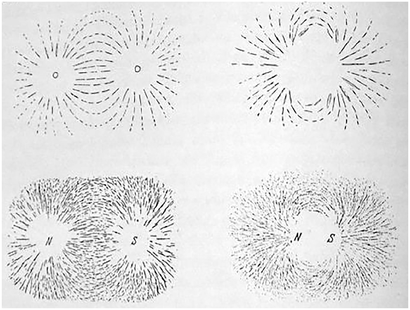
Comparison between the hydrodynamic lines drawn by pulsating rubber balls and magnetic lines of force (credit: Bjerknes, 1933: 154).

With the pulsating or oscillating spheres only figurative analogies of electrostatic and magnetic fields had been created. A field around the—significantly more contemporary—electric conductor looked different, exhibiting circular lines around a cross-section. And so father and son Bjerknes changed their arrangement, now immersing rotating and oscillating drums or cylinders in a bath of a viscous liquid (sometimes just syrup) and again obtaining in the same painterly way their “hydromagnetic” field lines of force analogous to the conductor.

From experimental electrophysics to theoretical geophysics

Vilhelm Bjerknes graduated in mathematics and physics in 1888 and a scholarship allowed him to go abroad for 2 years. First a year in Paris, where he followed in particular the lectures of Henri Poincaré on electricity and optics. Then in 1890 Bjerknes went to Bonn for an internship in Heinrich Hertz’s newly occupied laboratory. With his recent successes in generating electromagnetic waves, Hertz had experimentally confirmed Maxwell’s theoretical foundation for electromagnetism and thus not only provided the basis for the development of wireless telegraphy and radio, but spurred another wave of aether frenzy. With great zeal, Vilhelm set out to place the resonance phenomena of electromagnetic waves on a theoretically and experimentally safe footing, that is, to clarify and secure their mechanics quantitatively—just as he had done before with the hydrodynamic resonance phenomena in Christiania.

Back there, a year later, Vilhelm continued to work on resonance problems while also restarting his work on hydrodynamic analogies and searching for the medium responsible that would make electrodynamics and hydrodynamics not just analogous but identical in some way. During the theoretical reappraisal of the cylinder experiments it occurred to him to replace the purely geometrically defined solid bodies by geometrically analyzed fluid ones. This gave him justification to consider the hydrodynamic fields like electromagnetic fields, both outside and inside the moving bodies. The hydrodynamic geometry was thus applicable to the whole system, including the drums, with the difference that henceforth it was a question of two “fluids” of merely different density and compressibility meeting at a boundary surface where the lines of force break (Bjerknes, 1904a).

In 1897 this insight led Vilhelm Bjerknes to the formulation of his famous circulation or vortex theorem that dealt with the emergence of vortexes at the boundaries of different densities. Two years earlier he had become professor of applied mechanics and mathematical physics at Stockholm University, and it was there that he started to analyze line-bands, projections of surfaces of same pressure (the known “isobars”) and same specific volume, the reciprocal of the density (“isosters”). The isobaric and isosteric lines crossing each other now resulted in a series of curved-quadrangular parallelograms, or, when viewed three-dimensionally, tubes, which Bjerknes called solenoids. Bjerknes took this term directly from the vector analysis of electromagnetic fields in the tradition of Oliver Heaviside and Willard J. Gibbs; however, electromagnets in the form of a conductor coil, which enclose a hollow cylinder, and with which he experimented in Bonn, are also just simply called solenoids. The graphically constructed solenoids, which enclose spaces of unit density and unit pressure, were exactly the discontinuous surfaces encountered in the previous cylinder experiments. The numerical number of solenoids gave a concrete measure for the vortex acceleration: the more solenoids the stronger the rotational motion within a translational motion of a fluid.

In all of this, Bjerknes was still only concerned with theoretical physics. His vortex theorem assumed natural fluids, but remained abstract. Soon, however, he presented it to his geoscientifically minded colleagues in Stockholm: well-known figures such as Svante Arrhenius (famous, amongst others, for the first calculation of the temperature effect of doubling atmospheric CO₂, c.f. Arrhenius, 1896), Otto Pettersson (famous for his works on ocean circulation), and Nils Ekholm (known for his contributions to synoptic meteorology and climate variations). These colleagues motivated Bjerknes to apply his theorem to the two “world media,” the atmosphere and ocean (Bjerknes, 1898: 4). Ekholm, as a meteorologist and balloonist, had become thoroughly familiar with the density charts of the atmosphere and could fully confirm that density field and pressure field were practically nowhere identical and that cyclones would often-times form where a tongue of rarefied air could be drawn on the map. Moreover, a recent balloon campaign to the North Pole, in which a student of Bjerknes (Nils Strindberg) participated, had gone miserably wrong and an application of the circulation theorem offered the slightest hope for a rescue mission (Friedman, 1989: 35f).

That mission did not work out in the end. But with the assistance of Ekholm, Bjerknes set out to show how his vortex theorem would, at least theoretically and diagrammatically, help to explain and quantify upper air phenomena: the formation of trade winds, rising air streams, cyclones and anticyclones, monsoons, the sea breeze, mountain winds, but also the totality of the general circulation itself (see Figure 4). Subsequently, the circulation theorem and its diagrammatic techniques became the foundation for a decades-long sophistication of synoptic weather analysis and forecasting of pressure and density fields at different scales: the very “surfaces of discontinuity” (Bjerknes, 1919) that he had found in experimenting with electrical and magnetic fields.

Figure 4.

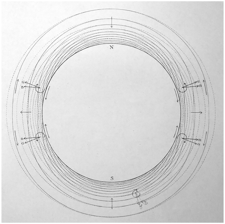
Bjerknes’ vortex theorem applied to the “world medium” atmosphere: isobars (dotted lines) and isosters (solid lines) cross each other and thereby trigger the development of rotary motion (credit: Bjerknes, 1898).

However, from the outset, Bjerknes admitted that the intricacies of actual atmospheric dynamics are much more complex as atmospheric motion is the result of interactions on all of these different scales. In a sense his 1904 paper is also an acknowledgment of this, being a creed of a physicist-by-heart that a completely “rational” treatment of the moving atmosphere cannot just map and count solenoids but must eventually start from the fundamental equations of fluid motion itself, that is, the primitive equations in the tradition of Eulerian fluid mechanics. Thus, neither graphical solutions to cyclone formation nor a cyclone pattern as simulated by a model globe of the atmosphere would ultimately be sufficient. What the Euler equations offer, or symbolically perform, instead, is the iterative treatment of infinitely small parcels of air in infinitely small time steps.

Everything flows (in closed vessels)

When studying the early history of atmospheric modeling in depth, it turns out that the Bjerknes story summarized above might not just be a nice little anecdote to the prehistory of GCMs—the phoenix of weather and climate modeling rising from the ashes of the aether. Instead, it is emblematic of a more fundamental scientific as well as practical relationship between moving and changing air currents and the electric currents that represent it. There is a long-standing, astoundingly close and quite productive mutual reciprocity—in terms of experimental analogies, ontological affinities and epistemic frictions—between the hydrodynamics of the atmosphere and electrodynamics, or, more generally speaking between knowledge about air and its movement and knowledge about electricity and magnetism.

As we experience and conceptualize our global environment today by way of digital representations, as a “mediated planet” (Wickberg et al., 2024) increasingly operationalized and managed through instrumental data and model code, it would be a mistake to think, that this intimate coupling between earthly spheres and electrical media just simply emerged with the dawn of digital computing. In case of the atmosphere, at least, it seems rather grounded in long epistemic traditions in which the fluid envelope of air and electricity/electromagnetism were treated as occupying very similar epistemic terrain, sometimes even as ontological twins, sometimes as antagonists, but always in direct conversation with each other. Now and then this reciprocity found its expression in rather surprising revelations as in the case of Bjerknes tank experiments where one misleading conceptual framework of “hydroelectric forces” entirely fails, only to become paradigmatic for the hydrodynamic treatment of the atmosphere, which will then eventually become only solvable with tiny electric charges, again. These up- and downswings are symptomatic for a longer history of the co-productive episteme of electromagnetism and atmospheric, or, more generally, geophysical fluid dynamics.

It wasn’t just an accidental decision when in 1946 John von Neumann and the Swedish-American meteorologist and student of Bjerknes Carl-Gustaf Rossby decided to launch two projects in direct conjunction, well, literally treat them as one: the (hardware) development of an experimental electronic computer and the (software) development for numerical weather prediction and general circulation modeling. It was just another, albeit extremely momentous turn in the materialization of a mutual epistemic relationship that was already going on for centuries in different technical constellations and with differing possibilities and imaginaries.

Natural philosophers of the 18th century, for instance, were obsessed with flows and circulations—witnessed as much in the rise of fluid dynamics as in the marveled study of the electrical medium. During the first half of the century the new field of hydrodynamics was created out of the material field of hydraulics, decidedly a science of one-dimensional flow in water pipes and tubes. This is particularly evident in the eponymous “Hydrodynamica” by the Swiss mathematician and physicist Daniel Bernoulli as well as his father Johann Bernoulli’s work presented in the “Hydraulica” (Bernoulli, 1738, 1742). Leonhard Euler, who helped his mentor Johann Bernoulli to clarify his mathematics, then devised the symbolic tools, and with them the basic equations, for treating fluids with analytical mechanics—the very Euler equations on which Vilhelm Bjerknes’ programmatic outline and today’s climate models build upon.

Euler’s specific form of calculus, partial differential equations, were indeed first applied in a study by Jean-Baptiste le Rond d’Alembert that responded to a competition arranged by Euler himself and that dealt with nothing other than the general circulation: “Determine the laws that the wind would have to follow if the earth were completely covered by an ocean, so that the direction and speed of the wind could be determined at any time and any place” (d’Alembert, 1747, author’s translation). Although d’Alembert’s submission won the first prize, his pure abstraction remained entirely inapt for the study of atmospheric movement. It neither referred to a meteorological-empirical real world nor was it adequate in its physical approximation. It was, nevertheless, of momentous importance how partial differential calculus and wind dynamics were genetically intertwined for the first time here.

Meanwhile, static electrical phenomena, generated via the “exciting” of rotating glass tubes with ropes, were understood, akin to hydraulic pipes, as “lines of communication,” and constituted a tremendous matter of attention in mid-century natural philosophy (Heilbron, 1979). Euler, together with his son Johan Albrecht, was very keen on explaining the cause of the electric “effluvium,” making use of instruments such as the barometer and concepts such as the aether (Euler, 1759). The whole inspiration for Carl Anton Bjerknes’ water tank experiments, in fact, stems from his readings of Euler’s Letters to a German Princess [dated 1760–1762] which stated that “electricity is nothing else than a perturbation of the aether’s equilibrium” in the form of shakings or vibrations (Euler, 1847: 20). Atmospheric movement, electrical phenomena and the aether created an extremely vibrant triad in 18th century enlightenment, a recombinatorics of varied fluidal theories of electricity, theories on atmospheric electricity, and vortex theories about the aether.

This conceptual blending hardly faded. With regard to electricity in the first half of the 19th century, art and science historian John Tresch speaks of a still ongoing “fluid imaginary: a reservoir of notions which melded with troubling ease from one into another, whose distinctions, intersections, metaphysical bases, and ontological statuses were extremely difficult to pin down” (Tresch, 2006: 62). During the entire warm-up period of modernity, the cross-references between visible and invisible fluids, ponderable and imponderable fluids, real and unreal fluids defined the scientific artistry. Oceanic liquids and airy gases, the aether, electricity, magnetism, light, heat, caloric and nervous fluids, all referred to, or represented, media of the elemental order.

That, of course, could also be said for all historical times, in a sense. Heraclitus’ dictum of the panta rhei (“everything flows”) is a constant in Eastern and Western thought and surely not even confined to that of the Global North. What does a closer look at the changing contact and friction surfaces in between these two (alleged) fluids, the air and electricity, then reveal? Due to its open ontological status Tresch identifies electromagnetism’s role in the first decades of the 19th century as the indetermined other of the mechanistic worldview, a worldview that is epitomized by the French polymath Pierre-Simon Laplace.

Yet, as we go on in time, electromagnetism also becomes the attractor for all those who seek a more thorough fluid-mechanical foundation of physics. Michael Faraday’s 1831 discovery of induction—the creation of an electric current through a changing magnetic field—had made clear that the hydro analogy was not as simple as previously assumed. Still, the new paradigm of the electrodynamic field did not supersede the flow trope but merely served as a specification, which eventually led Vilhelm Bjerknes and the whole of meteorological and oceanographic theory to speak of, and calculate, “flow fields” when dealing with the motion of the two world media. The creator of the fundamental field equations himself, James Clerk Maxwell, imagined Faraday’s lines of force as “fine tubes of variable section carrying an incompressible fluid” (Maxwell, 1855/56: 158) and developed a hydrodynamic and an explicitly vortex-based model to account for the forces occurring in electrophysical space (Maxwell, 1861). In close exchange with George Gabriel Stokes (one of the two physicists behind the Navier-Stokes equations), William Thomson regarded hydrodynamic theory as the principle model for all natural phenomena and especially electrical currents as they were starting to flow through submarine telegraph cables, or actual “lines of communication,” hundreds of miles long (Thomson, 1855). From the opposite end, the actual fluids themselves, Hermann Helmholtz in his seminal paper on vortex motion noticed a “remarkable analogy of the vortical motions of water with the electromagnetic effects of electric currents” (Helmholtz, 1858: 27). Hertz, who set out to create a new foundation for mechanics based on electromagnetism, also entertained a keen interest in meteorological processes in the air, the flow of snow and even the energy balance of the entire Earth (Hertz, 1884; Mulligan and Hertz, 1997). The experiments of the two Bjerknesses were not marginal attempts of scientific outsiders but were in tune with the findings, attempts and common perplexities of the European scientific elite.

Electrotechnical engineering and the creation of the modern world followed along. Historian of technology David Gugerli, who has studied the sociotechnical assemblage created through the electricification of Switzerland—the very Switzerland of the Bernoullis and Euler—, sees a “structural and conceptual attachment of electrotechnical practice to the wealth of hydrodynamic experience” in which the “metaphor of flow . . . became the topos of the discourse about electricity par excellence” in the late 19th and early 20th centuries (Gugerli, 1996: 158 and 174). Even then, on the verge of the electronic age, reified in the radio tube of Hertzian manner that controlled the flow of electrons in order to modulate electromagnetic waves, and after a whole century of standardization efforts of electrical units and equipment, electricity was still something that seemed best addressed through fluid analogies. In 1908 Adolf Slaby, a radio pioneer and first professor of electrical engineering at the Royal Technical Academy of Berlin, wrote in his book on the “Voyages of Discovery Through the Electrical Ocean”:

What happens inside the wire? We do not know. The nature of the electric current, for that is what we call the process, leads the researcher to the limits of knowledge. But where knowledge fails, the poetic imagination guides us: we think of a real flow of the electrical property, similar to the flow of a liquid through a narrow tube. (Slaby, 1908, 32f, author’s translation)

Then, in the 1930s, first attempts were made to arrange and connect electron tubes in such a way that binary numbers could be represented and stored by them (Ceruzzi, 1990). Crucially, this new application was based on the repurposing of components from radio technology for the purpose of radar, where continuous, that is, analog, electromagnetic waves had to be converted into high-frequency digital pulses. These controlled pulses of electron currents now opened up a whole new domain of scientific investigation: that of calculation at (nearly) the speed of light. It would take another twenty years or so before computing went fully digital and the fusion of the IAS Electronic Computer Project with the Meteorology Project was one of the main catalysts of that trend. From then on, the future path for the study of natural system processes through the automated processing of binary signifiers was just a matter of when and how, and much less of an if (Akera, 2006). The shared legacy of electrical and hydrodynamic flow as it was spelled out in myriad ways during the 18th and 19th centuries had finally merged in an epistemic architecture that controlled the flow of electrons in order to represent the flow of ephemeral geofluids.

From the water pipes of the Bernoullis to the glass tubes that emanated a mysterious “electric fluid,” from Maxwell’s imagination of force carrying fluids in fine tubes to the paper tubes of Bjerknes, and then on, finally, to the memory and switching tubes in the IAS machine and elsewhere: Closed, cylindrical vessels constituted the conceptual and material environments in which the natural environment, wide open and unruly, became amenable for calculation. Drawn or engineered enclosures fused together the production of physical laws and symbolic operativity, opening up the possibility of making quantified statements about that very outside world from which they were isolated. Whether the “gurges” (whirls) of water at pipe junctions of different diameter that prompted Johann Bernoulli to treat real fluids analytically (Szabó, 1977: 173), the tube-shaped solenoids of denser and less denser air of Vilhelm Bjerknes, or the “rain of electrons” that the developer of the Selectron tube Jan Rajchman tried to harness for locking information (quoted in Magoun, 2015: 1430), flows and currents became something that was not only studied in either gas-filled or evacuated glassy containers. They eventually also became something to be operationalized inside these very material components (see Figure 5).

Figure 5.

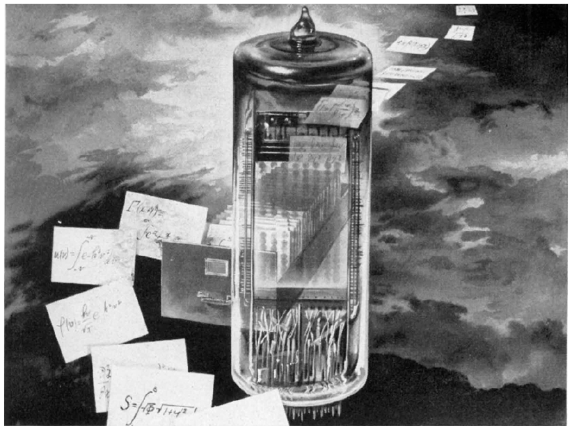
Ad for the “Selectron” tube developed by the Radio Corporation of America (RCA) from 1950. This memory tube was originally intended for use in the IAS machine to aid in weather forecasting (credit: David Sarnoff Library, via Alexander Magoun).

The study aspect is the main reason for creating analog scale models such as the model atmosphere globe of Carl Anton Bjerknes, but also the dishpan models that have a history of their own and were still in high use during the early days of numerical weather prediction. But even here their merit lies more in an illustrative or pedagogical function, than in actual quantification. The second aspect, the operationalization, however, takes place where the steering, switching, amplifying, rectifying, and modulating of electron flows performs no less than the manipulation of the very symbols that since Eulerian times have become to constitute the knowledge about flows of air: in digital and binary electronics. ⁵ With that epistemo-technical transgression, “the world is no longer a function of the subject of perception and its codes, but a function of electronic signal processing” (Siegert, 2003; 391, author’s translation). With the invention of the transistor and the development of solid-state electronics in the 1950s, the elemental, fluidal aspect of this very signal processing became less obvious. But by then, the conceptual leap of binary computing with electronic means was already set in motion. It gradually established its own megastructure of information flow now encircling, monitoring and modeling the globe as a form of planetary computation—with all its fundamental ramifications for transforming this very planet (and the humanity inhabiting it) materially, politically, and conceptionally (Bratton, 2016; Gabrys, 2016; Wickberg et al., 2024).

Blended into each other in the realm of unpredictability

Today, no proper Earth or Earth system science is even thinkable without the electronic treatment of the varied geofluids that flow in, on, and around the globe. Even the convection processes that take place in the Earth’s liquid outer core and generate the Earth’s magnetic field are now simulated by numerically integrating the Euler or Navier-Stokes equations. After all, the Earth itself is nothing other than a magnetohydrodynamic dynamo—the whole reason, by the way, that our planet enjoys keeping an atmosphere and hydrosphere in its bounds. Without this geodynamo the life-giving geofluids would be gone. And while it is susceptible to the same physical forces and mathematical laws (i.e. the deflecting Coriolis force) as is the general circulation of the atmosphere and oceans its turbulent behavior is simulated with the same kind of heuristic and approximative numerics.

I write approximative because that is what all fluids—whether real, ideal, electric, inductive, or imaginary—have in common: their actual behavior is, as a matter of principle, unpredictable. The sudden emergence of vortexes and turbulences, that Bjerknes was carving out with his given symbolic means, is also their most prominent feature. Baroclinity, and thereby instability, is everywhere.

Bjerknes’ crucial theorizing and operationalizing of the atmospheric conditions that lead to vortex generation are hinting at the central importance of instability for the study of the atmosphere and geophysical fluid dynamics more generally. Fluids quite traditionally occupy the domain of the indeterminate and chaotic and it is in this regard that all the attempts and, indeed, successes, of harnessing them with continuum mechanics ought to be understood. It was while playing around with atmospheric GCMs that the meteorologist and mathematician Edward Lorenz discovered, and tried to make a sense of, the stark differences in numerical results when initial conditions only slightly differed—the beginning of what came to be known as chaos theory (Lorenz, 1963). Even physical systems that are principally deterministic can be unpredictable and their behavior not reproduced. The mechanics of flowing air is a prime example of such a system. Atmospheric dynamics cannot be captured by some cog wheel mechanics as it is subject to non-linear interaction across all scales. Sudden changes from laminar to turbulent and back to laminar flow occur without even having a chance to predict or even locate these changes exactly. Every movement is both the effect and cause of every other movement. Regularities are only snapshots of irregularities. In the 1980s Catherine Nicolis, the grande dame of research into non-linear behavior in meteorology and climate dynamics, summarized “the fundamental instability of the atmospheric system” with these words: “a perturbation arising from an uncontrollable localized event and acting on a larger scale phenomenon pertaining to atmospheric circulation may give rise to an (exponentially) divergent history and to an altogether different regime, or to an aperiodic sequence of regimes perceived by an unaware observer as ‘noise’” (Nicolis and Nicolis, 1986).

What Nicolis described, however, did not diverge in principle from insights made much earlier. Virtually everyone, who has ever seriously engaged in “mechanical” readings of the wind—either in physical or philosophical form—knows the fact by heart, that the atmosphere is likely the most eminent realm of instability and unpredictability. The concept of “noise” is not an invention of the present but only its current and especially signal-technical paraphrase of an ancient way of explaining nature. To some extent, the ancient origins of the word chaos highlights that:

“The boundless and all-mixed, the undivided and formless are of oldest tradition. . . . In chaos, the elements are not able to develop their qualities, i.e. they are only potential. This apprehension is scientific. The warm and the cold, the moist and the dry (the four Aristotelian qualities), the soft and hard, the heavy and weightless cannot give the elements their boundaries, their ‘forms’ and ‘realms’, because they are in constant conflict without peace” (Böhme and Böhme, 1996: 41, author’s translation)

Only through divine creation is this chaos pacified and world order created through the differentiation of weightless aether sphere, dry and vaporous air sphere, humid water sphere and heavy earth sphere. However, even after that intervention does the wind remain a phenomenon very “close to chaos” (Böhme and Böhme, 1996: 44), albeit somewhat structured by its allocation to cardinal directions and origins. It is difficult not to recognize some analogical understandings of the problem of atmospheric motion between ancient cosmogony and modern geophysics. ⁶

James Fleming attests Vilhelm Bjerknes a neo-Laplacian agenda when the latter formulated his theoretical program of founding the science of meteorology on mechanical principles (Fleming, 2016: 9, 25, 225f). But also Bjerknes, as Fleming rushes to point out, knew that his set of equations can only point to mere heuristics, and speaks only of “sufficiently accurate” knowledge of the state of the atmosphere at a given time to calculate its future state and a “sufficiently accurate” knowledge of the laws governing the evolution of this system (Fleming, 2016: 25). And even Laplace himself knew it too. One of the most cited references in the history of physical thought is the famous passage of the Essai sur les probabilités where Pierre-Simon Laplace introduces his demon that forever will personify the deterministic world view epitomized in late enlightenment physics. But no one cites the paragraph in the Exposition du systeme du monde from 1796, in which Laplace has immense doubts on the success of such a demon when acting on the other “celestial mechanics,” namely, the sublunar sky, if I may speak a bit anachronistic in Aristotelian terms here. In a chapter specifically dedicated to the “Oscillations of the Atmosphere” he ends with the following clause:

“If we consider all the causes which derange the equilibrium of the atmosphere, its great mobility arising from its elasticity and mobility, the influence of heat and cold on its elasticity, the immense quantity of vapours with which it is alternately charged and unloaded, finally, the changes which the rotation of the earth produces in the relative velocity of its molecules, from this alone that they are displaced in the direction of the meridians, we will not be astonished at the variety of its motions, which will be extremely difficult to subject to certain laws.” (Laplace, 1830, Book IV, 180f)

It seems paradoxical, after all, that electricity, the antagonist of the Laplacian demon, should finally become the operating space on which all of today’s heuristic tools, which try to approximate a solution to this very complexity, are based.

But it’s not. During the heydays of classical mechanics, Laplace speaks of the problems to treat “elastic” systems, “alternately charged and unloaded,” that are not in “equilibrium.” During the heydays of electrodynamics, Vilhelm Bjerknes started to epistemically penetrate the unpredictable behavior of the atmosphere through concepts such as the “field” and metaphors such as “solenoids.” During the heydays of chaos theory Catherine Nicolis’ described the same in terms of dynamical systems theory (“regimes”) and signaling theory (“noise”). These three are just different epistemological and technical ways of framing what is essentially the same problem.

Since the mid-20th century, computer models such as GCMs became highly productive environments to probe chaotic physical realities through numerical experiments. It is somewhat of a truism that such models are reductionistic and therefore embodiments of uncertainty. In fact, that is their very design principle, even down to their innermost core, as has been explained above. Because of their flexibility, numerical models make the unpredictability and instability of the real world available for analytical treatment (Rosol, 2017). But they do so only under the rules organized by binary symbol manipulations within the controlled environments of electron flows and electron storage. These electronic environments impose quite material constraints on any calculation, so that truncations, parameterizations, and strategies of informed guessing determine the operating space for narrowing down and inventing new what-if scenarios, which is what simulations are, in the end. In this way, in-silico experimentation keeps knowledge about earthly processes in a kind of eternal suspense, a perpetual game of binary signifiers in which certainty can never be achieved, but in which speculation is confronted with plausibility checks and new avenues of investigation are opened.

Given this material basis of atmospheric, hydrographic or even comprehensive Earth system simulations, it seems logical and consistent, that although their computer code performs calculations based on mathematical formulas, the entire conceptual approach to these systems is built upon and expressed in electrical engineering terms. Whereas the “fluid imaginary” has played a crucial role in the historical formation of electronics and its epistemic bond to treating actual fluid dynamics until the 1950s, the realm of signal processing has since become the dominant epistemic trope, especially in everything affected by system dynamics. When current Earth system science speaks of the “noisy” flows of airs, or the anthropogenic “signals” to be detected in climate series, or the positive “feedbacks” to be avoided, they literally exhibit an epistemic framework, in which terrestrial processes are cast as processes going on in integrated circuits. This new representation, however, is one that still has ample connections to the world of fluid dynamics and turbulence. Resting on long-standing epistemic traditions, digital binary modeling has only just begun to learn how the flow of tiniest currents resonates with a world of flow.