International climate targets are achievable,but only in models,not in the real world

Abstract

The article argues that the relationships and historical trends of global temperatures and of fossil-fuel production are now both clear and relatively stable. Hence archival data of past performance allow a ‘speedometer reading’ of current rates of change and enable a direct ‘reality check’ on claims about future climate change. Embedded in a new Hubbert-style resource model the historical rates forecast that surface temperatures remain on course to rise by 4.5°C (6°C over land) by the early 2100s. This unsettling prospect is in close accord with several middle-of-the-road projections in the recent sixth IPCC Assessment Report (2021). Instead, if hoped-for targets of carbon neutrality are to be met and global temperature rises held to well below 2°C, as stipulated in the Paris Agreement, then the current rate of deployment of clean power sources would need to accelerate by an unprecedented 100-fold, to around 50 EJ year⁻¹, within the decade.

Introduction

This article steps back from complex computer models of future climate change and instead considers what temperatures are predicted by a largely data-driven approach. It draws on historical time-series (of global temperature and energy use), augmented, where necessary, by insights from atmospheric-chemistry models and compact Earth-system models.

The work focuses on the conundrum that, for climate scientists, recent improvements in the signal-to-noise ratio of the monitoring of global temperatures has led to an increased clarity and to a growing recognition that urgent concrete actions from governments are needed, not distant targets. In contrast, for politicians, the slowdown of the global economy in the wake of the 2008 financial crisis has led to lower fossil-fuel emissions than previously projected and created an excuse to row back on promises made to meet the net-zero commitments of the Paris Agreement.

The decision at stake is whether humanity should focus so strongly on reducing the atmospheric CO₂ content, by reining in global carbon emissions or by capturing the CO₂ already emitted, in order to achieve ultra-low but extremely expensive temperature-rise targets (such as 1.5 or 2°C); or rather we should accept that climate change is coming and instead aim for an economic optimum, a goal long advocated by the 2018 Nobel prize winner William Nordhaus. The ambition would be to achieve environmental goals and to remain within a safe operating space, but at a reasonable cost, and so maximise the wellbeing of the global population. Immediate progress towards meeting this alternative challenge could be the deployment of a smart carbon tax (a progressive tax involving a recycling of tax revenues to refund low carbon consumption). If communicated carefully to the public a well-designed, revenue-neutral carbon tax would promote a judicious balance between adaptation and mitigation measures through a consideration of costs and damages avoided and/or benefits gained (Nordhaus, 1977; Pigou, 1920; Thompson, 2017).

Earlier critiques that have been raised before about fossil-fuel availabilities and the implications of fossil-fuel supply constraints on climate-change projections include Doose (2004), Kharecha and Hansen (2008) and Wang et al. (2017). Also Lean and Rind (2009), as an alternative approach to using numerical model simulations to assess climate change, employed a direct analysis of surface temperature observations. By quantifying specific changes arising from natural and anthropogenic influences Lean and Rind were able to use their empirical approach, anchored in the reality of observed changes in the recent past, to forecast surface warming over the next two decades. What is new here is a climate prediction calibrated directly using the relationship between historical fossil-fuel use and the global temperature rise and so able to generate a forecast of surface warming many decades ahead. The new, reduced-order model has few important terms, is of low complexity and only modest input from other integrated assessment models (IAMs). This is helpful as IAMs are generally based on a multitude of assumptions involving often-intricate linkages between the principal features of society and economy (population increase, future development, economic growth, land use, food security, energy provision) with the physical processes of the biosphere and atmosphere. On the other hand, the leading variables of the reduced-order model can be evaluated directly from the primary (historical) data bases of global temperatures (Table 1 & Figure 1) and energy-use and emissions (Table 1 & Figure 2). In this way, by using empirical, real-world evidence, the vexed question of how to derive a precise climate sensitivity from climate models is nullified. In short, by simplifying the climate-change problem to its essentials, the reduced-order modelling offers the prospect for a greater understanding of the baseline, practical fundamentals of the conundrum that is climate change, and especially for creating a greater awareness of the necessity for prompt action.

Table 1.

Four key variables.

Variable a	Symbol	Value	Source
Warming to now	ΔT now	1.3°C	Berkeley Earth
Years to peak ff production b	tff	20 years	Mohr et al. (2015)
Warming rate to ff peak	δT/δt	0.03°C/year	Cheng et al. (2022), Berkeley Earth
Reserves at peak	Rff	0.6 Skew = 1+ 0.6/(1–0.6) =2.5	Dittmar (2016, 2017), Höök et al. (2009, 2010, 2014)

a

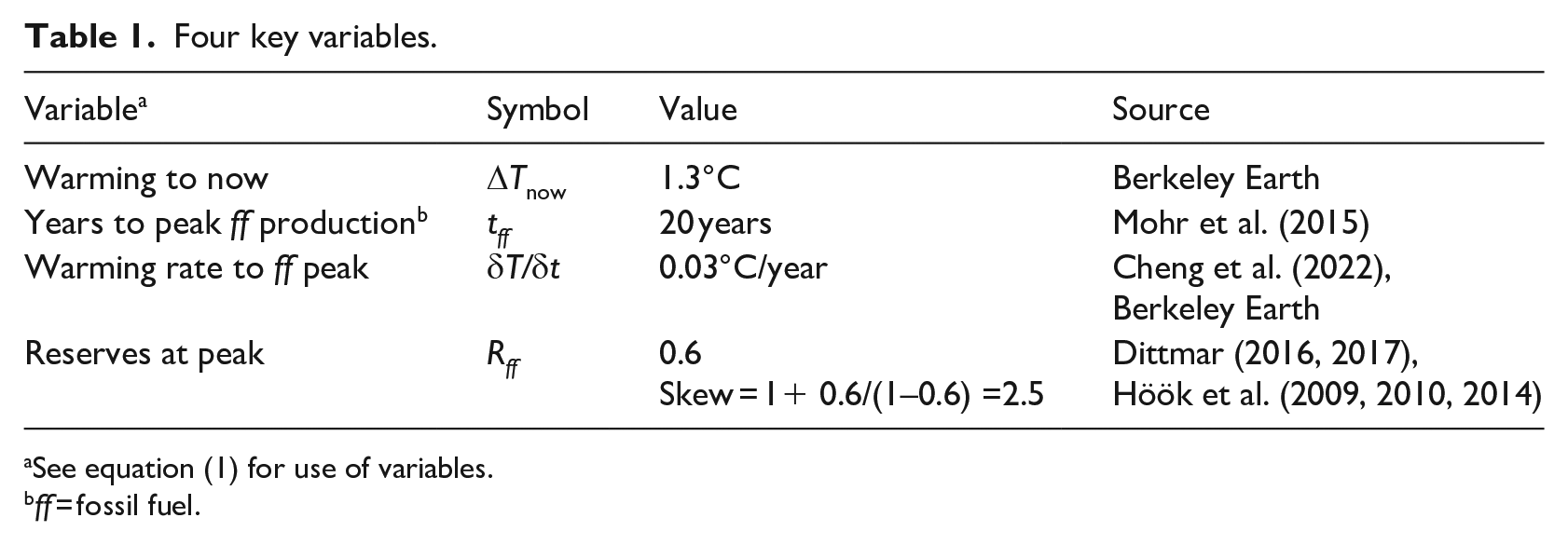
See equation (1) for use of variables.

b

ff = fossil fuel.

Figure 1.

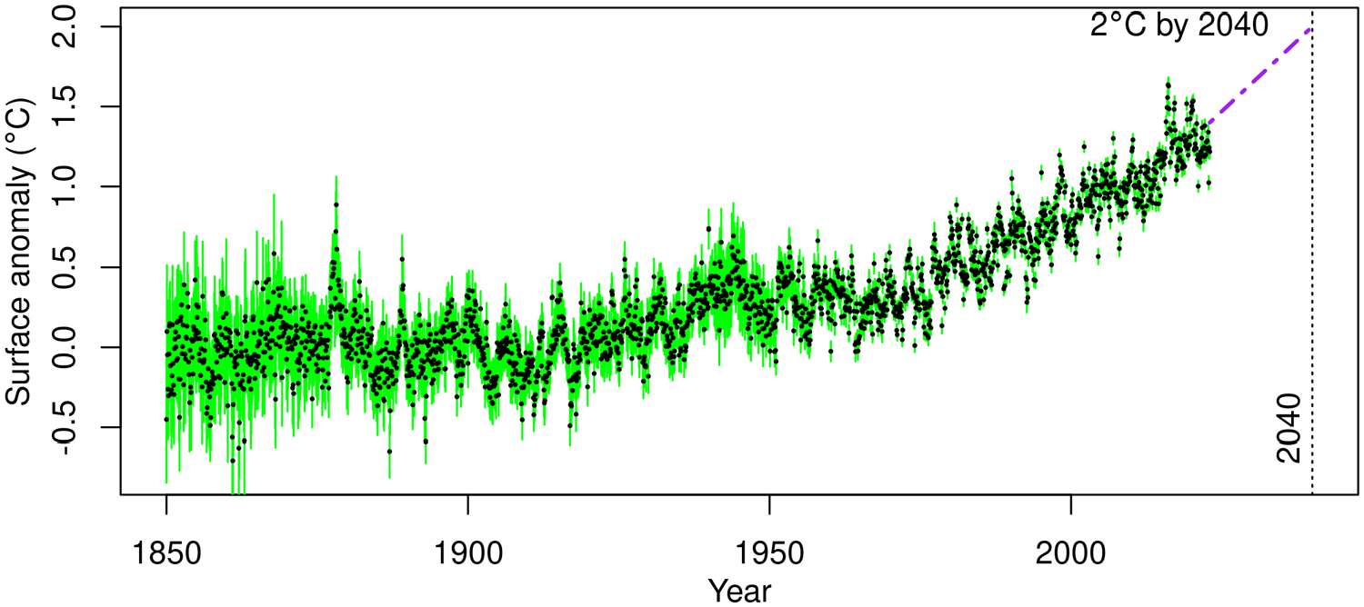
Average global surface temperature anomalies (black dots) and uncertainties (green bars) for each month since 1850. Temperature anomalies plotted with reference to an 1850–1900 baseline. (The reference period 1850–1900 is commonly used to represent pre-industrial temperature.) Purple dash-dotted line forward projection to 2040.

Figure 2.

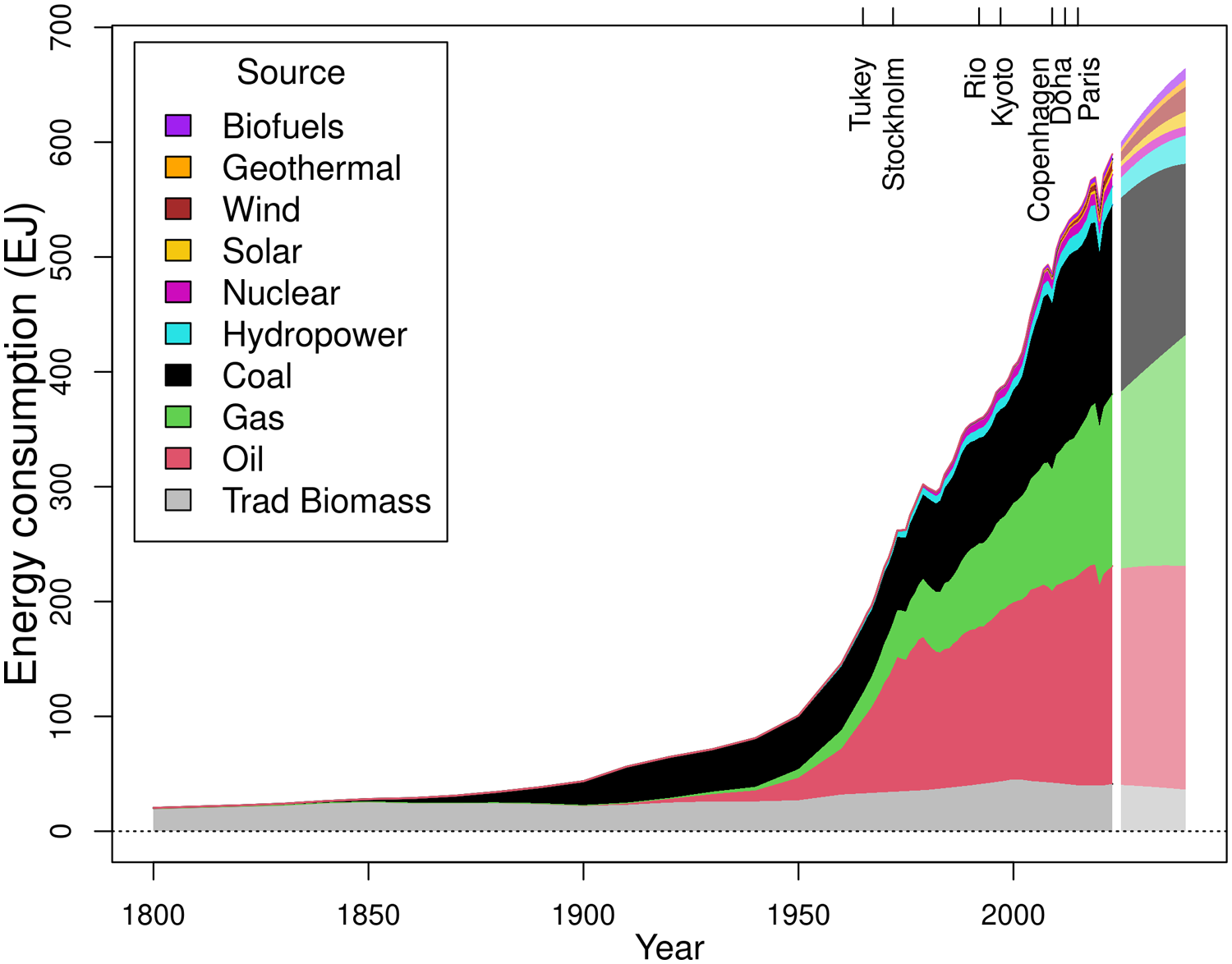
Global energy consumption (in units of Exajoules) for 10 energy sources, each year from 1800 to 2022 and projected forwards for the years 2023–2040. Tick marks (top axis) mark dates of major international meetings that highlighted concerns over impending climate change. Despite such warnings fossil fuels are seen to have continued in their dominance and their emission rates to have doubled. Curves to the right of the white vertical stripe are forward projections based on the long term trends over recent decades.

The world remains highly dependent on fossil fuels. Global energy consumption has been increasing markedly ever since the 1950s. Although the percentage share of renewables has been growing, it has not been able to keep up with the gross rate of expansion of global energy consumption. The energy shortfall continues to be met predominantly by an increasing reliance on fossil fuels. Consequently, coordinated global action with proper carbon pricing (which embeds the ‘social cost’ of carbon dioxide in the wholesale cost of fossil-fuels) remains an imperative for ameliorating anthropogenically induced warming and forestalling strongly rising sea-levels (Hansen et al., 2022).

This article closes by briefly reflecting on which specific predictor variables, in the new data-driven, reduced-order-modelling approach, are the most important, or the most influential, and which are the most poorly constrained. Uncertainties and confidence limits are notoriously large in climate-change studies and more uncertain than is often assumed by policymakers. One advantage of the data-driven approach is that its transparency, simplicity and understandability can help the investigator grapple directly with conceivable sources of uncertainty.

Empirical evidence

The article contends that time-series of past surface temperatures and global-energy use allow a strong causal relationship to be constructed and expressed mathematically. Moreover, on the assumption that the overall pattern of the relationship will continue into the future, it also asserts that a useful forecast of impending temperature change can be made based on past and present data and by an analysis of trends. The two key, historical time-series required to drive the forecast are past global temperatures (Figure 1) and fossil-fuel use (Figure 2). The information contents of these two time-series are combined using the well-known finding that global mean surface warming is approximately proportional to cumulative (total) CO₂ emissions (Matthews et al., 2009), alongside the premise that the burning of fossil fuels has been the dominant contributor to rising levels of CO₂ and to recent global warming. In essence the underlying mathematics assumes that cumulative carbon emissions, with at most a very short delay (Ricke and Caldeira, 2014), will largely determine global warming levels into the late 21st century and beyond.

Methodology

Expectation of a continuance of long-term rates of change with only gradual adjustment is a crucial element of the article’s energy-based methodology. Energy transitions on the global scale, as Smil (2016) has emphasised, are inherently protracted affairs. He points out how widespread systems with a great degree of reliance on a singular energy source have elaborate, costly and enduring infrastructures. Consequently, substitutions by new energy sources must inherently be of a gradual nature. This unremitting situation is well illustrated by Figure 2, where the continued reliance on fossil-fuel-derived energy is seen to endure (on multi-decadal time scales) despite strong exhortations from international climate conferences (Stockholm, Rio de Janeiro, Kyoto, Copenhagen, Doha, Paris) stretching back over half a century to 1972, and to the even earlier specific warning of the President’s Science Advisory Committee Report on Atmospheric Carbon Dioxide (Tukey, 1965: 112–131). Throughout these decades, predictions of imminent technological triumphs and for accelerated transitions from fossil fuels to renewable energies have remained largely unrealised. These failings are starkly illustrated in Figure 2 by the steadfast narrowness of the stripes for renewables compared to the broad swaths for oil, gas and coal. There is no sign, in Figure 2, of a low-carbon transition having had a substantive impact on a global basis. On the contrary, long-run fossil-fuel use can be seen to be continuing to grow rather than to abate. Indeed, carbon emissions related to global energy provision grew during the last year (2022) to reach a record high. While small falls in energy consumption have occurred (due to the 1970s oil price shock, banking crises of the 1980s and early 1990s, and the COVID-19 pandemic) these have all quickly reversed. The deep-rooted inertia in large-scale energy systems, evident in Figure 2, is a key justification for using applied time-series analysis as a forward-projection technique.

In this article the prediction of future temperatures focuses on the top temperature that will be reached, plausibly sometime in the early 2100s, when humankind’s exploitation of fossil fuels weakens as economically recoverable resources become exhausted. A Hubbert-style resource model (Hubbert, 1956) drives the prediction. The heart of the approach is a straightforward, linear calculation that boils down to scaling up the temperature change, between pre-industrial times and the time of peak fossil-fuel emissions, by the ratio of the fossil-fuel resource recoverable before and after peak production. This basic calculation is easily refined (as shown below) to incorporate second-order anthropogenic effects such as from methane and aerosols emissions in addition to the main driver, CO₂ emissions.

In summary, the methodology employed here takes two different approaches compared to IPCC/CMIP (Intergovernmental Panel on Climate Change/Coupled Model Intercomparison Project): (i) it derives a climate sensitivity from observations, not climate models and (ii) it derives fossil-fuel emissions scenarios from Hubbert-style resource models, not IAMs.

Sources

Global surface temperatures, and their uncertainties, were sourced from Berkeley Earth. Version 1 of their temperature anomalies is used, in which the land component is combined with ocean data from HadSST4 as described in Rohde and Hausfather (2020). Units of °C are used in plotting the time-series in Figure 1.

Global energy data were sourced from Ritchie et al. (2022). The primary sources are Appendix A in Vaclav Smil’s book, Energy Transitions: Global and National Perspectives (2016) and British Petroleum’s (2022) Statistical Review of World Energy. The energy consumption data, for every decade from 1800 to 1960, and then for every year from 1965 to 2022 (Figure 2), are presented in units of EJ (exajoules). The choice of consumption data ensures consistency between the varied fossil and renewable data-sets. The Global Carbon Budget (Friedlingstein et al., 2022) provides equivalent annually updated data for coal, oil and gas but in terms of CO₂ emissions in units of GtC year⁻¹, as described in detail by Andrew and Peters (2021). Electricity produced by nuclear power plants, expressed per capita, taken from NationMaster.

Scenario information about non-CO₂ contributors was taken from Riahi et al. (2017), Thornhill et al. (2021) and the excellent Excel spreadsheets provided alongside Chapter 6 of the Working Group I Contribution to the IPCC Sixth Assessment Report (Blichner and Berntsen, 2023).

Future warming

The main finding of this article is that surface temperatures are on course to rise 4.5°C (6°C over land) by the early 2100s. Such a temperature projection is far removed from the COP27 target of 1.5°C–2°C. The forecasting methodology is explored in more detail below, where a first, basic projection is gradually refined, in three stages, by representing global change in ways that are progressively more accurate and truer to life.

A basic projection

An initial, crude future projection is to simply double the temperature rise that will have taken place when fossil-fuel production peaks (when half the resource has been exploited). By adopting a midpoint reached within a decade or two, when the temperature anomaly based on current trends would be around +2°C, a final rise close to +4°C is generated. Although rudimentary, this simple ‘business-and-politics-as-usual’ approach accords well with past behaviour: that is, total global energy consumption has risen sharply since 1950 (Figure 2) and shows no sign of abating soon; gas and coal production have continued to climb since the 1980s and their long-terms trends only show minor signs of moderating (Figure 2). Only oil is currently levelling off. In point of fact, worldwide CO₂ emissions hit a new record high of 36.6bn tonnes of CO₂ in the current year (2022) according to the Global Carbon Project’s most recent annual data (Friedlingstein et al., 2022).

For this first, uncomplicated projection the underlying assumptions are easily discerned and stated. They are: (i) since 1850, almost all the observed long-term surface warming can be explained by greenhouse gas emissions; (ii) anthropogenically mediated global warming is dominated by the burning of fossil fuels, specifically cumulative (total) CO₂ emissions; (iii) transitions in the global energy system are inherently protracted affairs; and (iv) fossil-fuel production will continue to follow a Hubbert-style symmetrical, bell-shaped pattern.

Justification of the reasonableness of the first assumption increasingly comes from the amazing advances latterly achieved in monitoring temperature change throughout the Earth system, as discussed and enumerated in more detail below. The second assumption is a long-held tenet of the global warming problem. The third, as explained in the methodology section above, is merited on many counts: the major inertia in large-scale industrial supply chains; complex, enduring infrastructures; the ponderous, long-run systemic patterns manifest in Figure 2. The last assumption, of the Hubbert-peak approach, lays the foundation for the basic driver behind the reduced-order model. Hubbertian behaviour is fitting on account of it being a general earth-science phenomenon. In addition to its most widely recognised application to peak oil and peak gas in scores of production areas from all around the world (Appendix B in Campbell, 2005), Hubbertian behaviour is found to apply in many other geological situations. Historically, since 1815, production of German, Japanese and UK coal (Höök et al., 2010) and of Pennsylvanian anthracite (Höök and Aleklett, 2009) have all steadfastly followed Hubbertian patterns through to their exhaustion. Non-fuel utilisation of Hubbert’s methodology includes the output from all the world’s gold mines, the production peak in antimony and the mining of numerous other mineral commodities such as lithium.

The skew factor

A first refinement of the basic projection is to relax the assumption of symmetry. This helps because, since Hubbert’s (1956) pioneering studies, past-production curves of giant, longer-lasting oil and gas fields have been found to be asymmetrical. Commonly more production takes place post-peak. Many geotechnical examples of skewed field behaviour, from all around the world, are given in the compilations of Dittmar (2016, 2017) and of Höök et al. (2009, 2010, 2014). Typically 60% of the exploitable fossil-fuel reserves remain at the time of peak production (see especially Figures 6 and 9 in Höök et al. (2014), also Figure 5 in Mohr et al. (2015). This level of depletion gives rise to the multiplier (skew factor) of 2.5 tabulated in Table 1 and incorporated into equation (1) as follows:

$$\mathrm{Temperature}\mathrm{change}\mathrm{by}\mathrm{early}2100\mathrm{s}=\mathrm{\Delta }T\prime \times \mathrm{Skew}$$

(1)

where ΔT′ = global temperature rise since the pre-industrial (= ΔT_now + t_ff × δT/δt_decadal); the single prime indicates the temperature response at the time of peak fossil-fuel production; and the Skew factor describes the asymmetry in fossil-fuel production: Skew = 1 + (R_ff /(1 − R_ff)), with R_ff being the exploitable fossil-fuel reserves remaining at the time of peak production (expressed as a proportion of the ultimate recoverable resource). [See Table 1 for values adopted for all variables.]

Land amplification factor

A second refinement is to estimate temperatures over land, rather than in terms of a global average. This straightforward addendum uses a well-known climate outcome that as you put more heat into the global climate system the land warms more quickly than the oceans. The ratio of land to ocean warming is known as the ‘amplification factor’. It is a fundamental response in climate-change studies as shown by the same land-ocean warming ratio being found in recent climate observations and in simulations by global circulation models. The temperature contrast arises in part because land has a smaller ‘heat capacity’ than water. But also, local evaporation plays a part: oceans have unlimited water to evaporate, so in a warming climate they can efficiently cool themselves. Wallace and Joshi (2018) derive a land-ocean amplification factor of 1.6, a value adopted here. It translates into a factor, Ϙ^*, of 1.3 when comparing land-only and global-average temperatures.

Aerosols, methane and other non-CO₂ contributors

A final refinement step, used in this article, is to include additional, non-CO₂, emissions of an anthropogenic origin. Over and above CO₂, the next two most important anthropogenic drivers (Gidden et al., 2019; Mahowald et al., 2017) are found to be methane (a greenhouse gas, which warms) and aerosols (which scatter and cool). The latter, to a large extent are associated with sulphur dioxide emissions from burning coal. Global emissions of several other potentially potent components have been growing through the industrial period. These include nitrous oxide, nitrogen oxides, F-gases and volatile organic compounds. Their contributions are many and varied. Several components being greenhouse gases, tend to warm. Whereas SO₂ and NO_x, being the main precursors of anthropogenic sulphate and nitrate aerosol scatterers, cool. Non-CO₂ emissions can exhibit complex chemical behaviours resulting in chemical reactions that affect the greenhouses gases O₃ and CH₄ via atmospheric chemistry and so further modify Earth’s radiative balance (Hoesly et al., 2018). The importance of the non-CO₂ contributors depends on their atmospheric lifetimes, warming potentials, and growth rates (Friedlingstein et al., 2022). So, as is well known, it tends to be their atmospheric concentrations that are of most concern, rather than their cumulative emissions.

What might be the future contribution to climate change from the radiative forcings of non-CO₂ emissions? Unfortunately, there is no simple equivalent to the Hubbert-curve for fossil-fuel production for forecasting changes to these contributors. Instead, a profitable procedure is to consult outputs from atmospheric-chemistry models driven by feasible scenarios (Shared Socioeconomic Pathways, SSPs) of projected economic activities. In this article ‘middle of the road’ scenarios of non-CO₂ emissions, such as SSP2-baseline, SSP4-baseline and SSP4-6.0 are favoured (see IPCC, 2021 and also Pedersen et al., 2021, for SSP acronyms and summaries). A first point of note is that atmospheric-chemistry models indicate that the sum total of non-CO₂ components accounts for 30% of today’s warming (Blichner and Berntsen, 2023; Thornhill et al., 2021). Secondly, turning to future projections, a warming contribution of around 1°C, by the early 2100s, is found for scenarios in which the long-term trends continue: that is, in which air pollution declines, while the concentrations of non-CO2 greenhouse gas (GHG) components gradually increase. The first effect reduces ΔT′_CO2 (the estimated rise from just CO₂) by 30%, whereas in contrast the second effect increases ΔT′′ (the total temperature response in the early 2100s). Briefly, as they are of a broadly similar magnitude the effects largely cancel each other out in equation (2).

Early 2100s

Although coal use rapidly increased as steam power improved throughout the 1800s to become the dominant provider of horsepower for industry (Wrigley, 2013), global use of energy derived from fossil fuels only truly took off in the 1950s (see slope change in Figure 2) when oil and natural gas began to replace coal. Consequently, a peak fossil-fuel consumption, around 2040 (Table 1), would round off a 90-year long period of growth (1950 to 2040). Decline over a comparable (symmetric) 90-year long period would lead to the ultimate demise of fossil fuels in the early 2100s. Equation (2), which incorporates the refinements noted above, provides an estimate of temperature rise at that era:

$$\mathrm{Temperature}\mathrm{rise}\mathrm{over}\mathrm{land}\mathrm{by}\mathrm{early}2100\mathrm{s}={Ϙ}^{*}\times \left[\left(\mathrm{\Delta }{T^{\prime }}_{\mathrm{CO}2}\times \mathrm{Skew}\right)+\mathrm{\Delta }{T^{\prime \prime }}_{\mathrm{Non}-\mathrm{CO}2}\right]$$

(2)

where Ϙ is an amplification factor (the star indicates the use of a land/global factor); the single prime indicates temperature responses at the time of peak fossil-fuel production, and the double prime indicates temperature responses apposite to the early 2100s. NB. the skew factor (see equation (1)) is only applied to the temperature rise at the time of peak fossil-fuel production resulting from CO₂ forcing.

Substituting the values of the variables, enumerated in Tables 1 and 2, into equation (2) yields the main result of this article: the forecast of an average warming over land in the early 2100s of 6 degrees (in the absence of unpredictable calamitous globally disruptive events, or massive scale-up and global deployment of new clean technologies). In the broadest of terms, of the additional 2°C rise over and above the initial (crude) estimate of 4 degrees, the main contribution is from the land amplification factor. Slightly less comes from the asymmetry, while non-CO₂ contributors induce the smallest correction.

Table 2.

Secondary variables.

Secondary variable a	Symbol	Value	Source
Amplification factor	Ϙ	1.6 (ϙ* = 1.3)	Wallace and Joshi (2018)
Contribution to present day warming by non-CO2 components	%	30%	Figure 6.12 in Blichner and Berntsen (2023)
Temperature response in early 2100s by non-CO2 components	ΔT′′Non-CO2	1°C	Meinshausen et al. (2020); middle-of-the-road SSP outputs

a

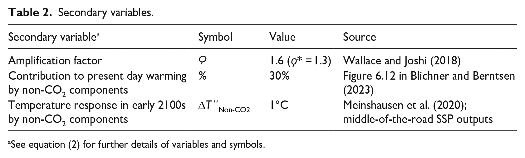
See equation (2) for further details of variables and symbols.

Uncertainties

An elementary sensitivity analysis of the forecast, using a propagation of errors procedure, allows an evaluation of how much each input variable contributes to the output uncertainty. Following a one-at-a-time perturbation approach it is found that of the variables in Tables 1 and 2 the most influential is the post-industrial warming that has taken place to now (ΔT_now). The least influential is the effect of the non-CO₂ components. Intermediate, in consequence, are the number of years remaining to peak fossil-fuel production, the warming rate to peak, and the proportion of reserves at peak. Out of all the key variables the ordering picks out the magnitude of the temperature rise, between the pre-industrial and today, as being the most decisive. Consequently, it testifies to the reconstruction and homogenisation of long instrumental time-series, and to an understanding of the distribution (and redistribution) of heat, both on land and in the oceans, as being a continuing fundamental undertaking in climate-change studies.

Discussion

Other factors

Equation (2) is a simplification and an idealisation. But it is hoped that the features it incorporates are those of greatest importance in the present state of knowledge. Might any additional, vital, anthropogenic sources be missing from equation (2)? Two candidates worthy of consideration are: land-use change and cement manufacture.

Land-use change (especially deforestation) has contributed a sizeable fraction (~28%) of historical CO₂ emissions (Simmons and Matthews, 2016). At first sight this might appear to present a difficulty. Interestingly, however, warming from the CO₂ released during forest conversion to pastoral and agricultural land is found to be offset by a cooling caused by an increased albedo, which allows more incoming solar radiation to be reflected back into space. Indeed, model simulations (Simmons and Matthews, 2016), for both the historical period: 1750–2000, and for scenarios of 21st century change: 2000–2100, show these two competing effects as balancing each other out quite closely, thereby negating any need for their inclusion in equation (2).

The global demand for cement has increased sharply, with a 10-fold increase in global consumption during the last 65 years (Monteiro et al., 2017). The cement industry is currently responsible for approximately 5% of global anthropogenic carbon dioxide emissions (Mahasenan et al., 2003; Mohamad et al., 2022). Furthermore, Mahasenan et al. suggest that if the industry does not improve its specific emission rates, its relative contribution to anthropogenic CO₂ emissions will increase over the next century. So, does cement present a difficulty for equation (2)? Emission scenarios, as typically adopted by IPCC (Nakicenovic et al., 2000), contemplate cement demand as peaking around 2060 or else continuing to increase into the 2100s. Such an outlook bears a close resemblance to the asymmetrical-Hubbert-resource model already used in equation (2). Thus, the trend-driven calculation of equation (2) already largely caters for cement. If any adjustment were judged to be necessary, it would be to marginally increase the temperature forecast, but only by a fraction of one degree.

Assumptions and potential limitations

Turning to the assumptions behind equation (2): a potential limitation relates to the assumption that global warming has been dominated by anthropogenic factors rather than by natural processes. However, this assumption is well vindicated by the amazing strides recently achieved in monitoring temperature change throughout the Earth system – from the ocean depths (Cheng et al., 2017) to its surface, up through the troposphere and stratosphere (Steiner et al., 2020) to the very top of the atmosphere (Loeb et al., 2018). These remarkable new surveillance technologies have allowed the redistribution of heat within the Earth system to be unravelled, tracked, and quantified (von Schuckmann et al., 2020) in great detail. These new systems observe Earth’s additional heat as penetrating ever deeper into the oceans (Trenberth and Cheng, 2022) and not ascending upwards, as might have been anticipated for an internal, unknown naturally driven variability.

A second potential limitation might be that changes to the carbon cycle are not specifically addressed in equation (2). A reasonable question for moderately high fossil-fuel-emission scenarios such as the Hubbert-resource projection used here, is to what degree will natural sinks be able to keep pace with all the CO₂ being released from fossil-fuel burning? Specifically, will the fraction of emissions that remain in the atmosphere increase? Numerical carbon-cycle modelling is a central technique in climate-change work. Such models have evolved, over recent years, into extremely complex tools. They compute CO₂-transfer rates between the main global reservoirs: that is, the atmosphere, biosphere and oceans. The Earth-system modelling work of Liddicoat et al. (2021) addresses the above misgiving. They find (see left-hand panels in their Figure 15) that over the next century the cumulative airborne fraction remains rather steady for moderately high-emission scenarios, such as scenarios SSP4-6.0 and SSP3-7.0 which are not dissimilar to the projection used here. As Liddicoat et al explain a fortuitous steadiness in the cumulative airborne fraction arises when the combined sink strength of CO₂ closely keeps pace with the amount of CO₂ being released. This balance only applies to intermediate emission scenarios, and not to the highest emission scenarios such as SSP5-8.5 (with very high GHG emissions: CO₂ emissions tripling by 2075) nor to lower emission scenarios such as SSP1-1.9 (with very low GHG emissions: CO₂ emissions cut to net zero around 2050). Consequently, the intermediate emission scenario of equation (2), as it stands and as driven by the variables of Tables 1 and 2, needs no additional correction for carbon-cycle effects. In essence the equation carries forward information about the airborne fraction, gleaned from the temperature rise through the historical period, into the coming century.

“imaginary” technological promises

Throughout the history of climate change (especially over the six decades since the Tukey report of 1965) an ever-evolving spectrum of technological and engineering advancements has been put forwards as holding out hope for a rapid and effective solution to the global warming problem. A thoughtful synthesis is provided by McLaren and Markusson (2020) who identify a stepwise, phased sequence from around 1990 to today. Unfortunately, in practice, as McLaren and Markusson set out in detail, and as is evident in Figure 2, carbon emissions have continued to rise rather than stabilise or decline towards net zero. That is, former technological promises have had limited material delivery at the global scale. McLaren and Markusson explain how these ‘imaginary’ technological promises ‘have enabled policy prevarication, leaving [climate] mitigation poorly delivered, yet the technological promises often remain buried in the models used to inform policy’. McLaren and Markusson go on to candidly point out that ‘history reveals that [today’s] contemporary climate engineering promises are nothing unique’. They conclude by describing the five phases (from Rio to Paris: see labels on the top axis of Figure 2) as delineating ‘a series of technological promises whose parameters and capabilities were at least as much “constructed” by models and modellers as by engineers and scientists’. In contrast, the reduced-order modelling pursued here focuses on fewer important terms. As such it is hoped, as it is based on real-world data, that it can contribute to McLaren and Markusson’s rallying cry ‘to encourage more researchers to examine the potential [for the] redrawing of modelling parameters . . . [and the] need for greater reflexivity over the processes by which [climate] targets are reframed, responses assessed, and models deployed’.

Comparison with traditional scenarios

The reduced-order, Hubbertian-led model of equation (2), with fossil-fuel emissions declining after 2040 can be broadly thought of as ‘middle-of-the-road’: that is as falling within the range of intermediate to medium-high emission scenarios. It certainly ranks well below the first IPCC ‘business-as-usual’ (or SA90 Scenario A) model with fossil-fuel emissions growing 2% annually to 2100 (see Pedersen et al., 2021 for performance details of the various families of emission scenarios). It also ranks below the well-known RCP 8.5 scenario, with an emissions pathway characterised by increasing greenhouse gas emissions throughout the 21st century, and even beneath RCP 6 (a stabilisation scenario), with a broad emissions peak centred in the neighbourhood of 2080. The high temperatures forecast by the reduced-order model, instead, emanate from the direct, largely empirically data-driven, calibration of observed temperature rise with fossil-fuel emissions.

Wider implications

As a final discussion point: what may the results presented in the article mean for the general public? The Hubbertian resource-based forecasting approach provides a context to the difficult question: what needs to be done, in terms of power generation, to keep global temperatures low and well below 4.5°C (6°C over land)? In 2021 the contribution of new ‘green’ technologies to global energy was less than 3%. Before the dual short-term shocks of the global COVID-19 pandemic and the Russo-Ukrainian War, their contribution was increasing at a rate of just 0.5 EJ year⁻¹ (Figure 2, using data from BP’s Statistical Review of World Energy). If net-zero targets are to be met, and global temperature rises held to below 2 °C, the rate of deployment of clean power sources will need to accelerate 100-fold, to around 50 EJ year⁻¹, within the decade. One way to visualise the massive task required is by simplifying the energy-resource change required into one of replacing the energy currently provided by fossil fuels with that of a single source, such as solar, or a new generation of nuclear reactors. As an illustration consider the later: currently there are 439 nuclear reactors in operation in 30 countries around the world. These have a combined total output of 10 EJ, almost identical to the total power generation of wind and solar all across the world (Figure 2). If the fossil-fuel problem were to be solved by nuclear reactors alone, 50 EJ of nuclear power would need to be added each year for the next decade (cf. Figure 2). This corresponds to an additional two thousand reactors coming into service each year.

Qvist and Brook (2015, Figure 2 and Table 4) point to the 1970s–1980s as the time of peak deployment of new nuclear power plants when Sweden and France achieved sustained rates of additional nuclear capacity of 600 kWh/year/year/capita (2 GJ/year/year/capita). According to Qvist and Brook a worldwide duplication of this best-case deployment could displace fossil-fuel electricity within 25–34 years. However, when considering the world’s entire energy system (not just electricity generation), and when taking regional economics into account (but leaving aside contemporary problems associated with today’s spectrum of public concerns over plant safety, waste disposal and nuclear terrorism, or difficulties over the levels of investment required), the fossil-fuel displacement timetable extends to over a century. This estimate, of a best-case timescale (~110 years), is obtained by dividing the total fossil-fuel-energy production needing to be displaced (550 × 10¹⁸ J/year, see Figure 2) by the exemplar deployment rate noted above (2 × 10⁹ J/year/year/capita), followed by a scaling up to the richest quarter of the world’s future population (10 billion/4) who might plausibly bear the investment costs. Even this hugely optimistic scenario falls well short of the rapid transition required to achieve carbon neutrality by mid-century if the targets stipulated in the Paris Agreement are to be attained.

Conclusions

Recent, internationally agreed, climate targets are achievable but only in models, not in the real world. Stepping back from complex super-computer modelling an evidence-based, largely data-driven, procedure forecasts a 4.5°C rise in global surface temperatures (+6°C over land) by the early 2100s. The new approach (built around a Hubbert-style resource set-up) boils down to scaling-up observed temperature change, since pre-industrial times, by the proportion of fossil-fuel resource still recoverable. The new procedure has become possible because climate and energy-production records are now so extensive that these historical, globally unified, datasets permit a direct ‘reality check’ on claims about future climate change. A crucial element in the projection is the expectation of a continuance of long-term rates of change caused by deep-rooted inertias in the world’s overall energy system. Five key features are found to determine how far future temperatures will rise: how much fossil-fuel remains to be burnt, the temperature when fossil-fuel production peaks, a land amplification factor, aerosols, and methane.

A global transition to sustainable energy is under way, but it has barely begun. Today (2022) energy production from new, renewable sources (biofuels, wind, solar) makes up only 3% of global energy use, compared to 85% for fossil fuels. Indeed, worldwide CO₂ emissions from fossil-fuel combustion and industrial processes hit a new all-time high of over 36.8bn tonnes of CO₂ in the current year. Disturbingly, global temperatures have already surpassed 1.3°C above preindustrial and are set to reach + 2°C by 2040.

If net-zero targets are to be met, and global temperature rises held to below 2°C, current rates of deployment of clean power sources will need to accelerate by an unprecedented 100-fold. Smart carbon pricing (built around a progressive, refundable tax) offers the best way to provoke a rapid breakthrough and steer global economies and technologies towards the most advantageous future possible. Economists have long advocated Pigouvian-based carbon pricing as the best way to bring about a speedy energy transition: by sending a powerful price signal and by harnessing the invisible hand of the marketplace as a means of determining the most efficient (or lowest cost) approaches to slowing greenhouse gas emissions, thereby fostering a low-carbon future.