The Searsville Lake Site (California,USA) as a candidate Global boundary Stratotype Section and Point for the Anthropocene series

Abstract

Cores from Searsville Lake within Stanford University’s Jasper Ridge Biological Preserve, California, USA, are examined to identify a potential GSSP for the Anthropocene: core JRBP2018-VC01B (944.5 cm-long) and tightly correlated JRBP2018-VC01A (852.5 cm-long). Spanning from 1900 CE ± 3 years to 2018 CE, a secure chronology resolved to the sub-annual level allows detailed exploration of the Holocene-Anthropocene transition. We identify the primary GSSP marker as first appearance of ^239,240Pu (372–374 cm) in JRBP2018-VC01B and designate the GSSP depth as the distinct boundary between wet and dry season at 366 cm (6 cm above the first sample containing ^239,240Pu) and corresponding to October-December 1948 CE. This is consistent with a lag of 1–2 years between ejection of ^239,240Pu into the atmosphere and deposition. Auxiliary markers include: first appearance of ¹³⁷Cs in 1958; late 20th-century decreases in δ¹⁵N; late 20th-century elevation in SCPs, Hg, Pb, and other heavy metals; and changes in abundance and presence of ostracod, algae, rotifer and protozoan microfossils. Fossil pollen document anthropogenic landscape changes related to logging and agriculture. As part of a major university, the Searsville site has long been used for research and education, serves users locally to internationally, and is protected yet accessible for future studies and communication about the Anthropocene.

Plain Word Summary

The Global boundary Stratotype Section and Point (GSSP) for the proposed Anthropocene Series/Epoch is suggested to lie in sediments accumulated over the last ~120 years in Searsville Lake, Woodside, California, USA. The site fulfills all of the ideal criteria for defining and placing a GSSP. In addition, the Searsville site is particularly appropriate to mark the onset of the Anthropocene, because it was anthropogenic activities–the damming of a watershed–that created a geologic record that now preserves the very signals that can be used to recognize the Anthropocene worldwide.

Introduction

In 1892, Searsville Lake in Woodside, California, USA, (37.406842 N, 122.237794 W, 104 m elevation; Figure 1) filled for the first time. The reservoir sits within Stanford University’s Jasper Ridge Biological Preserve (JRBP). The focus of this paper is on results from core JRBP2018-VC01B, and correlated microfossil data from nearby core, JRBP2018-VC01A. Both cores span 1900 ± 3 years CE to 2018 CE. They are easily correlated to other cores taken from the reservoir (21 cores obtained in 1998, 2018, 2020, and 2022, several of which are archived), as well as to three auxiliary cores taken from a sag pond 700 m to the west, Upper Lake Marsh (Supplemental 1 and 2). The Upper Lake Marsh cores extend back to at least 1800 CE and provide baseline information relevant to interpreting the Holocene-Anthropocene transition (Supplemental 1). The preparatory activities of the Anthropocene Working Group, including events leading to the submission of GSSP proposals and the binding decision that the base of the Anthropocene should align with stratigraphic signals dating to the mid-20th century, are detailed in the introductory article to this special issue (Waters et al., 2023).

Figure 1.

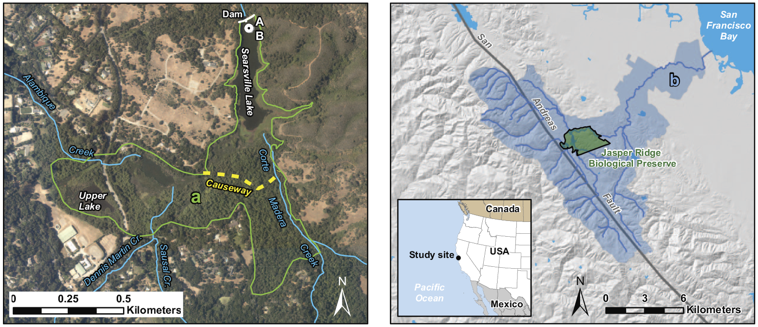
Map of Searsville Lake and the San Francisquito Creek Watershed. Green outline (a) = extent of Searsville in 1892 CE; A = coring location for JRBP2018-VC01A; B = coring location for JRBP2018-VC01B. Blue shaded polygon (b) = San Francisquito watershed; green shaded polygon = Jasper Ridge Biological Preserve; blue lines = creeks. (Map prepared by Trevor Hébert, JRBP). Reproduced in color in online version.

It is ironic that human engineering, the hallmark of the Anthropocene, turned the Searsville site from a riparian valley into a lake whose sediments have archived in great detail the many ways that humans have changed the Earth System. No less ironic is the potential the site holds as the GSSP or “golden spike” for the Anthropocene. In 1869, the founder of Stanford University, Leland Stanford, pounded in the eponymous golden spike to commemorate the completion of the first transcontinental railroad in the USA (Chesley, 2019), a key milestone in the increasing industrialization and globalization that eventually transformed the Holocene world into the Anthropocene world.

Geographic and geologic setting

Searsville Lake and Dam are located at the pinch-point of the San Francisquito Creek watershed, which encompasses approximately 123 km² (Figure 1). The sediments that have filled the majority of the reservoir basin (Freyberg, 2001) are derived from a melange of primarily sedimentary and accreted rocks that range in age from Quaternary to Cretaceous. Movement along the San Andreas Fault has created a steep gradient from the crest of the Santa Cruz Mountains, channelized streams along the NW- to SE-trending fault complex, and has led to fracturing many of the rocks, increasing their friability and contributing to frequent landslides (Kittleson et al., 1996).

The Mediterranean climate of the region features intense downpours in the wet season (generally October to April), followed by a long dry season (Figure 2a), exacerbating expansion and contraction of already-friable rock exposures. During torrential rains in the wet season, the ~20 creeks and their tributaries which comprise the watershed flush vast amounts of material into Searsville Lake, producing a thick sedimentary record in the reservoir that can be resolved to seasons. Over the past 130 years, Searsville Lake has accumulated ~16 m of sediment (~12 cm/year on average), sometimes with several centimeters accumulating in days or even hours during storms (Kittleson et al., 1996). For comparison, sedimentation rates for lakes in the Northeastern United States are typically less than ~0.2 cm/year (Goring et al., 2012).

Figure 2.

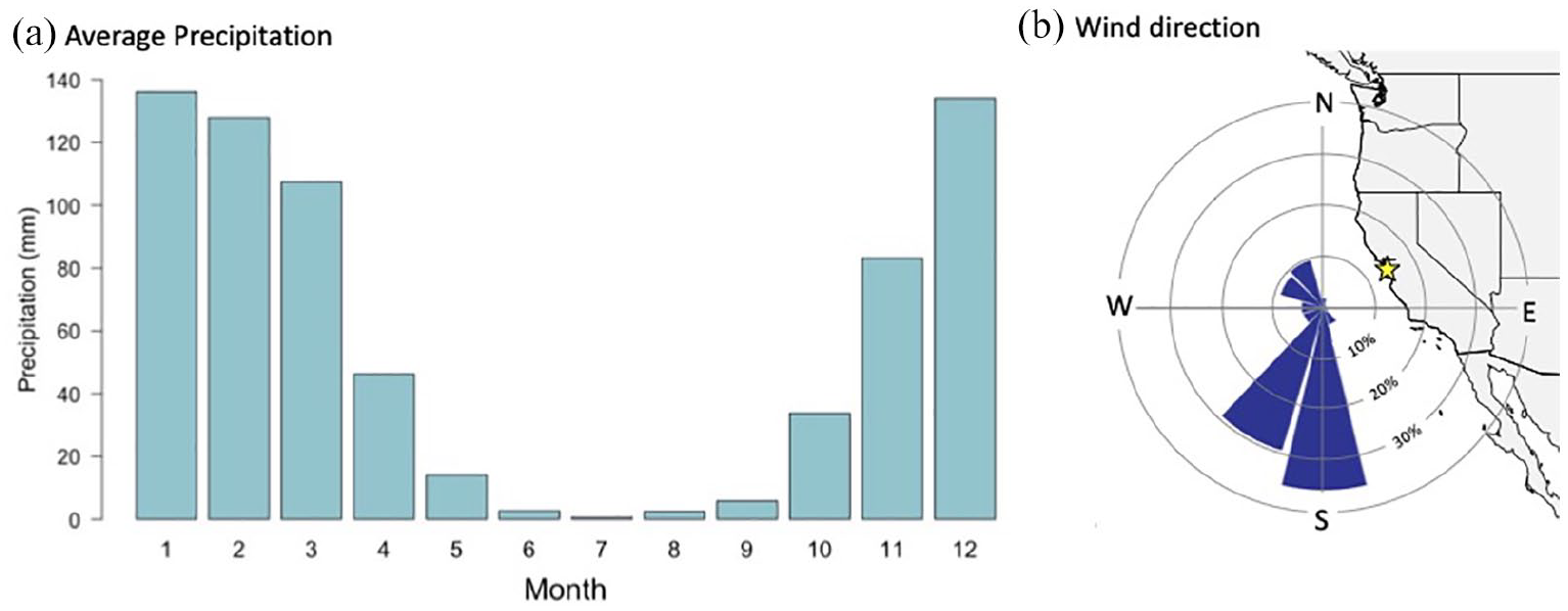
Precipitation and wind direction in the Searsville area. (a) Average monthly precipitation for Woodside, CA and JRBP (1973-2015, from NOAA Station USC00049792 Woodside Fire Station 1; 2015-2022 from JRBP, latitude 37.407128 N, longitude 122.241492 W and latitude 37.405428 N, longitude 122.241492 W) (Data from JRBP, 2022a, 2022b; Menne et al., 2012a, 2012b). (b) Wind direction at Searsville Dam (August 2018 – May 2022, latitude 37.407128 N, longitude 122.241492 W) (Data from JRBP, 2022b). Yellow star indicates the location of JRBP. Reproduced in color in online version.

Pertinent global signals are recorded because just 16 km to the west is the Pacific Ocean (Figure 2b). Global and regional signals are parsed from one another by comparing the geochemical and paleontological changes extracted from the sediments with well-documented archeological records and historical archives (Figure 3; Supplemental 1) (Bocek and Reese, 1992).

Figure 3.

Timeline of social/cultural and land use change in the Searsville region from the mid-1600s to present. Thick/thin lines indicate larger/smaller influence on the landscape. Shaded region shows the time period prior to the construction of Searsville Dam and not captured by Searsville sediments. JRBP = Jasper Ridge Biological Preserve; Red dashed vertical line indicates the proposed GSSP at 1948 CE. (Based on Bocek and Reese, 1992). Reproduced in color in online version.

Accessibility

Searsville Lake is a central feature of Jasper Ridge Biological Preserve, a 485-hectare area within Stanford University that is protected for research, education, and conservation. This ensures that the site will be conserved and protected, but also will remain accessible (Supplemental 1). The sediments in the lake will remain available for additional coring over the next few years, with appropriate permissions from Stanford University and relevant regulatory agencies. In the longer term, Searsville Dam is slated to be modified (Searsville Project Team, 2022) such that the reservoir will be drained and likely expose outcrops of the sediment layers now well-sampled in the cores discussed below (Supplemental 2). The expected new exposures, which would be easily accessible by existing roads and trails, will likely facilitate direct observation of the sediments.

Previous work

The potential value of Searsville sediments as highly resolved sedimentary archives first became evident with nine cores taken by the U.S. Geological Survey in 1998. The information from these cores was never published but was summarized in a white paper provided to JRBP (Berhe et al., 2007; Fries, 1998) where the data and a suite of core photographs are on file. Other research on Searsville Lake extends back nearly a century (Supplemental 1).

Also valuable are archives at JRBP that document information relevant to interpreting sedimentation patterns and anthropogenic inputs into Searsville Lake (Supplemental 1). When the reservoir first formed, it was a continuous body of water that encompassed Middle Lake and Upper Lake, but it rapidly began to fill with sediment. The height of the dam’s spillway varied through time, impacting sediment flux, and in 1929, a levee (the Causeway) was constructed to trap silt in Middle Lake (Figure 1). Nevertheless, infilling of the reservoir continued with a prograding delta from the south. Today, what used to be the southern portion of the original Searsville Lake harbors a riparian forest rich with bird life, and the reservoir itself is less than half its original size, with <10% of its original water storage capacity (Freyberg, 2001).

Materials and methods

Geographical setting of core sites

Ten cores were collected from Searsville Lake in 2018, 2020, and 2022 (Supplemental 2). Two are reported here: JRBP2018-VC01A (latitude 37.406832, longitude −122.237844, datum WGS84; water depth = 265 cm), and JRBP2018-VC01B (latitude 37.406844, longitude −122.237881, datum WGS84; water depth = 268 cm) (Figure 1). Both were collected during the same expedition from the deepest part of the reservoir, approximately 65 m south-southeast of Searsville Dam, and are precisely correlated with each other using physical-stratigraphic and geochemical criteria.

Field collection of core, sampling, and core imagery

JRBP2018-VC01A cores were collected 29–30 October 2018 using a Vibracorer supported by a floating platform. Each core was collected in continuous multiple ~590-cm long aluminum core tubes. JRBP2018-VC01A is 851 cm long with 25.4% compaction ([drive depth–core length]/drive depth) while JRBP2018-VC01B is 944.5 cm long with 14.4% compaction. Depths were originally recorded relative to the drive depth but here are reported relative to the core top, with core top = 0 cm, 252.5 cm below the dam spillway crest which serves as a fixed vertical datum (Supplemental 3). JRBP2018-VC01B was designated as the primary GSSP core and sampled for geochemical markers. JRBP2018-VC01A was used for microfossil sampling and analyses. Both cores were sectioned in the field and JRBP2018-VC01A was also split lengthwise and photographed in the field prior to transport. Cores are stored at the core lab at the USGS Pacific Coastal and Marine Science Center (PCMSC) in Santa Cruz, California, USA. The cores will be permanently reposited at the USGS Southwest Region cold storage facility at Moffett Field in Mountain View, California (USA), where they will be available to future researchers with permission from the USGS (Supplemental 1).

Of the cores taken between 2018 and 2022, five have been split and three of those have been sampled for analyses reported in this paper and/or for other analyses. The remaining five will serve as archives (Supplemental 2). Core scanning was performed in the core lab at the USGS Pacific Coastal and Marine Science Center using a GeoTek Rotating X-ray Computed Tomography (RXCT) and GeoTek Multi-Sensor Core Logger (MSCL). Core sections were CT-scanned at 104-micron resolution using a Thermo Kevex PSX10-65 W X-ray source set to 115 kV and 452 µA. CT scans were reconstructed using Geotek Reconstruction Software. CT intensity is a proxy for sediment density (Holland and Schultheiss, 2014; Tanaka et al., 2011) and is positively correlated with gamma bulk density in JRBP2018-VC01B (Supplemental 4). Linescan core images were collected using a GeoTek Core Imaging system, with a Geoscan V camera. Linescans were collected at 200-micron resolution. JRBP2018-VC01B was scanned for Gamma attenuation using a gamma ray source and detector mounted on the MSCL. JRBP2018-VC01B was CT and gamma attenuation scanned before being split, then immediately line-scanned after splitting. JRBP2018-VC01A was CT scanned as a split core then line-scanned.

X-ray Fluorescence (XRF) data was collected on the MSCL using an Olympus Delta Professional XRF Spectrometer at 1-cm intervals for 20-second measurements per beam, in both Geochem and Soil mode.

Initial visual core descriptions were completed using the Troels-Smith (1955) system for describing organic-rich sediments and the Schnurrenberger et al. (2003) system for classifying lacustrine sediments, including the use of Munsell charts for determining sediment colors.

Grain size distributions were determined from 38 subsamples (31 from JRBP2018-VC01B, 7 from JRBP2018-VC01A) at the US Geological Survey Pacific Coastal and Marine Science Center (Supplemental 5). Samples were selected to represent the range of sediment density observed in both cores.

CT, line scan, XRF, gamma density, and grain size data are published in an accompanying USGS Data Release (La Selle et al., 2023).

Chronological controls

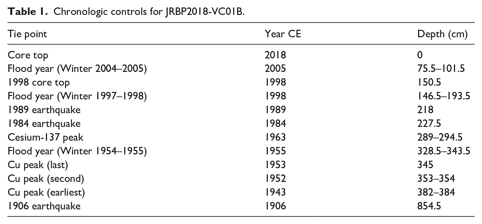
The highly resolved chronology for JRBP2018-VC01B was constructed using a combination of seasonal-layer counting enabled by distinctive wet-season/dry-season couplets, distinctive sedimentary features, radiometric tie-points (Cesium-137), and correlation of historic event and climate data to geochemical (copper (Cu), calcium (Ca), and titanium (Ti)) and sedimentological signals (1906 and 1989 earthquakes) in the cores (Supplemental 1).

We identified chronological anchor points that could be tied with precision to particular years, including: the top of the core (October 2018), sedimentary features indicative of the 1989 Loma Prieta and 1906 San Francisco earthquakes (evident as disturbed layers in otherwise regularly layered sediments), the 1963 ¹³⁷Cs spike (Supplemental 6), and documented historical inputs to the lake which were detected in the XRF scans (Table 1). Those inputs were the use of the algaecide copper sulfate (CuSO₄) from 1943 to 1947 at a rate of 300 lbs per week beginning in the spring each year (Erwin, 1947; Jones, 2021), and again in 1952 and 1953 when 10 t of copper sulfate were applied (JRBP Archives, 1953). Chloride of lime, or calcium hypochlorite (Ca(ClO)₂), was also used to control algae from as early as the 1930s (Felin, 1940) and through the 1940s (Erwin, 1947; Jones, 2021) and corresponds to Ca peaks in the XRF data from ~431.5 to 761.5 cm.

Table 1.

Chronologic controls for JRBP2018-VC01B.

Tie point	Year CE	Depth (cm)
Core top	2018	0
Flood year (Winter 2004–2005)	2005	75.5–101.5
1998 core top	1998	150.5
Flood year (Winter 1997–1998)	1998	146.5–193.5
1989 earthquake	1989	218
1984 earthquake	1984	227.5
Cesium-137 peak	1963	289–294.5
Flood year (Winter 1954–1955)	1955	328.5–343.5
Cu peak (last)	1953	345
Cu peak (second)	1952	353–354
Cu peak (earliest)	1943	382–384
1906 earthquake	1906	854.5

We used the XRF Ti profile and CT scans to count annual wet- and dry-season layers (Figure 4; Supplemental 1 and 7). Previous studies have demonstrated a strong relationship between XRF-measured Ti in sediment cores and rainfall/runoff (Haug et al., 2001; Hendy et al., 2015; Peterson and Haug, 2006), and Ti is correlated with precipitation and stream runoff in Searsville as well (Supplemental 1). Ti has been used to confirm or count varves in other studies (Hendy et al., 2015; Kienel et al., 2009).

Figure 4.

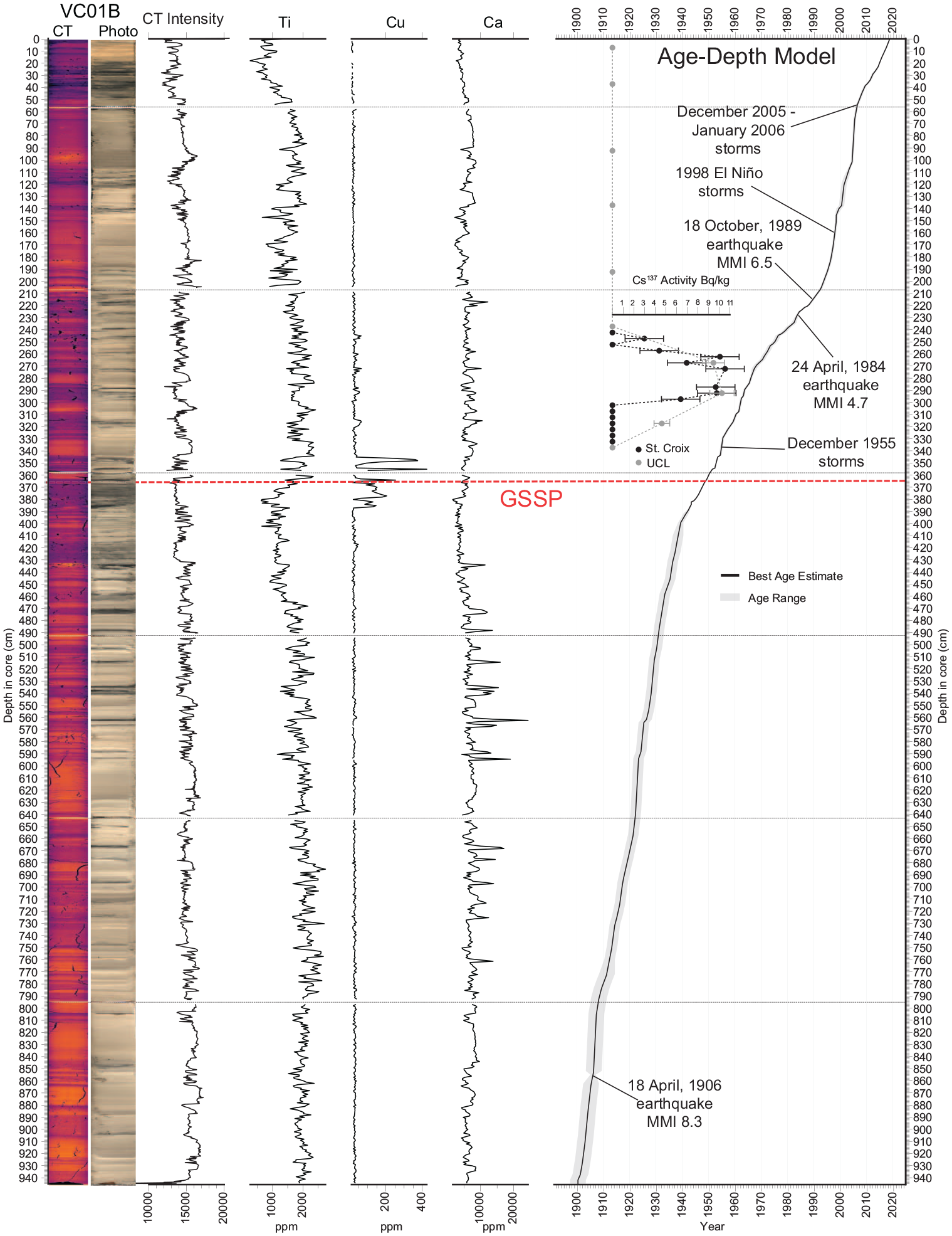
Searsville core JRBP2018-VC01B CT, XRF, ¹³⁷Cs, and age model. From left to right: CT scan; photo; average CT intensity; XRF Ti, Cu, and Ca; ¹³⁷Cs; and age-depth model. Red dashed horizontal line indicates the proposed GSSP depth at 366 cm (1948 CE). Reproduced in color in online version.

The age model for JRBP2018-VC01A was constructed by detailed matching of the layers evident in CT scans to those also evident in JRBP2018-VC01B, and by alignment of Cu and Ca peaks in the XRF scans from the two cores (Supplemental 8). The variation in thickness of layers of varying CT intensity from top to bottom of each core results in a clear pattern, analogous to paleomagnetic stripe-patterns.

Anthropocene radioisotopes

Freeze-dried sediment samples from JRBP2018-VC01B were analyzed for Americium-241 while measuring Lead-210 and ¹³⁷Cs by direct gamma assay in the Environmental Radiometric Facility at University College London (see Methods: Chronological Controls; Supplemental 6).

We analyzed 19 bulk sediment samples for bomb radiocarbon by Accelerator Mass Spectrometry at the Laboratory of Ion Beam Physics, ETH Zürich. Samples were collected from JRBP2018-VC01B at depths between 359.5 to 0 cm. Radiocarbon ages were calibrated using the IntCal20 calibration curve (Reimer et al., 2020) in the Bchron (Haslett and Parnell, 2008) package in R (R Core Team, 2021).

Plutonium-239,240 activities and isotope ratios were analyzed in freeze-dried sediment samples from between 379.5 to 4 cm in JRBP2018-VC01B. Some adjacent samples were combined to increase sample sizes and one sample was subsequently excluded from our study because it was from a storm deposit which would have been deposited over only a few days. This sample was from the same depth as one excluded from our ¹³⁷Cs dataset. ^239,240Pu activities were analyzed (following total sample dissolution by borate fusion and radiochemical separation) via alpha spectrometry at the GAU-Radioanalytical Laboratories at the University of Southampton. Samples analyzed for ^239,240Pu activities were later re-dissolved and analyzed via MC-ICPMS to determine ²⁴⁰Pu/²³⁹Pu ratios (Supplemental 9).

Novel materials

Spheroidal carbonaceous particles

Sixty-eight samples from JRBP2018-VC01B between 934.5 and 9.5 cm were collected and freeze dried for spheroidal carbonaceous particle (SCP) analysis at University College London. The sampling interval ranged from 5 to 30 cm, with the highest density of samples between 379.5 and 189 cm. Sediment samples were analyzed for SCPs following the method described in Rose (1994) and the criteria for SCP identification under the light microscope followed Rose (2008). During counting, SCPs were subdivided into size classes (4–10, 10–25, 25–50, and 50–75 µm). Sediment blanks and SCP reference material (Rose, 2008) were included in each digestion. Detection limits for this analysis were typically 250–300 g DM⁻¹ (per gram dry mass of sediment) (Supplemental 10).

Polychlorinated biphenyls

Sediment samples for polychlorinated biphenyl (PCB) analysis were collected at 16-cm increments, then aggregated into 6 combined, depth-averaged samples to achieve adequate sample size (Supplemental 11). Samples were analyzed at PHYSIS Environmental Laboratories, Inc. (Anaheim, California, USA) following method EPA 8270D (EPA, 1998) to detect PCB congeners and concentrations.

Organic matter proxies

Carbon (C) and nitrogen (N) bulk elemental and isotopic analyses were performed at the Stanford Stable Isotope Biogeochemistry Laboratory (SIBL) (Stanford, California, USA) on samples from between 944 and 3.5 cm of JRBP2018-VC01B (Supplemental 12).

To model trends in organic matter proxies we used Generalized Additive Models (GAMs) with adaptive splines and restricted maximum likelihood (REML), following the guidance of Simpson (2018) and implemented in the mgcv package (Wood, 2011, 2017) in R (R Core Team, 2021). We identified significant increases/decreases in our GAMs by locating regions where the derivative of the GAM was significantly different from zero, using the “derivatives” function in the R gratia package (Simpson, 2022). We tested for correlation between organic matter proxies and depth using Spearman’s correlation, and also tested for changes in variance of organic matter proxies in rolling windows of 10 samples, using Spearman’s rank correlations.

Inorganic geochemical signals

Major and trace element content of JRBP2018-VC01B was analyzed by inductively coupled plasma mass spectrometry (ICPMS; Supplemental 13). Twenty of the samples analyzed for major and trace element content were also analyzed for lead isotopes (²⁰⁴Pb, ²⁰⁶Pb, ²⁰⁷Pb, and ²⁰⁸Pb). Pb was isolated from bulk rock dissolutions using HBr-based chemistry on AG1x8 anion exchange resin. Samples were analyzed on the Agilent 8900 ICPMS and were corrected for instrumental mass fractionation using sample-standard bracketing with NIST SRM-981. External reproducibility is based on repeated analysis of the USGS BHVO2 basalt standard over the three analytical sessions (n = 8).

For mercury (Hg), samples of ~0.3 g and 0.5 cm thick were collected at 5 cm intervals starting at a base depth of 944.5 cm, and analyzed in triplicate at the Stanford Carnegie Institute Department of Global Ecology by thermal decomposition followed by preconcentration of Hg on a gold trap and cold vapor atomic absorption spectrophotometry using a DMA-80 direct Hg analyzer (Milestone, CT, USA) (Supplemental 14). See Redondo (2022) for further details.

We modeled trends in inorganic geochemical signals using the same GAM modeling method described for organic matter proxies.

Biotic markers

Samples for biotic marker analysis were collected from Searsville core JRBP2018-VC01A at overlapping depths and in the low-density sediment layers associated with higher organic matter.

Ostracods and cladocera ephippia

For ostracod and cladoceran analysis, 28 sediment samples of ~15 g and 2 cm thickness were collected from JRBP2018-VC01A. Samples were washed through a set of nested sieves (300, 180, and 100 μm) and air dried, then picked under a dissecting microscope and mounted on micropaleontology slides following the methods of Horne and Siveter (2016). The specimens were sorted into morphotypes under a compound microscope. Ostracod valves less than ~50% complete were logged but not included in analyses (see Supplemental 15 and Viteri (2022) for further details).

Diatoms

For diatom analysis, 40 sediment samples of ~5 cm³ volume and spanning between 2 and 8 cm depth were collected from JRBP2018-VC01A. Diatom samples were processed at the National Lacustrine Core Facility (LacCore; University of Minnesota, Minneapolis, Minnesota, USA). Processing constituted digestion of the organic matter and carbonates in the sediment using peroxide and hydrochloric acid (HCl) (Supplemental 15).

Pollen, spores, and non-pollen palynomorphs

Pollen analysis was conducted on 40 samples from JRBP2018-VC10A at the same depths as for diatoms at the Northern Arizona University Laboratory of Paleoecology (NAU LOP; Flagstaff, Arizona, USA) (Supplemental 16).

Pollen and spores mounted on microscope slides were identified at 400× magnification to a ~300 terrestrial grain sum (exclusive of wetland and aquatic types, spores and non-pollen palynomorphs (NPPs); tracer counts varied from 248 to 7,419). Identifications were made to the lowest taxonomic level possible, usually genus, sometimes family, generic groupings or family groupings, based on published keys (e.g. Fægri and Iversen, 1989; McAndrews et al., 1973; Moore et al., 1991; Reille, 1992), and the NAU LOP pollen reference collection (Supplemental 16). The NPPs were identified based on van Hoeve and Hendrikse (1998), van Geel et al. (2001), Ejarque et al. (2015), Anderson et al. (2015), and the website http://non-pollen-palynomorphs.uni-goettingen.de. Some aquatic NPPs (algae, rotifers, and protozoa) were used in an additional analysis with cladocerans and ostracods.

Results

Lithology

The Searsville cores are fairly homogeneous gray to brown silt and clay (Figure 5) interspersed with some dark black bands which were visible immediately after core splitting but have since faded. The CT scans show discrete layers ranging from <1 mm to >30 cm thick, with no evidence of bioturbation or hiatuses.

Figure 5.

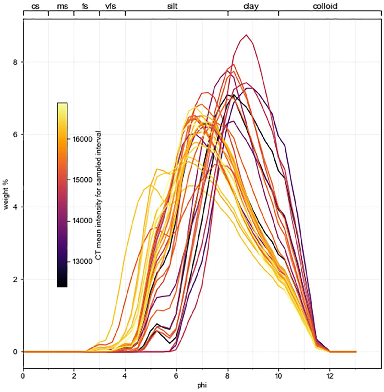
Searsville core JRBP2018-VC01B grain size. Color indicates CT intensity at the depths associated with each grain size sample. Each line represents the weight % grain size of a single sample. Reproduced in color in online version.

The grain size distributions of sediments from wet seasons are typically moderately sorted with D50 medians (the median particle size) in silt. The inorganic components of dry season sediments consist of well sorted clay-sized particles. Higher deposition rates during wet seasons resulted in massive or thickly laminated silts with normal grading occurring in the upper 0.1–3.0 cm of the beds. The relationship between median grain size and 1-cm mean CT intensities is linear. Layers with a median grain size in coarser silt have CT intensities greater than 15,000, while clay-dominated layers have CT intensities less than 15,000.

Chronology

Depositional rates are highly variable from season to season in Searsville Lake. This is a huge advantage for developing a detailed chronology as described above but complicates the application of dating techniques that rely on uniform depositional rates, notably ²¹⁰Pb dating, which was uninformative (Supplemental 1).

¹³⁷Cs was first detected at 319.5–314 cm (4.64 ± 0.78 Bq/kg). It then increased upcore to 294.5–289 cm and remained elevated until 246.5–259.5 cm before declining sharply. The youngest ¹³⁷Cs detection was at 249.5–244.5 cm (2.99 ± 1.85 Bq/kg). Above this point ¹³⁷Cs activity concentration dropped below detection limit of the gamma-spectrometric measurement. Our two rounds of analyses identified two potential peaks: the first analysis indicated peak ¹³⁷Cs at 294.5–289 cm (10.28 ± 1.19 Bq/kq) while the second analysis suggested the peak at 274.5–269.5 cm (10.57 ± 1.85 Bq/kg). The error bars of the two peaks overlap. We used several lines of evidence to determine which peak likely corresponds to the year 1963 CE. First, counting of annual layers supports the lower depth, 294.5–289 cm, as 1963 CE. Layer counts in this part of the core are well-constrained by the XRF Cu peaks from 1943-1953 CE and by the 1955 CE flood deposit. Second, although it is possible for ¹³⁷Cs to be mobilized from anoxic sediments, it would move up into younger deposits, not down into older sediments (Comans et al., 1989). We therefore conclude that the sediments at 294.5–289 cm of the core formed in 1963 CE when there was a maximum ¹³⁷Cs fallout derived from nuclear weapons testing (Appleby, 2001).

Seasonal layer counting, verified by Ti profiles and visual inspection of CT scans, indicates 118 ± 3 annual layers in JRBP2018-VC01B. This information, combined with the chronological anchors described in the Methods section above and Supplemental 1, places the base of core at 1900 ± 3 CE and the top at 2018 CE (Figure 4). Age error ranged between ±0.25 and ±3 years. For layers where the year could be determined with a high level of confidence based on sedimentological or geochemical evidence of historically recorded events (e.g. 1906, 1943, 1963, 1989, 2018 CE), we assigned an error of ±0.25 year to account for the fact that the onset of the wet and dry seasons can vary by several months depending on the year (Table 1). In general, where seasonal layers were clear and independent tie points were denser, error bars were ±1 year. However, in segments of the core that represented winters with little or no rain, seasonal layering was less clear, resulting in error bars that were generally considered to be from ±1 to 2 years. Below the Cu peak in 1943, error bars increased to ±2–3 years (Supplemental 1). The 1906 earthquake layer also served to constrain the bottom age of the core, as did correlation with the 1998 cores that included pre-reservoir soil.

Seasonal layer counting and matching of Ca patterns in the XRF demonstrated that the base of JRBP2018-VC01A was deposited during the same year and season as the base of JRBP2018-VC01B.

Calculation of sedimentation rates

Because of the episodic sedimentation events, sedimentation rates were highly variable, ranging from 1 to 47.5 cm/year with a mean of 15.6 cm/year and median of 12 cm/year (Supplemental 17). Rates were generally higher before ~391 cm (pre-1940s CE, mean = 19.5 cm/year). Rates slowed from ~391 to ~191 cm (~1940 to 1995 CE; mean = 5.3 cm/year), increased again from ~191 to 51 cm (~1995 to 2007 CE; mean = 18.0 cm/year), then once again slowed from 51 cm to the top of the core (2007–2018 CE, mean = 4.8 cm/year).

Radioisotopes

²⁴¹Am Only one ²⁴¹Am activity value of 1.24 ± 0.64 Bq/kg was detected at 9.5–4 cm (2016 ± 0.25–2018 ± 0.25 CE). The source of this is not well understood; however, because there is an in-growth of ²⁴¹Am from ²⁴¹Pu decay, recent catchment in-wash could be elevated in ²⁴¹Am. Maximum ²⁴¹Am in-growth takes about 70 years (Malátová and Bečková, 2014), so peak ²⁴¹Am levels could be observed within the next 10 years or so in Searsville.

¹⁴C

Radiocarbon ages for JRBP2018-VC01B bulk sediments were all much older than the known age of the reservoir, and age did not increase with depth, probably because sediments contained old carbon from coal-bearing sedimentary rocks upstream (Supplemental 1 and 18).

²³⁹Pu and ²⁴⁰Pu

Samples were analyzed from depths ranging from 379.5 to 4 cm in JRBP2018-VC01B. Low levels of ^239,240Pu were found in all samples except the combined sample from 379.5 to 374 cm (1945 ± 0.25 to 1946 ± 0.25 CE). The first ^239,240Pu detection was in a sample that spanned depths 374–372 cm (1946 ± 0.25–1947 ± 0.25; 0.0120 ± 0.0080 Bq/kg) (Figure 6). We found three notable peaks in ^239,240Pu across the record: the first at 319.5–314 cm (1958 ± 0.5–1959 ± 0.5 CE; 0.3842 ± 0.0886 Bq/kg), the second and highest at 294.5–289 cm (1963 CE; 0.7526 ± 0.1481 Bq/kg), and the last at 244.5–244 cm (1976 ± 0.5–1977 ± 1 CE; 0.3911 ± 0.0708 Bq/kg). The first two peaks correspond closely in age to peaks in ^239,240Pu fallout documented in Hancock et al. (2014). A sample from 254.5 to 249 cm was contaminated and excluded from our analysis. Samples from 316.5 to 266.5 cm (1959 ± 0.5 to 1969 ± 1 CE), the depth interval with maximum ^239,240Pu activities, had ²⁴⁰Pu/²³⁹Pu ratios between 0.18 and 0.22 (Supplemental 9). These are consistent with ratios previously reported for global nuclear weapons fallout in northern latitudes (Wu et al., 2011). Samples from other depth increments had very low CPS (counts per second) of 3000 or less, below reliable determination levels.

Figure 6.

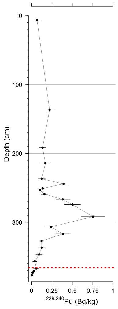
Searsville core JRBP2018-VC01B ^239,240Pu activities. Red dashed horizontal line indicates the proposed GSSP depth at 366 cm (1948 CE). Error bars are shown as solid horizontal lines. Reproduced in color in online version.

Novel materials

SCPs

The first SCPs were found at 449.5–449 cm (1934 ± 2 CE) (Figure 7). Above this, SCP concentrations were irregular, and absent in 14 out of 51 samples. Throughout the core SCP concentrations were low with peak concentrations exceeding 1600 gDM⁻¹ at 264.5–264 (1970 ± 1 CE) and 2000 gDM⁻¹ at 254.5–254 cm (1973 ± 1 CE). Low SCP concentrations are likely due to the high sedimentation rates in this reservoir.

Figure 7.

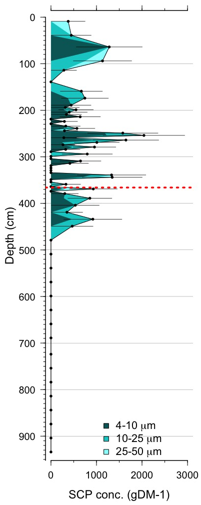
Searsville core JRBP2018-VC01B spheroidal carbonaceous particle concentrations. Red dashed horizontal line indicates the proposed GSSP depth at 366 cm (1948 CE). Reproduced in color in online version.

The SCP profile shows some similar features to other North American cores, for example, an increase in SCPs in sediments in the 1930s, peaking in the 1970s and lower concentrations persisting through to today (Rose, 2015). Most SCPs fell in the 4–10 µm size range, but some SCPs in slightly larger fractions occurred throughout (Figure 7, Supplemental 10). No SCPs >50 µm were observed, suggesting that a nearby source of SCPs is less likely (Inoue et al., 2013). Searsville Lake is not downwind of any local coal-burning power stations, suggesting that the deposition of the SCPs is a regional, not local, signature.

PCBs

PCBs were not detected in samples below 461.5 cm (pre-1930s) (Supplemental 11). Above this depth, one congener (PCB 153) was found in the sediment from 461.5 to 316.5 cm (1933 ± 2 to 1959 ± 0.5 CE), seven congeners (PCB 149, 153, 174, 180, 183, and 187) were found from 301.5 to 156.5 cm (1962 ± 0.5 to 1998 ± 0.5 CE), and two congeners (PCB 149 and 153) were found from 141.5 to 0.5 cm (1998 ± 1 to 2018 ± 0.25 CE). Total PCB concentrations (0.612, 2.571, and 0.33 ng/g in the first, second, and third samples from the top, respectively) were relatively low as compared to other lake sediment cores (Bigus et al., 2014). PCBs were commercially produced between 1930 and 1980 (Bigus et al., 2014), so the pattern of PCB increase and decline in our core matches this history closely.

Organic matter proxies

Total organic carbon (TOC)

TOC ranged from 1.29 to 3.34% and increased with some plateaus after ~520 cm (~1929 ± CE) to the top of the core (Spearman’s rho = −0.67, p-value < 1 × 10⁻¹⁵), with peaks at depths of 434–419 (1936 ± 2–1937 ± 2 CE), 104 (2004 ± 0.5 CE), and 39 cm (2008 ± 0.5 CE) (Figure 8; Supplemental 12). Variance also significantly increased from the bottom to the top of the core (Spearman’s rho = −0.83, p-value < 1 × 10⁻¹⁵)

Figure 8.

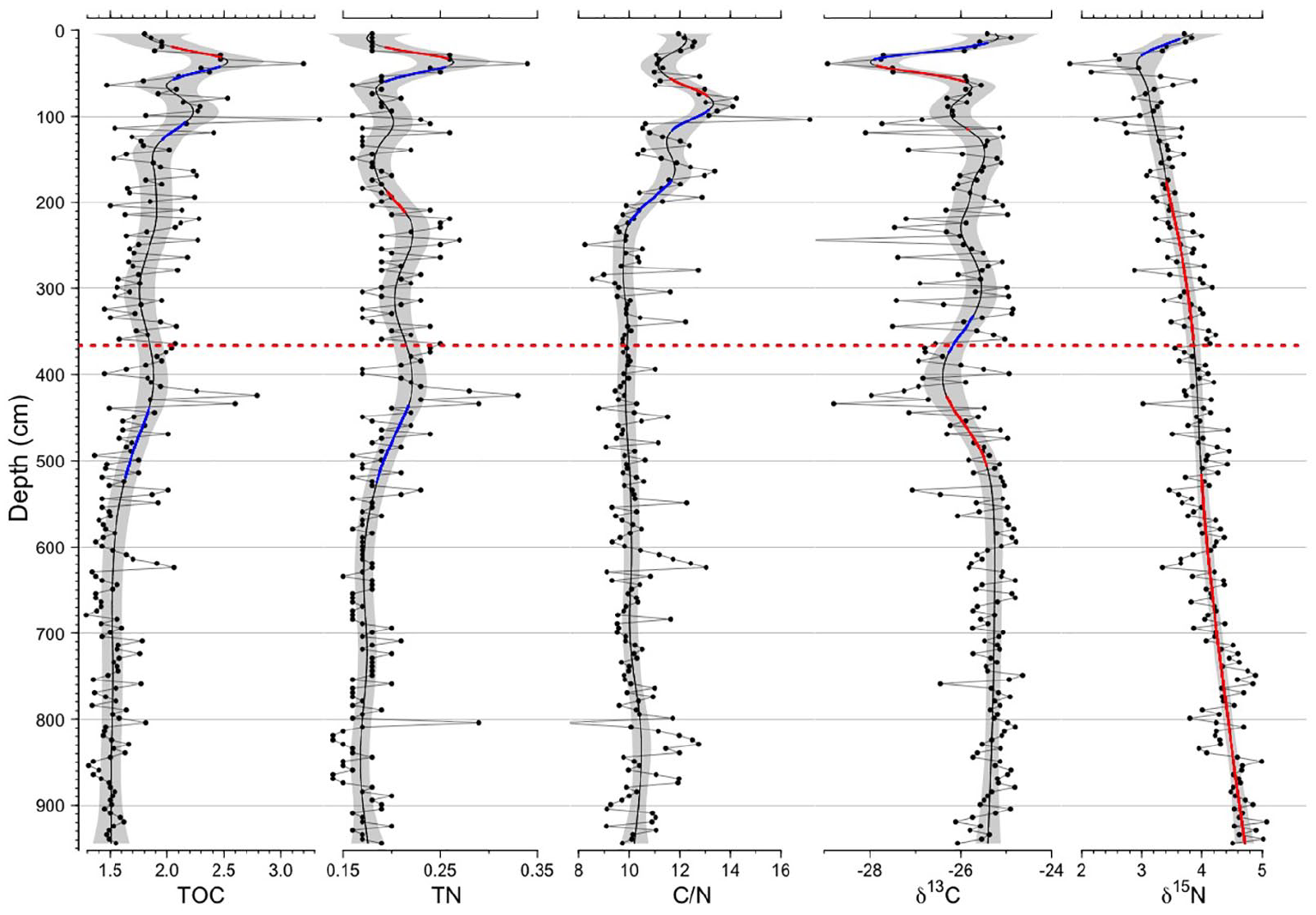
Searsville core JRBP2018-VC01B organic matter proxies. From left to right: total organic carbon (TOC), total nitrogen (TN), carbon/nitrogen ratio (C/N), δ¹³C, and δ¹⁵N. Gray shading show the GAM model 95% confidence interval. Solid blue/red lines show GAM significant increases/decreases. Red dashed horizontal line indicates the proposed GSSP depth at 366 cm (1948 CE). Reproduced in color in online version.

Total nitrogen (TN)

TN ranged from 0.14 to 0.34% and generally increased from the bottom to the top of the core (Spearman’s rho = −0.49, p-value < 1 × 10⁻¹²) but notable increase started around 520 cm (~1929 ±2 CE) (Figure 8; Supplemental 12). After that, TN fluctuated through time and was relatively elevated from ~441.5 to 366.5 (1935 ± 2 – 1948 ± 0.25 CE), 261.5–211.5 (1971 ± 1–1990 ± 0.5 CE), 121.5–101.5 (2001 ± 1–2004 ± 0.5 CE), and 51.5–21.5 cm (2007 ± 0.5–2014 ± 0.25 CE). Variance also significantly increased from the bottom to the top of the core (Spearman’s rho = −0.48, p-value < 1 × 10⁻¹⁰), but particularly above ~491.5 cm (1931 ± 2 CE).

C/N ratio

C/N mass ratio values ranged from 7.23 to 17.15 (Figure 8; Supplemental 12) and although it was weakly correlated with depth (Spearman’s rho = −0.29, p-value < 1×10⁻⁴), significant increases in C/N did not begin until ~210 cm (~1991 ± 0.5 CE). Below 210 cm, mean C/N ratio was 10.20 but above the mean increased to 11.98.

Stable carbon isotopes (δ¹³C)

δ¹³C ranged from −24.64 to −29.42 and was fairly stable from the bottom of the core up to ~510 cm (~1929 ±2 CE), with a mean of −26.11 (95% confidence interval = −26.36 − 24.81) (Figure 8; Supplemental 12). Above 510 cm, δ¹³C values became more variable and more depleted on average (mean = − 26.11 above 510, vs −25.35 below 510 cm). This is also reflected in the significant correlation between depth and variance (Spearman’s rho = −0.72, p-value < 1 × 10⁻¹⁵). The decline in δ¹³C beginning at ~1929 CE is about 36 years earlier than the typical inflection point for δ¹³C evident globally, suggesting local influences at Searsville override the global pattern. The most notable decline in δ¹³C was found near the top of the core, from ~51.5 to 21.5 cm (~2007 ±0.5–2014 ± 0.25 CE), but this was followed by a sharp increase to the top of the core.

Stable nitrogen isotopes (δ¹⁵N)

δ¹⁵N ranged from 1.81 to 5.08 and generally declined from the bottom to the top of the core, except for a brief increase above ~30 cm (2012 ± 0.5 CE) (Spearman’s rho = 0.84, p-value < 1 × 10⁻¹⁵) (Figure 8; Supplemental 12). Variance also increased through time, but this was driven by values above ~140 cm (~1999 ±1 CE): if values above 140 cm are removed, there is no significant relationship between depth and δ¹⁵N variance. This decline generally mirrors the pattern in lake sediments elsewhere (Wolfe et al., 2013).

Inorganic geochemical signals

Given the high sedimentation rates in Searsville, the majority of heavy metals are likely entering the lake through geological material eroded from the watershed. However, fluctuations in heavy metals through time could be caused by either changes in the source rocks being eroded, changes in atmospheric deposition, or both. Changes in the source of erosional material are expected to cause coordinated changes in the concentration of elements, including heavy metals, in the sediment—that is, a simultaneous increase/decrease reflecting a shift in mineral composition. Because in many cases we do not see coordinated changes in heavy metal composition, it is likely that changes in anthropogenic deposition via the atmosphere is an additional source. Here we note trends in Pb, Hg, and several other heavy metals which may document anthropogenic pollution. Full ICPMS results can be found in Supplemental 13.

Pb

Lead concentration ranged from 11 to 32 ppm over the core (Figure 9). Values were low and fairly stable from the bottom of the core to ~540 cm (1928 ± 2 CE), varying between 11 and 19 ppm. From ~540 to ~415 cm (1928 ± 2 to 1938 ± 2 CE), Pb concentration increased significantly to the first of two major peaks (maximum = 26 ppm) at ~430–400 cm (1936 ± 2–1938 ± 1 CE). The GAM model suggests no significant increase or decrease from 400 to ~210, but two peaks in Pb were seen in this span, one at 264–263.5 cm (30 ppm; 1970 ± 1 CE) and the second at 224–223.5 cm (32 ppm; 1985 ± 0.5 CE). Pb then declined significantly from ~210 to ~120 cm (1991 ± 0.5 – 2001 ± 1 CE), returning to early 1900s values and remaining low to the top of the core (range = 11–18 ppm).

Figure 9.

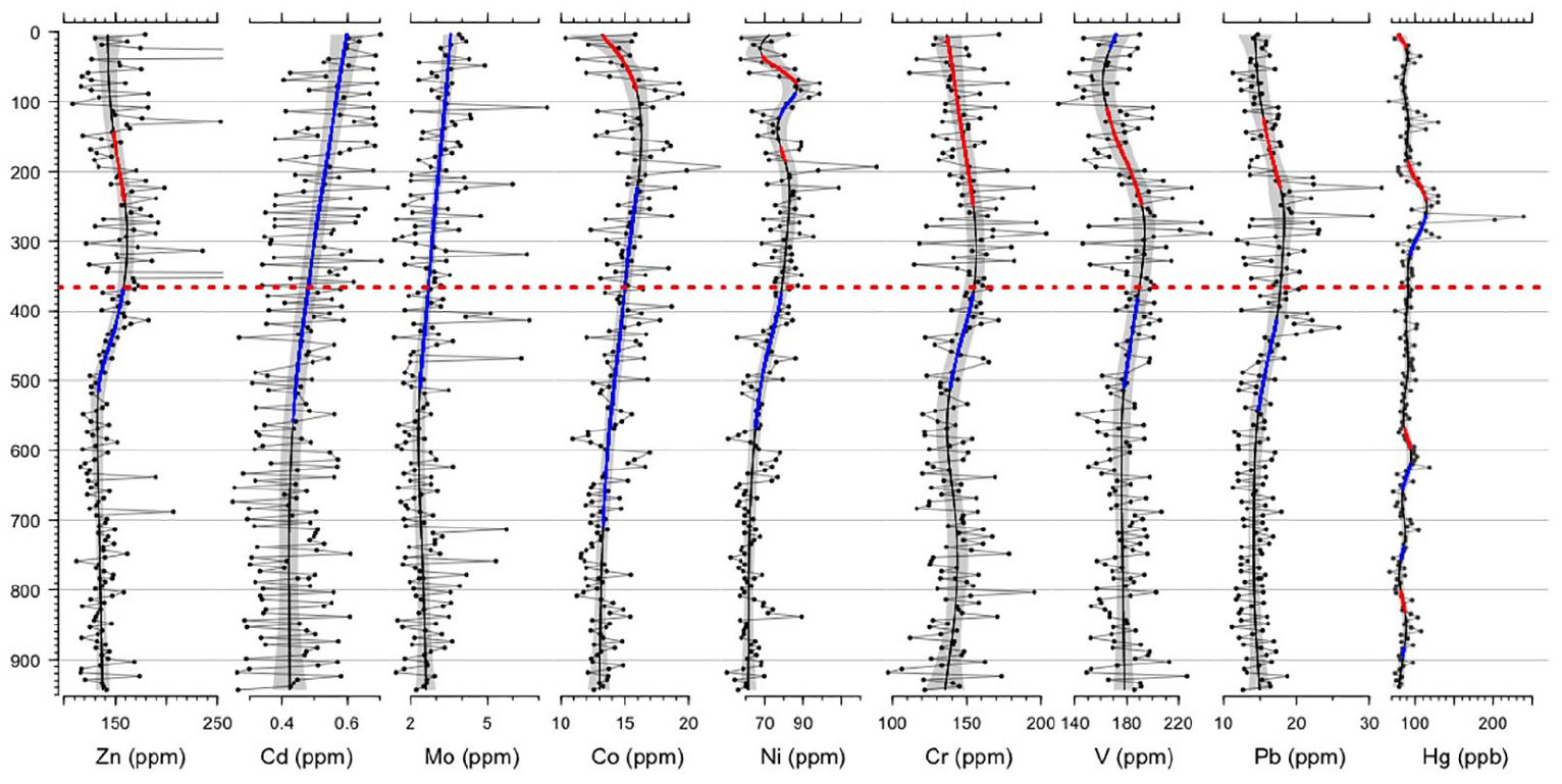
Searsville core JRBP2018-VC01B heavy metals. From left to right: zinc (Zn), cadmium (Cd), molybdenum (Mo), cobalt (Co), nickel (Ni), chromium (Cr), vanadium (V), lead (Pb), and mercury (Hg). Gray shading shows the GAM model 95% confidence interval. Solid blue/red lines shows GAM significant increases/decreases. Red dashed horizontal line indicates the proposed GSSP depth at 366 cm (1948 CE). Two extreme Zn values (348.5 cm, 639 ppm; 33.5 cm, 744 ppm) were removed for scale. Reproduced in color in online version.

All sediment samples tested had Pb isotopes with strongly overlapping error bars (Supplemental 13). These samples fell in the range of natural background (Ritson et al., 1999).

Hg

The average Hg concentration for Searsville sediments was 91.7 ppb (ng/g) (Figure 9). This represents significant elevation over pre-1860 baseline values of ~47 ppb on average, as evidenced by Hg values from an Upper Lake Marsh core (Redondo, 2022). Hg concentration fluctuated throughout the core. Notable peaks and valleys, where values were more than one standard deviation above/below the mean were evident (Figure 9). At 624.5 cm (1922 ± 2 CE), Hg concentration was 118.7 ppb. The highest levels were seen in adjacent samples at 269.5 (201.9 ppb; 1967 ± 2 CE) and 264.5 cm (239.3 ppb, 1970 ± 1 CE). Elevated concentrations were also seen before and after this major peak, from ~294 to ~224 cm (~1963 ± 0.5 to 1985 ± 0.5 CE). Following this, Hg concentration decreased toward the present, with one rebound at 129.5 cm (129.3 ppb; 2000 ± 1 CE). The lowest concentrations recorded for the Searsville core were found at 99.5 cm (66.6 ppb; 2004 ± 0.5 CE) and 774.5 cm (67.6 ppb; 1910 ± 3 CE).

Other heavy metals

Heavy metal concentrations in the Searsville core follow a sequence of increases throughout the 20th century (Figure 9). Cadmium (Cd) increased continuously from ~560 cm (~1926± 2 CE) to the top of the core, later than expected based on annual global production estimates (Han et al., 2002) and concentrations in Greenland ice cores (Candelone et al., 1995; McConnell and Edwards, 2008), but on par with Cd measured in Siberian and Chilean alpine ice cores (Eichler et al., 2014; Potocki et al., 2022). Molybdenum (Mo) increased from ~510 cm (~1929± 2 CE) to the top of the core, also closely matching the rise in global Mo production (Henckens et al., 2018) and measurements of Mo from alpine ice cores (Arienzo et al., 2021). Cobalt (Co), nickel (Ni), chromium (Cr), vanadium (V), and zinc (Zn) followed a different pattern, first increasing significantly–beginning at ~708 cm (1916 ± 2 CE) for Co, ~720 cm (1926 ± 2 CE) for Ni, ~510 cm (1929 ± 2 CE) for Cr and V, and ~ 515 cm (1929 ± 2 CE) for Zn–then declining again–beginning at ~240 cm (~2005 CE) for Co, ~230 cm (2005 ± 0.5 CE) for Ni, ~248 cm (1975 ± 1 CE) for Cr and V, and ~240 cm (1979 ± 1 CE) for Zn. Ni shows a brief decrease and then increase from ~184 to 89 cm (1996 ± 0.5to 2004 ± 0.5 CE). The vast majority of Co is produced as a byproduct of other metals including Ni and Cu (Slack et al., 2017) so increases in Co might be expected to track trends in other metals. However, in Searsville, the increase in Co is later than the onset of major global Cu or Ni production (Han et al., 2002). Increases in Cr and Ni in Searsville closely match the onset of major global production, but the subsequent decline in both elements differs from the global record (Han et al., 2002). In a study of an alpine ice core, Van de Velde et al. (1999) found that Co, Cr, and Mo all increased in the 1940s, however no samples were analyzed between the 1920s and 1940s. Nevertheless, this suggests that our observed increase in Co in Searsville may reflect global atmospheric increases. Co production declined in the mid-1980s, matching the timing of our decline in Searsville, though we do not recover the expected increase in the 2000s (Slack et al., 2017). Vanadium (V) in Searsville tracks the rise and then fall of V detected in alpine ice cores in Western Europe, linked to petroleum consumption (Arienzo et al., 2021), and V emissions reported since 1950 (Bai et al., 2021). Zn increase in Searsville is later than increases in global emissions, but the decline matches emissions reductions post-1980 (Nriagu, 1996).

Biotic markers

Ostracods, cladocera, and diatoms

In total, 407 ostracod valves and 466 ephippia were recovered from core JRBP2018-VC01A (Viteri, 2022). Unidentifiable early juvenile ostracod molts (instars) comprise 74.0% of ostracod valves in our study (Figure 10). Among the identifiable valves, the major constituents of the ostracod assemblage were Physocypria globula (53.8%) and Candona spp (30.8%). The remaining constituents, Ilyocypris cf. gibba (6.7%), Cypria cf. ophthalmica (3.8%), Cypridopsis vidua (2.9%), and Pseudocandona spp. (1.9) are relatively rare. Cypria cf. ophthalmica occurred only in youngest levels above 75 cm (2002 ± 1 CE) while Ilyocypris cf. gibba was only in levels older than 1950 CE. All taxa are considered cosmopolitan (Smith and Delorme, 2010).

Figure 10.

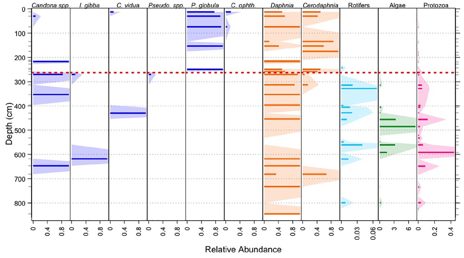
Searsville core JRBP2018-VC01A microcrustaceans and plankton. Relative abundance of Ostracods (blue; Pseudo. spp. = Pseudocandona spp., C. vidua = Cypridopsis vidua, C. ophth. = Cypria ophthalmica, I. gibba = Ilyocypris cf. gibba, P. globula = Physocypria globula) and Cladoceran ephippia (orange); and rotifers (turquoise), algae (green), and protozoa (pink) abundance relative to the terrestrial pollen sum. Red dashed horizontal line indicates the proposed GSSP year, 1948 CE. Silhouette is 3× exaggeration. Reproduced in color in online version.

Ephippia from the cladoceran Daphnia spp. occur throughout the core. Those from Ceriodaphnia spp. make a brief appearance low in the core, at 682–680 cm (1909 ± 3 CE), are absent until 314–312 cm (1937 ± 2 years), then increase markedly in abundance at 259–257 cm depth (1950 ± 0.5–1951 ± 0.5 CE), above which high abundance is sustained.

Diatoms were rare, highly dissolved, or absent in all JRBP2018-VC01A processed samples (Supplemental 1 and 15).

Pollen, spores, and non-pollen palynomorphs

Sequoia sempervirens (coast redwood), Quercus (oak) sp. and Pseudotsuga menziesii (Douglas-fir) each increased over the course of the record, with some fluctuations (Figure 11). Other tree types occurring less consistently include Lithocarpus (tanoak), Pinus cf. radiata (Monterey pine), Umbellularia californica (California Bay), Aesculus californica (California buckeye), Juglans (walnut), Acer (maple), and Betula (pendula [European white birch] / occidentalis [water]). The introduced tree species Eucalyptus (blue gum) and Olea (olive) are found through the record, while Ulmus (americana [eastern]/parviflora [Chinese] elm) and Ailanthus altissima (tree-of-heaven) first appeared at 708–705 (~1907 ± 3 CE) and 274– 269 cm (~1943 ± 0.5–1947 ± 0.25 CE) respectively.

Figure 11.

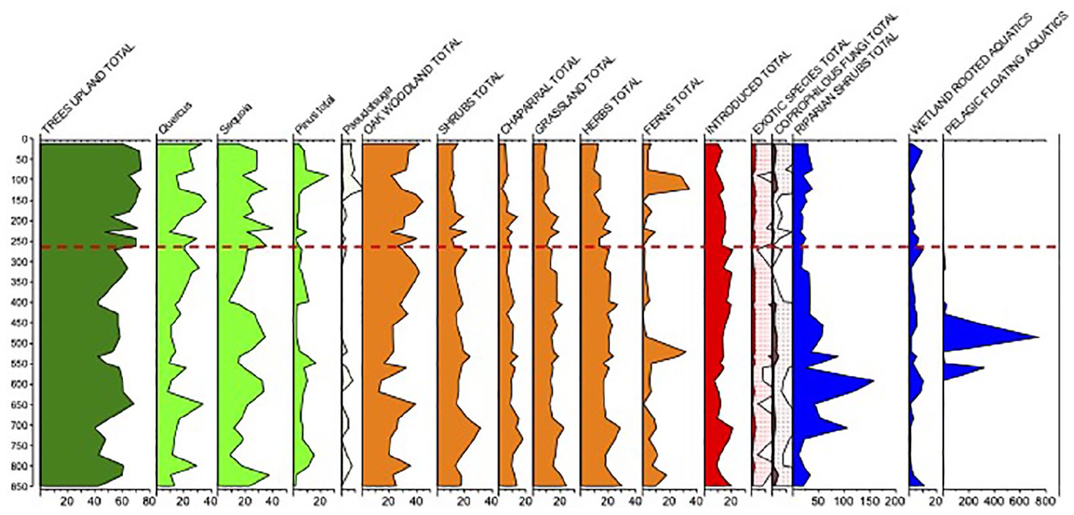
Pollen percentages of dominant taxa and major functional groups from the Searsville core JRBP2018-VC01A. The Trees Upland Total includes pollen of Sequoia, Taxaceae-Cupressaceae group, Pseudotsuga, Pinus total (where identified, P. cf radiata), Quercus, Lithocarpus, Umbellularia, Olea/Ligustrum, Eucalyptus, Juglans, Betula, Aesculus, Ailanthus, Acer, Ulmus, Fraxinus, Populus, Platanus, Carya and Tilia. Red dashed horizontal line indicates the proposed GSSP year at 1948 CE. Reproduced in color in online version.

Shrub pollen types include those that decrease through time, such as Asteraceae and Rhus (lemonade bush); those that remain mostly consistent through time, such as Artemisia (sagebrush), the Ericaceae (probably Arctostaphylos) and Rhamnus (buckthorn); those that increase, such as Ceanothus (California lilac) and Chrysolepis (chinquapin); and others that occur more sporadically (Corylus cf. cornuta (hazel), and Rosaceae (rose) family, and others). Common herbs are the Poaceae (grass family), with introduced ruderals such as the Amaranthaceae (goosefoot family), Plantago (plantain), and Rumex (dock), all of which were present at the beginning of the record. Poaceae increased from 594 to 425 cm (1917 ± 2 to 1928 ± 2 CE), then declined after 216 cm (1960 ± 0.5 CE). Ruderals were also less abundant above ~241 cm (~1953 CE). Introduced cereal grains (Cerealia, including species Secale [rye] and Zea [maize]) occurred regularly below ~271 cm (~1946 CE), but were less common above. Additional pollen types from introduced species include: Apiaceae, Erodium, and Fabaceae (first occurrence: 846–851 cm; 1900 ± 3 CE); Lactuceae (825–821 cm; 1902 ± 3 CE); Brassicaceae (801–797 cm; 1903 ± 3 CE); Galium (738–731 cm; 1906 ± 3 CE); Acacia (688–680 cm; 1908 ± 3–1909 ± 3 CE); Lathyrus (651–646 cm; 1912 ± 2 CE); and Portulaca (523–520 cm; 1922 ± 2 CE). Ferns were found throughout but were most abundant below 520 cm (1922 ± 2 CE) and from 126 to 88 cm (1993 ± 0.5 to 2000 ± 1 CE).

Among the wetland species, Alnus rhombifolia (white alder) generally increased from the bottom of the core to 589 cm (1917 ± 2 CE), then declined and persisted. Salix (willow) peaked in abundance from 521.5 to 328 cm (1922 ± 2 to 1936 ± 2 CE), then declined sharply. Cyperaceae (sedge family), Typha latifolia (cattail), and the aquatic macrophytes Sparganium (bur-reed) and Isoetes (quillwort) were all present throughout the record while Equisetum (horsetail) and Azolla (water fern) were found only sporadically, and Potamogeton (pondweed) and Brasenia shreberi (watershield) were rare. Myriophyllum (watermilfoil), possibly either a native or introduced species, was found only from 619 to 398 cm (1915 ± 2 to 1930 ± 2 CE) while native Polygonum amphibium (water knotweed) was found from 243 to 137 cm (1953 ± 0.5 to 1985 ± 0.5 CE).

Algae were most common below ~260 cm (~1950 CE). Notably, Debarya had a large peak at 594–589 cm (1917 ± 2 CE) and Pediastrum peaked three times between 563 and 453 cm (1919 ± 2 to 1925 ± 2 CE), but both were uncommon subsequently. In general, algae and rotifers crashed in abundance at ~260 cm (~1950 CE) and subsequently did not recover. Protozoa show a marked decline at the same level (Figure 10).

Discussion

Satisfying criteria for defining a GSSP

The Searsville site satisfies all the criteria ideal for defining a GSSP (Supplemental 1). The core we propose for the GSSP (JRBP2018-VC01B) is 944.5 cm long, encompassing 118 years from 1900 to 2018 CE. The ~50 years prior to our proposed boundary are represented by 578.5 cm of sediment, while the ~50 years following the boundary span 366 cm. This very thick and continuous sequence means that our GSSP boundary, and the appearance and fluctuations in the primary and auxiliary markers, can be mapped to particular years (and even in some cases within a season) with a high level of confidence.

Primary marker

We propose the primary marker for the Anthropocene GSSP to be the first widespread appearance of ^239,240Pu. In JRBP2018-VC01B, the first evidence of ^239,240Pu occurs at 374–372 cm, which corresponds to late 1946 and early 1947 CE. This is consistent with the earliest history of nuclear detonations and the 1–2 years lag-time between ejection of plutonium into the atmosphere and incorporation globally into geologic deposits (Supplemental 1). Note that we did not use the ^239,240Pu profile to help develop our age model. Because of the demonstrated lag time between nuclear explosions and global deposition of radionuclides, appearance of Pu in multiple geological sites around the world after 1948 CE is more likely than appearance in multiple sites by 1945 (three detonations), 1946 (two detonations), or 1947 (no detonations), making a date after 1948 a more practical choice for the Anthropocene GSSP and its chronostratigraphic beginning. Therefore, using ^239,240Pu as the primary marker and guide, we propose the base of the Anthropocene be set at a depth of 366 cm in Searsville Lake core JRBP2018-VC01B, corresponding to October-December of 1948. In Searsville cores this depth is easily recognizable as the top of a very dark gray/black layer approximately 1 cm-thick, and it is also distinct in CT scans as a sharp <1 mm-thick boundary between low- and high-density sediment (Figure 12). Local rainfall records show that the first rainfall in the summer/fall of 1948 occurred on October 3 and precipitation continued sporadically through the end of the year, so the wet season sediments above the boundary at 366 cm were deposited sometime between October and December 1948, capping dry season sediments which accumulated in the summer of 1948.

Figure 12.

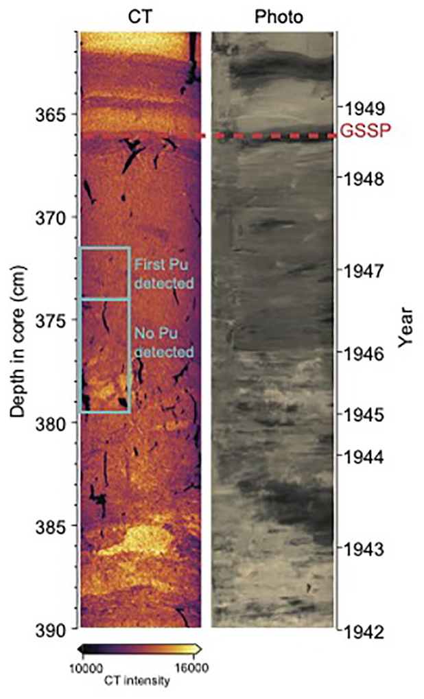
Detail of Searsville Core JRBP2018-VC01B GSSP boundary. CT scan (left); photo (right); red dashed line = GSSP depth, 366 cm (1948 CE). Reproduced in color in online version.

At Searsville, the sediments track the rise in atmospheric ^239,240Pu concentrations in the 1950s, with an early peak in 1958/1959 CE, followed by a decline, matching the timing of the 1959 nuclear weapons testing moratorium (Waters et al., 2015). This temporary low point in Searsville ^239,240Pu concentrations corresponds to 1961 CE, the year that testing resumed (Waters et al., 2015). Following peak testing in 1962 CE (Waters et al., 2015), ^239,240Pu peaks in the Searsville sediments at 1963 CE. This supports the conclusion that Searsville sediments, like those from other deposits around the world, document atmospheric fallout from testing with a lag of 1 to 2 years, on par with the 1.5 ± 0.5 year residence time of Pu in the atmosphere (Hirose and Povinec, 2015). The ²⁴⁰Pu/²³⁹Pu isotope ratio confirms that the signal in Searsville Lake is from global nuclear atmospheric testing fallout (Wu et al., 2011).

Global auxiliary markers

The Searsville cores JRBP2018-VC01B and -VC01A (taken only a few meters apart and and tightly correlated to one another) demonstrate several auxiliary markers that can be used to recognize Anthropocene deposits worldwide (Figure 13).

Figure 13.

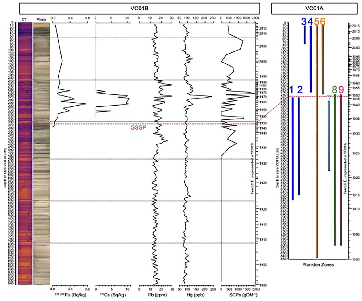
Selected Searsville Lake global (^239,240Pu, ¹³⁷Cs), global/regional (Pb, Hg, SCPs), and local (microcrustacean and plankton zones) signals. Red dashed horizontal line indicates the proposed GSSP year at 1948 CE. High abundance (>10%) zones for Candona spp. (1), rotifers (7), algae (8), and protozoa (9); High abundance and persistence zones for Physocypria globula (4) and Ceriodaphnia (6); and occurrence zones for Ilyocypris gibba (2), Cypria ophthalmica (3), and Daphnia (5). (Colors match Figure 10). Reproduced in color in online version.

Radionuclides

¹³⁷Cs

The Searsville record exhibits a clear ¹³⁷Cs signal, with earliest detection at levels corresponding to 1958 CE and a peak recognized at 1963 CE. Therefore, we specify the presence of ¹³⁷Cs as a reliable auxiliary marker for the Anthropocene.

Novel material proxies

Spheroidal carbonaceous particles (SCPs)

The first presence of SCPs in the Searsville core are recorded in the mid-1930s. Concentrations were variable afterward and low overall, most likely reflecting more distant rather than local sources and dilution due to high sediment accumulation rates (Supplemental 10). The SCP size profile was typical (<50 µm) for sites not located in the immediate vicinity of a source (Rose, 2008). In view of this, we regard SCPs in Searsville as reflecting a regional rather than local signal. Searsville also conforms to other records that indicate the first appearance of SCPs prior to the mid-20th century. At Searsville, SCPs first appear ~14 years prior to our suggested start date of the Anthropocene. However, SCPs clearly document a critical signal of anthropogenic impacts. This signal may become most useful as an auxiliary marker by using the rapid increase in SCP accumulation (Rose, 2015) rather than first appearance which varies considerable around the world.

Polychlorinated biphenyls (PCBs)

A single PCB congener makes its appearance in the Searsville record between 1933 and 1959 CE, consistent with the timing of their first commercial production in 1929 and subsequent increase (Markowitz, 2018). Multiple congeners occur in the record in levels dating from 1959 to 2018, with peak abundance in the depth-averaged sample dating to between 1962 and 1998, reflecting the pattern of increasing use, then decline following the ban of PCB manufacturing in the United States in 1979 (Markowitz, 2018) and internationally in 2001 (Porta and Zumeta, 2002). Similar patterns can be expected in other lake deposits; thus, we recognize the presence of multiple congeners of PCBs as an auxiliary marker. PCB sources generally will be local rather than global, but their use was so pervasive in the late 20th century that many lake and soil deposits can be expected to contain detectable quantities.

Organic matter proxies

Stable nitrogen isotopes (δ¹⁵N)

Declines in δ¹⁵N are caused by burning of fossil fuels and synthetic fertilizer production, which increase reactive nitrogen. The effect of fossil fuel burning on δ¹⁵N started in the 1800s, before the accumulation of sediments in Searsville, while production of synthetic fertilizer started in earnest in the 1920s (Waters et al., 2016). We observed the expected steady decline in δ¹⁵N in Searville through time, with a decline in average values of ~1.8 per mil. Precipitation is considered a major source of δ¹⁵N (Talbot, 2001). Because storm systems on the West Coast of North America come over the Pacific, the δ¹⁵N in Searsville almost certainly reflects the atmospheric signal. Because global reactive N increased gradually over the last ~200 years (Waters et al., 2016), profiles typically do not show a pronounced inflection point near mid-century. However, we suggest that δ¹⁵N profiles may prove useful as auxiliary Anthropocene markers by recognizing the point at which the δ¹⁵N values decline by at least half over the time period 1900–2000 CE. For the Searsville profile, this point is reached at ~1950 CE. This use of an auxiliary marker will be most useful when: (1) diagenesis is not an issue, as is the case in Searsville, and (2) when the time scale in question spans the 20th century.

Inorganic geochemical signals

Lead (Pb)

The Pb profiles for Searsville closely mirror the increasing input of Pb into the atmosphere, especially from increasing use of leaded gasoline and other fossil fuels that began in ~1930, peaked in the 1970s, and then declined as unleaded gasoline became the norm. At Searsville, the highest peaks in Pb occur in levels corresponding to 1970–1985, indicating that peaks in Pb profiles will provide a useful auxiliary marker to help identify Anthropocene sediments deposited from the late 1960s to the 1980s.

Mercury (Hg)

Hg concentration in Searsville was roughly double the pre-industrial Hg concentration in Upper Lake Marsh (Redondo, 2022), suggesting a major increase in Hg deposition over the last century that is consistent with global and North American patterns of Hg production and consumption (Horowitz et al., 2014; Streets et al., 2019; Zhang et al., 2016). The largest Hg signal in the Searsville core occurred from ~1967 to 1970, coincident with peak Hg mine production (Han et al., 2002) and U.S. Hg consumption patterns (Horowitz et al., 2014). Elevated Hg can therefore be used to identify sediments deposited during the post-industrial time, and peak Hg, corresponding to the late 1960s and early 1970s, can identify deposits as securely in the Anthropocene.

Other heavy metals

Changes in heavy metals in Searsville could reflect changes in erosional sources and/or changes in atmospheric deposition. V is the most abundant metal in petroleum (Amorim et al., 2007) and increases in V have been shown to track petroleum consumption (Arienzo et al., 2021). The increase in V in Searsville began around 1930, consistent with the rise in petroleum production and consumption (Hughes and Rudolph, 2011). The Searsville record also tracks industrial production of Cr, Ni, and Mo, which began to increase in the mid-1920s/early 1930s (Han et al., 2002; Henckens et al., 2018). Increased concentrations of these heavy metals are apparent in Searsville sediments dating younger than 1948 CE (Figure 9).

Paleoclimate proxies

The seasonally deposited layering in the Searsville sediments provides a first-order climatic proxy, which can be matched in detail with tree-ring records from nearby blue oaks (Quercus douglassi) and other high-resolution climate proxies (Supplemental 1). Given patterns of anthropogenic climate change that begin to become apparent in the mid- to late-20th century, it is likely that such detailed climatic proxies will prove useful as auxiliary Anthropocene markers, even though proxies and signals may differ from site to site. Although climate change has been and will continue to be expressed differently regionally, the consequences of climate change are part of a global suite of changes which are recognizably associated with the Anthropocene.

Regional and local auxiliary markers

Stable carbon isotopes (δ¹³C)

Carbon isotope records from ice cores, which reflect the global atmospheric signature (Rubino et al., 2013, 2019), typically show declining δ¹³C through the 20th century with an inflection point and steeper decline in the 1960s. At Searsville, we instead see a decline in mean δ¹³C starting in the 1930s, possibly caused in part by atmospheric depletion from fossil fuel burning, that is coupled with an increase in the variability. The Searsville record likely differs from ice core records because ice samples the air directly, whereas lake sediments also record the δ¹³C of organic material deposited in the lake (Supplemental 12). For this reason, we do not regard carbon isotopes as providing an effective auxiliary marker at Searsville, though δ¹³C likely will be useful in other kinds of deposits.

Paleobiologic proxies

Paleontological evidence that typically characterizes epoch/series boundaries include First and Last Appearance Datums (FADs and LADs, respectively), range zones (typically defined by the FAD and LAD of a particular taxon), concurrent-range zones (overlapping ranges of multiple species), interval zones (defined on FAD and LAD of different taxa), lineage zones (defined by a specific segment of an evolutionary lineage), and abundance zones (based on varying abundances of taxa).

As is the case for most sedimentary records younger than ~10,000 years, at Searsville auxiliary markers that rely on FADs of newly evolved species are not evident, given that most species on Earth today originated long before the 20th century. However, FADs of immigrant taxa can be useful regionally (Himson et al., 2021; Williams et al., 2022). At Searsville, Cypria cf. ophthalmica, which makes its first appearance near the top of the record at 75–73 cm (corresponding to 2002–2003 CE) in JRBP2018-VC01A, may provide a useful FAD for recognizing Anthropocene parts of the section. The pollen record documents many non-native plant species, but all were introduced to the area prior to the accumulation of Searsville sediments. Ongoing work to extract sedimentary DNA (sedaDNA) shows promise for establishing a chronology of introduced invasive species (Supplemental 1).

LADs caused by extinction are not evident in the Searsville record or others of similar age for reasons noted in Supplemental 1. However, Holocene and Anthropocene sediments may be distinguished on the basis of local and regional species disappearances. At Searsville, a useful local LAD is the loss of the ostracod Ilyocypris cf. gibba, which drops out of the JRBP2018-VC01A record around 1948 CE. This corresponds to our proposed Holocene-Anthropocene boundary based on earliest evidence of Pu, as defined above, making the absence of I. gibba a useful auxiliary marker locally.

Local abundance zones hold promise as auxiliary markers for identifying the position of the Holocene-Anthropocene boundary within Searsville. Candona spp. is the most abundant ostracod taxon in sediments deposited below 269 cm (1947 CE), while Physocypria globula is the most abundant ostracod taxon subsequently, first appearing at 250–248 cm (~1952 CE) and becoming abundant above ~154 cm (~1976 CE). Thus, the replacement of Candona spp. by P. globula marks the Anthropocene-Holocene boundary at Searsville (Supplemental 1). Below ~436 cm, ostracod counts are too low to draw meaningful relative abundance conclusions. Also above the proposed Holocene-Anthropocene boundary, cladoceran taxa occur at approximately equal relative percentages, whereas below, Daphnia usually dominates over Ceriodaphnia. Both taxa decline in absolute abundance in the Anthropocene (Supplemental 1). The proposed Holocene-Anthropocene boundary also clearly coincides with the locally rapid decline of rotifers, algae, and protozoa (Figure 10). Accordingly, we recognize a P. globula abundance zone from 248 cm (fall/winter 1952± 0.75 CE) to the top of the core (characterized by high P. globula abundance) as identifying Anthropocene sediments at Searsville. A local rotifer-algae-protozoa abundance zone from the bottom of the core to 269 cm (summer of 1947 CE; characterized by relatively abundant rotifers, algae, and protozoa) identifies Holocene sediments, and pronounced decline or lack of those taxa above 264 cm (mid-1948 CE) identifies Anthropocene sediments. Relatively equal percentages of Daphnia and Ceriodaphnia also appear useful in characterizing the post-1948 sediments. While the specific taxa involved in these zones may only apply locally at Searsville, we expect that other deposits exhibit contemporaneous changes in microfossil assemblages as a result of intensifying anthropogenic activities in their watersheds.

The terrestrial pollen record in Searsville also illustrates increasing human resource use at a local scale, mirroring shifts that took place regionally and globally. For example, the abundance changes document the rebound of coast redwood (Sequoia sempervirens) and Douglas-fir (Pseudotsuga menziesii) after cessation of logging and grazing, respectively (Supplemental 1; Anderson et al., in review). The usefulness of such changes in the upland vegetation as auxiliary markers for the Anthropocene is limited at Searsville, as they do not coincide with a Holocene-Anthropocene boundary set at the mid-20th century. However, in general, the influence of anthropogenic land-use on vegetation is clear, which is a common finding in most pollen records of the 20th century. Changes to riparian, wetland, and aquatic vegetation, on the other hand, were abrupt and staggered from the ~1920s into the ~1940s (Figure 11), in part influenced by construction activities that emplaced a levee or altered the height of the dam (Supplemental 1; Anderson et al., in review).

In sum, the paleobiologic proxies at Searsville are useful in locally differentiating proposed Anthropocene layers from underlying Holocene sediments. While the patterns result from local modifications in the Searsville watershed and therefore may not extend regionally, they reflect a general feature of the Great Acceleration: intensification of anthropogenic inputs, which may well be expected in contemporaneous deposits elsewhere.

Searsvillian Stage and Age

The recognition of the Anthropocene GSSP in the Searsville Lake deposits would warrant definition of the Searsvillian Stage/Age. This stage/age is named with reference to Searsville Lake, in turn named for the historic town of Searsville. The GSSP and primary marker (^239,240Pu) and auxiliary markers for the Searsvillian Stage/Age would correspond to those we propose for the Anthropocene GSSP at Searsville. Like the Anthropocene, the Searsvillian Stage/Age would begin in 1948 CE. This boundary accordingly would mark the end of the preceding Meghalayan Stage/Age.

Conclusions

The Searsville Lake site exhibits all the features ideal for recognizing the GSSP for the Anthropocene. The structurally undisturbed sediments are thick with a rapid sedimentation rate, continuous with no facies changes over the critical interval, dated with high precision (seasonally to annually) throughout the sequence, span the critical interval, and they contain well-studied, clear primary and auxiliary markers.

The best primary marker is the presence of globally deposited ^239,240Pu, which has a robust signature at Searsville and first appears in late 1946 CE, as early as can be expected for a globally relevant ^239,240Pu signal. The Searsville GSSP would place the beginning of the Anthropocene in late 1948 CE, above the first ^239,240Pu and corresponding to clear sedimentological signals.

Auxiliary markers in geochemical and sedimentary profiles include the presence of ¹³⁷Cs; relatively low values of δ¹⁵N; and relatively high values of mercury and lead, spheroidal carbonaceous particles (SCPs) and polychlorinated biphenyls (PCBs), all of which are consistent with documented global signatures and/or with expectations of sedimentary signatures of the Great Acceleration.

Paleontological auxiliary markers include a very strong local signal of an abrupt relative-abundance shift of various ostracod and cladoceran taxa, and in rotifers, algae, and protozoa, all of which coincide with the proposed Holocene-Anthropocene boundary at Searsville. The abundance shifts in Searsville microfauna reflect the local manifestation of increasing anthropogenic influence in watersheds globally that accelerated in the mid-20th century. Therefore, while the exact species involved may differ in other sites, Holocene-to-Anthropocene abundance shifts in local microfauna species might be expected in many lake deposits worldwide that are adequately sampled. Palynological data reflect anthropogenic transformations of the surrounding area, documenting the long history of local anthropogenic impacts, a general feature of pollen records worldwide, and facilitate correlation to other sites in the region that have produced pollen records.

Relevant geochemical signals found in Searsville are also found in other lakes, peat deposits, marine sediments, corals, speleothems, trees, and ice cores (Waters et al., 2023). Paleontological markers (matched through chains of correlation) can apply to marine and freshwater deposits. High-resolution correlation of the annually resolved Searsville sediment record with nearby tree-ring paleoclimate proxies records, already underway, can link the Searsville record to recent climate change. Additional studies underway that will further aid in correlation include using sedimentary DNA to pinpoint the first arrival of neobiota, and geochemical and paleontological data to match the Searsville sediments with their marine counterparts in nearby San Francisco Bay.

In addition to the geological and geochemical attributes of the Searsville site, it is located within Stanford University’s Jasper Ridge Biological Preserve, with a long and successful history of facilitating research, education, and preservation. This ensures continued access to the site by researchers and students, and it will remain a focal point for communication and outreach to the general public. The sediments that have been analyzed so far are duplicated in at least 10 archival cores, and in the short term, more cores can be obtained with appropriate permissions from Stanford and pertinent regulatory agencies. Future plans to decommission the dam will likely result in well-exposed outcrops that would further facilitate access, study, and communication about this most recent transition of the Earth System into the Anthropocene.

Supplemental Material

sj-docx-1-anr-10.1177_20530196221144098 – Supplemental material for The Searsville Lake Site (California, USA) as a candidate Global Boundary Stratotype Section and Point for the Anthropocene Series

Supplemental material, sj-docx-1-anr-10.1177_20530196221144098 for The Searsville Lake Site (California, USA) as a candidate Global Boundary Stratotype Section and Point for the Anthropocene Series by M Allison Stegner, Elizabeth A Hadly, Anthony D Barnosky, SeanPaul La Selle, Brian Sherrod, R Scott Anderson, Sergio A Redondo, Maria C Viteri, Karrie L Weaver, Andrew B Cundy, Pawel Gaca, Neil L Rose, Handong Yang, Sarah L Roberts, Irka Hajdas, Bryan A Black and Trisha L Spanbauer in The Anthropocene Review

Supplemental Material

sj-csv-2-anr-10.1177_20530196221144098 – Supplemental material for The Searsville Lake Site (California, USA) as a candidate Global Boundary Stratotype Section and Point for the Anthropocene Series

Supplemental material, sj-csv-2-anr-10.1177_20530196221144098 for The Searsville Lake Site (California, USA) as a candidate Global Boundary Stratotype Section and Point for the Anthropocene Series by M Allison Stegner, Elizabeth A Hadly, Anthony D Barnosky, SeanPaul La Selle, Brian Sherrod, R Scott Anderson, Sergio A Redondo, Maria C Viteri, Karrie L Weaver, Andrew B Cundy, Pawel Gaca, Neil L Rose, Handong Yang, Sarah L Roberts, Irka Hajdas, Bryan A Black and Trisha L Spanbauer in The Anthropocene Review