
Abstract
Global trade is a neglected topic in debates on the Anthropocene, but plays an implicit role in several suggested definitions of it. Trade’s role in shifting environmental burdens around the globe differed substantially between the Columbian Exchange (1492−1800), the Industrial Revolution (~1800−1950) and the Great Acceleration (post-1950). However, this systematic state-of-the-art review shows that the more than 350 global studies of trade-embedded environmental factors all centre on the Great Acceleration. An underlying concern here is whether environmental factor flows are to the economic and/or environmental benefit of all, a case of the rich exploiting the poor, or merely the inadvertent consequence of differences in environmental efficiency. We point out similarities in the trends and direction of flows between major world regions and between developed and developing countries. Factors such as land, virtual water, HANPP and eutrophying pollutants that are related to the organic economy (or direct biomass flows), primarily flow from regions where population density is low to where it is high, and are only secondarily affected by affluence. Indicators such as energy, airborne pollutant emissions and greenhouse gasses that are related to the mineral economy (fossil fuel, metal and mineral use) tend to flow from developing to developed countries, and are explained either by higher consumption rates or greater environmental efficiency in affluent countries, which has similar consequences for net flows. We weave the shifting trends and directions of flows during the Great Acceleration into a coherent story. Finally, returning to the period before the Great Acceleration, we argue the need for global studies of trade-embedded factor flows before 1950 to test ideas on the character and origins of the Anthropocene, and to accomplish this suggest either geographically extending quantitative long-term national and/or commodity studies, or environmentally extending recently compiled global monetary bilateral trade data for the pre-1950 period.
Keywords
Introduction
The study of global trade-embedded environmental factors tries to unite the study of humanity’s global environmental impact with that of the global integration and division of production and consumption. It adopts an expanding flora of environmental indicators or ‘factors’, including materials or energy contained within traded goods (‘direct flows’), or materials, land, water, energy, pollutants and greenhouse gasses (GHG) used or emitted in their production (‘indirect flows’) (Arto et al., 2012; Malik et al., 2019; Moran et al., 2013; Wiedmann and Lenzen, 2018) and is central in many current debates on carbon leakage, pollution havens, unequal exchange, the environmental Kuznets curve, dematerialisation and food-, resource- and water-security.
Global trade has also been an at least implicit prerequisite in many definitions of the Anthropocene, partly following from the self-imposed constraint that environmental impact must be both synchronous and global in extent. Three periods suggested as the origin of the Anthropocene correspond to different periods of globalisation. First, the Columbian Exchange between 1492 and 1800 signalled the origins of globalisation by connecting Eurasia and Africa with the Americas and Oceania economically, epidemically and ecologically (Crosby, 2003; De Zwart and Van Zanden, 2018; Lewis and Maslin, 2018; Mann, 2011; Polónia and Pacheco, 2017). Trade volumes and trade’s share of GDP were still small (Figure 1), however, and rather than the transfer of resources (cf. Nichols and Gogineni, 2018: 113) global trade’s role in environmental impact consisted primarily in the transfer of (live) species, including crops, diseases and people (notably African slaves and their crops; Carney and Rosomoff, 2017), resulting in biological homogenisation and persistent changes in the global distribution of species (Lewis and Maslin, 2015a, 2015b, 2018; cf. Zalasiewicz et al., 2015).
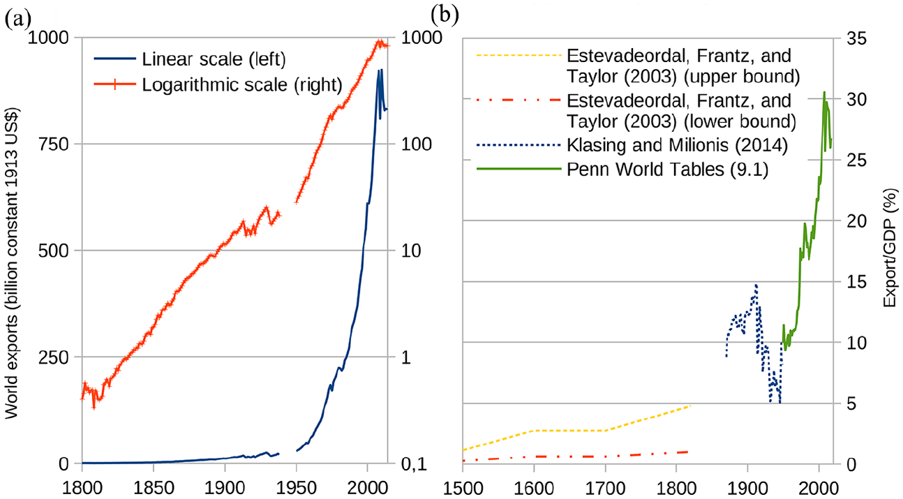
Volume and GDP-share of world trade. (a) Volume of world trade. (b) World export share of GDP.
Second, the Industrial Revolution (Crutzen and Sturmer, 2000) between ~1800 and 1950 covers the so called ‘first’ wave of globalisation, and can be characterised by its use of fossil fuels and by drawing on a global resource base (Totman, 2014). The exponential growth in trade (Figure 1a, logarithmic scale) was dominated by primary products (food and raw materials) which by 1913 still constituted 56%–64% of world trade even in monetary terms (Federico and Tena-Junguito, 2019; Lewis, 1981; Yates, 1959). Still in 1913, the exchange of some primary products for other primary products constituted a larger share (40% in monetary terms) than the famed exchange of primary products for manufactures (30%) (Hirschman, 1943). Much has been written on the environmental consequences of this trade – especially as it relates to exports of primary products – but these consequences have so far not been quantified on a global scale (cf. Brolin and Kander, 2020 for a review). In addition, between 1840 and 1940 some 180 million people – about a third each from Europe, China and India – migrated mostly to land-poor frontier areas (McKeown, 2012). The direction of these migrations contributed to establishing a ‘dual labour market’ on global scale, which by separating higher- from lower-wage countries reinforced their respective capital- and labour-intensive trajectories (Allen, 2012, 2014; Allen et al., 2012; Austin and Sugihara, 2013; Emmanuel, 1972; Lewis, 1954, 1978; Milanović, 2016). Martinez-Alier (1994) likens this to setting up ‘Maxwell’s Demons’ on the borders of rich countries, allowing the maintenance of extremely different per capita rates of energy and material consumption in adjoining territories. 1
Finally, the Great Acceleration (Steffen et al., 2004, 2015; Zalasiewicz et al., 2017) since 1950 represents the ‘second’ wave of globalisation. New prime movers and the standardised container allowed even greater volumes to be traded (Bernhofen et al., 2016; Findlay and O’Rourke, 2007; Kander et al., 2013; Smil, 2006, 2010), dwarfing those during the first globalisation wave (Figure 1a, linear scale). Trade in manufactures became more important, at least in monetary terms (Amsden, 2001; Lewis, 1981; Maizels, 1963). New information and communications technologies allowed important links in the global production chain to be located in low-wage countries, leading to increased trade in non-finished ‘intermediates’ (Baldwin, 2016; Baldwin and Martin, 1999; World Bank, 2020a). In short, barring labour migration (Milanović, 2016; Pritchett, 2006), industrial civilisation definitely became global both in its environmental impact and in its constituting organisation.
The global integration and division of production and consumption during the Great Acceleration highlights the difference between traditional production-based estimates of environmental impact and newer consumption-based estimates, or so called ‘footprints’ (e.g. Čuček et al., 2012; Galli et al., 2012; Peters, 2008). All the long-term environmental indicators used in discussions of the Anthropocene refer to so called territorial or production-based accounts (PBA), that is, they build on the estimated environmental pressure that takes place (as a result of production) within a specific territory, without considering where products end up as final consumption. By contrast, in consumption-based accounts (CBA) the environmental pressure related to imported goods are added to, and those of exported goods subtracted from, the PBA of each region or nation. On a global scale this should make no difference, but as soon as the analysis relates to regional or national patterns the difference between PBA and CBA may become large and they may tell different stories. Thus, a major concern under the Kyoto and Paris agreements has been the problem of ‘carbon leakage’ from (developed) countries that have agreed to diminish emissions to (developing) countries that either made no commitments or only promised reductions relative to their gross domestic product (GDP) (Nielsen et al., 2020; Peters et al., 2011). Diminishing carbon dioxide (CO2) emissions within a territory could be due to carbon intense products being imported from somewhere else; a sign of moving the problems around in the global economy, rather than decoupling economic growth from environmental pressure (Baumert et al., 2019; Haberl et al., 2020; Jiborn et al., 2018; Wiedenhofer et al., 2020). Concerns such as these are not limited to CO2 and have led to an increasing emphasis on CBA (Tian et al., 2018), where PBA and CBA differ by the net flow of environmental factors embedded in trade into or out of a region. These flows can be either ‘direct’ in the case of materials or the energy actually contained within traded goods and thus transported between countries, for instance tons of actual coal, or the nitrogen contained within biomass commodities. Commonly, however, flows are ‘indirect’ referring to factors used or emitted during the production of traded goods, but not physically contained within them, for instance the coal used to generate electricity that went into manufacturing production for export, or the nitrogen used and leached as fertiliser.
Without empirical estimates of trade-embedded geographical shifting of environmental burdens, debates on trade in the Anthropocene are bound to be inconclusive. Given the heterogeneity of natural endowments and the vastly different rates of material and energy consumption maintained by our above ‘Maxwellian Demons’, are trade flows primarily equalising – unburdening environmental impacts from densely populated regions to land- and resource-rich regions in line with conventional economic theories of comparative advantage? Or are they rather unequalising – siphoning resources and unburdening affluent/developed countries of their impact to poor and less developed countries through mechanisms of unequal exchange (Brolin, 2006, 2016; Dorninger et al., 2020; Schaffartzik et al., 2019)? Or yet again, are flows rather the result of some countries being more environmentally efficient than others in producing their exports, thereby only superficially ‘unburdening’ their impact (Baumert et al., 2019; Jiborn et al., 2018)?
The answer to these question may well depend on the type of environmental indicator. Economic historians are familiar with the distinction between what Wrigley (1988) has called the organic economy – characterised by Malthusian drivers and relying on biomass for all its energy and material inputs – and the mineral economy – characterised by ‘modern economic growth’ and relying on fossil fuels and other mineral sources for energy and material inputs. Krausmann (2015) similarly points out the close correspondence between population growth and biomass extraction (agriculture, forestry, fisheries) on the one hand, and GDP growth and mineral extraction (fossil fuels, metal ores and non-metallic minerals) on the other (Figure 2a). This is also consistent with the observation by Engel (1857) that consumer demand for food and other basic necessities (that are often more tied to biomass) will rise at a lower rate than income. Thus, there is good reason to believe that environmental indicators relying more heavily on biomass will tend to equalise between regions of different population density, whereas indicators related to fossil fuels and minerals will instead tend to become more unequal following GDP per capita.
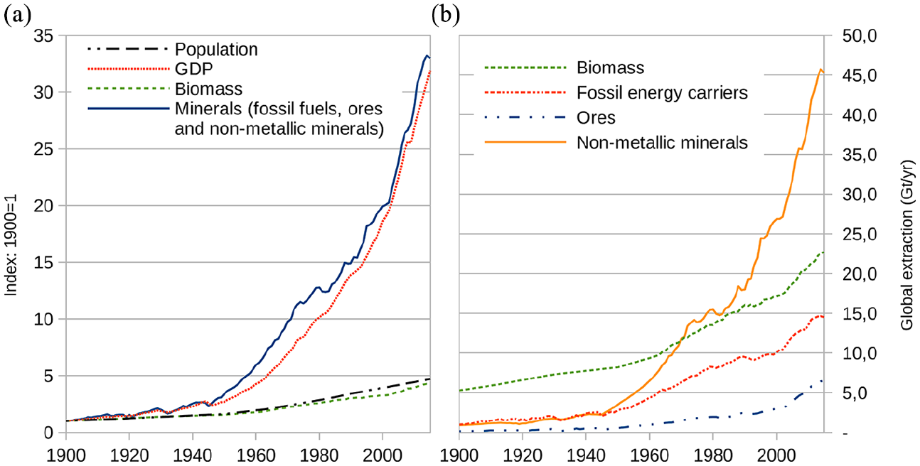
Global population, GDP and material extraction by category, 1900–2015. (a) Organic and mineral development. (b) Global extraction.
Complicating the matter, differences in environmental efficiency (GDP per environmental pressure) between countries will result in net flows of environmental factors even when the same type and volume of good is exchanged. An increasing difference in environmental efficiency between regions – or a stable difference in environmental efficiency combined with increasing volumes of trade – would, all else equal, increase trade-embedded net flows into the more efficient region. Thus, differences in consumption levels and in environmental efficiency will produce similar net flows of environmental factors, but the implications are rather different.
To date, there has been no systematic attempt to isolate and include all global studies of environmental factors in trade, independent of method or indicator (e.g. Wiedmann and Lenzen, 2018 who focus on input-output studies). In particular, no one has had attempted to identify the long-term trends of different trade-embedded environmental factors between major world regions and between developing and developed countries during the Great Acceleration. This review article aims to do precisely this, in order to shed light on the relative importance of population, affluence and environmental efficiency as determinants of the direction of flows for different indicators (cf. Fischer-Kowalski et al., 2014 on IPAT).
Method and delimitations
This is a systematic state-of-the-art review of global environmental factors in trade, focusing on long-term trends. Using primarily the search engine LUBsearch, which allows simultaneous searches of 135 subject databases and database platforms, we have identified 357 studies of global environmental factors published between 1968 and 2020. The environmental factors included as key terms were primarily adopted from previous review articles (e.g. Wiedmann, 2016) and multi-indicator studies (Arto et al., 2012; Moran et al., 2013; Wood et al., 2018), but partly expanded during the search process. Ideally, studies were retained if: 1) they present empirical estimates of actual flows; 2) these flows refer to totals of the respective embedded environmental factor, excluding studies of individual commodities or groups of commodities; 3) flows are between nation states or groups of nation states, excluding flows on subnational or municipal level, or between individual industries or industrial sectors (even when these flows are global); 4) they are ‘global’ in the sense that a significant number of countries are included with representatives from several continents.
Based on the unit of measurement studies have been grouped in eight categories that include or partially overlap with other organising principles (e.g. biogeochemical cycles, Butcher et al., 1992; planetary boundaries, Rockström et al., 2009; headline indicators, Steinmann et al., 2018). Weight-based measures were further subdivided according to the element(s) on which they were based (sulphur, phosphorous, nitrogen, carbon), with non-carbon elements (+particulate matter and non-volatile organic compounds) grouped as ‘pollutants’, and one type of carbon-based study (human appropriation of net primary production, HANPP) given its own heading (Table 1). (For bibliometric details and method, cf. Supplemental Appendix 1: A1. A complete list of the studies, their studied factors and temporal coverage, and full references can be found in Supplemental Appendix 2.)
Environmental factors, units, number of studies, temporal coverage and stylised extraction→appropriation flowchart.
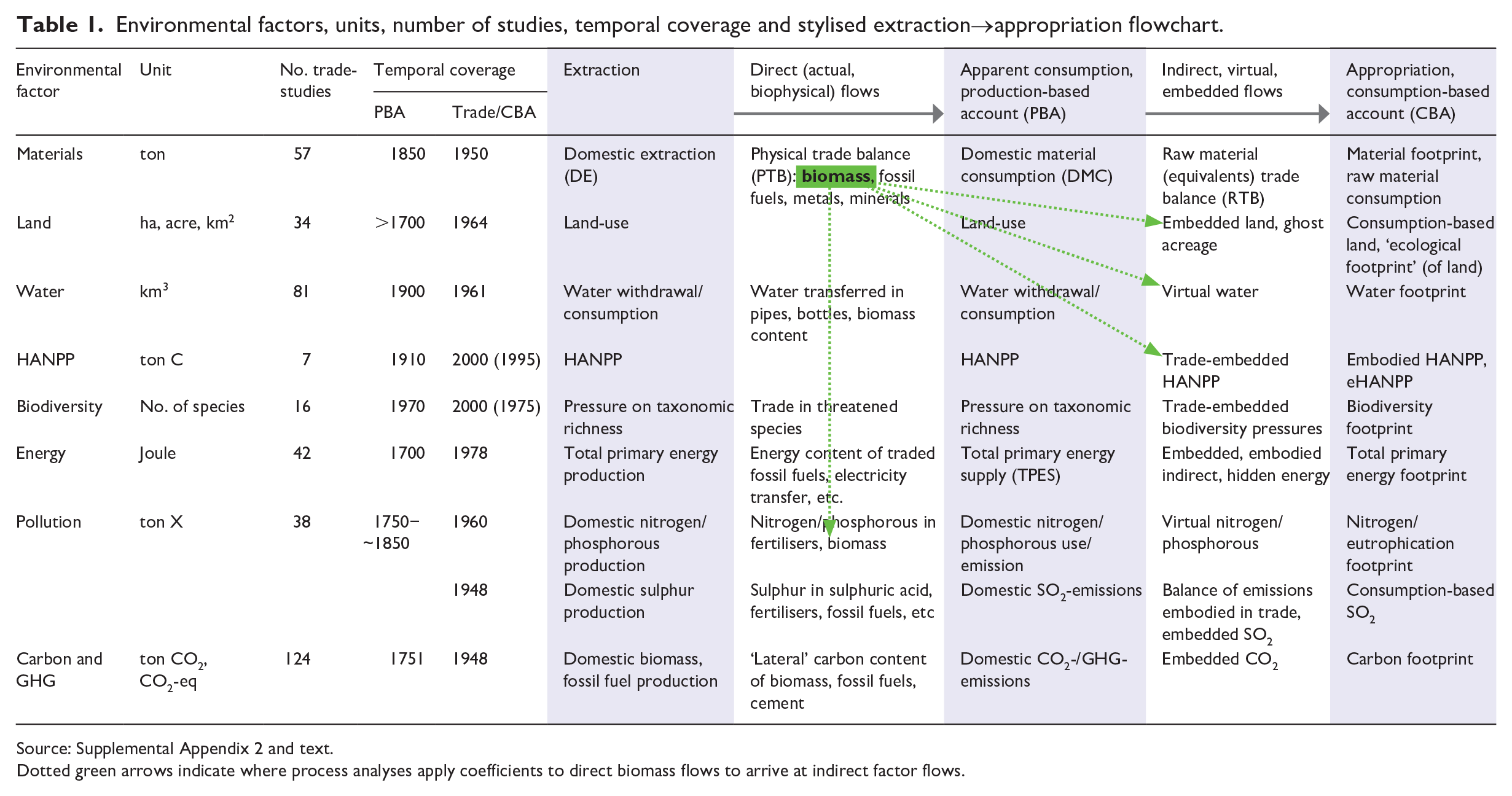
Source: Supplemental Appendix 2 and text.
Dotted green arrows indicate where process analyses apply coefficients to direct biomass flows to arrive at indirect factor flows.
For each indicator we identified the temporal coverage of environmental factor flows (Figure 3), and the discrepancy in temporal coverage between global CBA and PBA (although we have not attempted a full review of PBA) (Table 1). We focus on trade-studies with the longest temporal coverage rather than methodological sophistication and robustness. This somewhat downplays top-down (i.e. input-output) studies (and ‘indirect’ flows), since multi-regional input-output (MRIO) databases begin at best around 1990 (cf. Supplemental Appendix 1: A2), and emphasises bottom-up (i.e. process analysis) studies and ‘direct’ flows) that are commonly based on UN-data starting around 1960. Process analysis applies environmental coefficients to the physical amounts of traded goods (‘direct flows’, notably of biomass, Table 1), while MRIO traces the environmental impact of economic sectors worldwide through global monetary flows all the way to final consumers (i.e. household consumption, private investment and public expenditure). The relative merits and complementarity of these approaches have been much debated over the past decades, pointing out sectoral cut-off and an inability to distinguish between intermediate and final consumers as a problem in process analysis, and large ‘rest-of-the-world’ groups and low sectoral disaggregation in agriculture for many MRIO (e.g, Eisenmenger et al., 2016; Feng et al., 2011; Hubacek and Feng, 2016; Lenzen, 2000; Lutter et al., 2016; Piñero et al., 2018), with the principal advantage of process analysis for this review being its greater temporal coverage (Weinzettel et al., 2014).
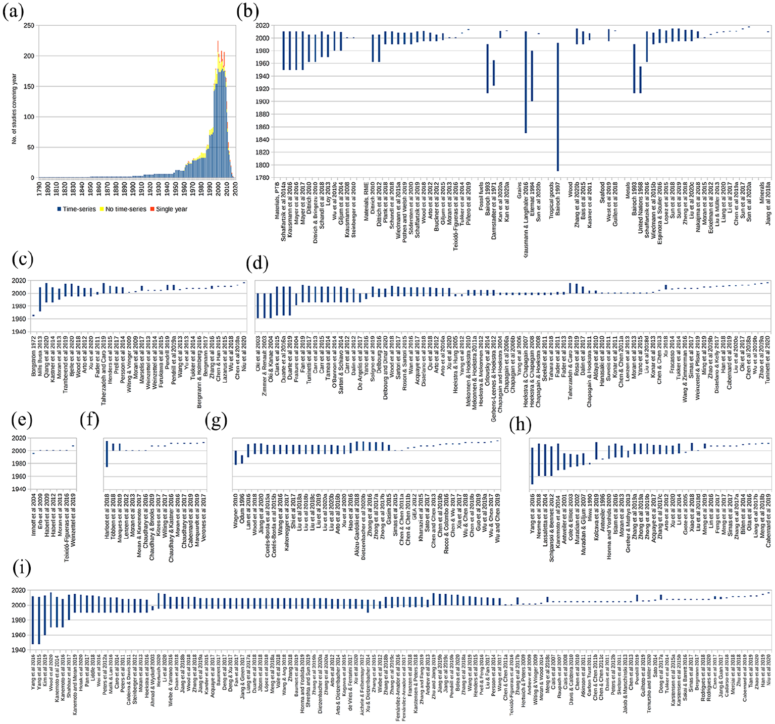
Temporal coverage in studies of environmental factors in trade. (a) Temporal coverage. (b) Materials: physical trade balance (PTB), raw material equivalents (RME) and constituent elements. (c) Land. (d) Water. (e) HANPP. (f) Biodiversity. (g) Energy. (h) Pollution. (i) Carbon/GHG. (a) Number of studies covering each year (N = 357). (b–i) Period studied by indicator.
Comparisons of trends and direction of flows draw on the above distinction between population density, affluence and environmental efficiency, but have been complicated by the fact that countries are often grouped differently among studies. For our figures we have rearranged national data, where available, into comparable groups based on the United Nations Statistics Division (UNSD) development and geographical regions, but modified for countries linked to the Former Soviet Union and Allies (FSU-A). (For country groupings, cf. Supplemental Appendix 3).
Results – global trade-embedded environmental factors
Each subsection begins with a brief description of the environmental factor and the temporal coverage in PBA and trade-studies respectively, then describes long-term trends, discusses the role of affluence, population density and/or environmental efficiency for the direction of net flows, and occasionally how differences between process analysis and MRIO may affect results.
Materials
Material flow analysis accounts (in tons) for how groups of materials – fossil fuels, biomass, ores (or metallic minerals) and non-metallic minerals (or industrial and construction minerals) – flow into, through and out of societies as part of their ‘social metabolism’ (Fischer-Kowalski et al., 2011). 2 The analysis has three layers: extraction, (apparent) consumption and appropriation (Schaffartzik et al., 2019) (Table 1). Domestic extraction (DE) is linked to domestic material consumption (DMC) via net imports of actual materials in the form of goods and commodities, that is, ‘direct flows’ (DMC=DE+Id−Ed), called the physical trade balance (PTB=Id−Ed). Domestic material consumption is linked to appropriation, the material footprint (MF), via net imports of raw material equivalents – that is, ‘indirect flows’ of materials that are used upstream (as ‘intermediates’) in the process of production but not actually transported between countries (MF=DMC+Ii−Ei) – called the raw material (equivalents) trade balance (RTB=Ii−Ei). For example, of the sharp rise in non-metallic mineral extraction during the Great Acceleration (Figure 2b) only 3% was traded directly but 33% indirectly in 2010 (Schaffartzik et al., 2019). DMC can be considered ‘production-based’ in relation to the consumption-based MF, but is simultaneously the ‘apparent consumption’ compared to extraction. Global estimates of material extraction reach back to 1850 (Krausmann et al., 2009, 2013a, 2016), but comprehensive studies of PTB begin at best in the 1950s and of RTB in the 1960s (Figures 3b and 4).
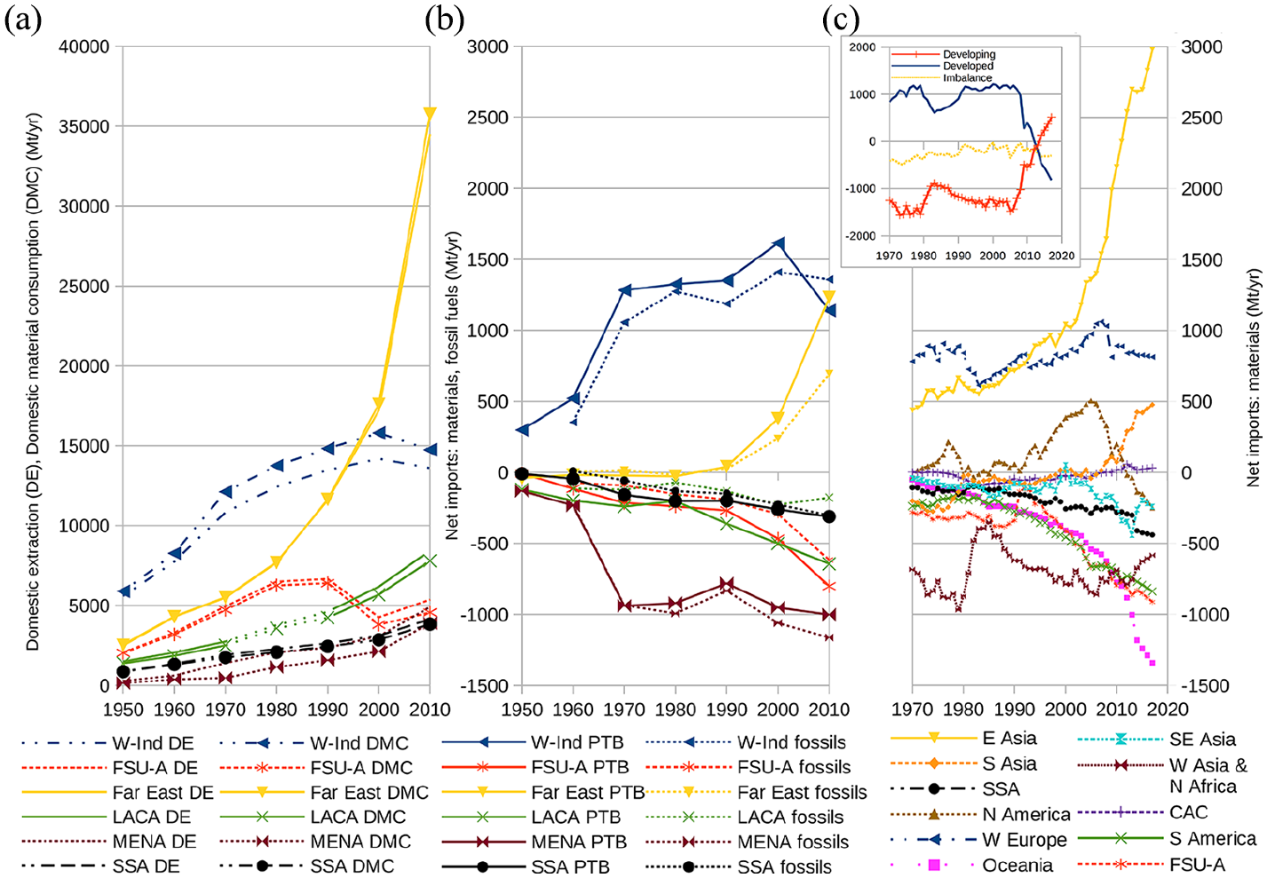
Material extraction, consumption and physical trade balance (PTB). (a) Extraction and consumption. (b) Traded materials and fuels. (c) Traded materials by UNSD group.
Several strains of global material flow estimates have culminated in the recently available global database of the United Nations Environmental Programme (UNEP, 2018) reaching back to 1970 for PTB (Figure 4c) and 1990 for RTB. However, the studies with greatest temporal coverage are all based on data from Schaffartzik et al. (2014). These estimates reach back to 1950, using UN Comtrade data until 1960/62 and stretched back in time using WTO trade statistics on the assumption ‘that aggregate physical trade flows changed with the same growth rate as monetary trade flows between 1950 and 1960’ (Schaffartzik et al., 2014: 89).
In Schaffartzik’s et al. (2014) study of direct material flows, Western Industrial countries and Asia both lead material extraction and are the only net importing regions (Figure 4). Rapidly rising Western Industrial net imports until the 1970s are wholly dominated by fossil fuels and balanced by Middle East and North African exports (Figure 4b; cf. Bairoch, 1993; Dittrich, 2010). This signals the much greater importance of fossil fuels in physical than in monetary terms (44%−57% vs 6%−17 % of merchandise exports in 1962−2018; Schaffartzik et al., 2014; World Bank, 2020b). From the 1990s Asia joins in as net importer, led by fossil fuels, tightly followed by metals and to a lesser extent biomass. Latin American net exports are intermittently headed by fossil fuels and metals, but with an increasing share of biomass since the 1990s. With the exception of biomass in 1980 and 1990, the Former Soviet Union and Allies is an overall net exporter, dominated by fossil fuels and especially after the demise of communism. Sub-Saharan Africa’s net exports are relatively small, but also dominated by fossil fuels, followed by metals, while small biomass exports turn into imports from 2000 onwards (Schaffartzik et al., 2014; Figure 4b).
Schandl et al. (2018) confirm this pattern of direct material flows into densely populated Europe and the recent increase in net imports into Asia from more sparsely populated areas like Latin America, the Former Soviet Union, Australia and Africa. This should not be interpreted as ‘developing country’ exports, since in the latest UNEP (2018) update developing countries as a group have recently become net importers. This is explained by net imports becoming increasingly dominated by Eastern Asia (while Southern and Southeastern Asia diverge as respectively net importer and exporter), by Northern America shifting from net importer to exporter, and rising net exports from Oceania (Figure 4c).
However, in terms of raw material equivalents (indirect flows) only Europe and North America remain net importers, because of the large raw material requirements for the manufactures exported from Asia+Pacific, in line with arguments on rich countries displacing environmental burdens to poor (Schaffartzik et al., 2019; Schandl et al., 2018). According to Plank et al. (2018), this recent shifting of production from efficient developed to inefficient emerging developing economies added one third to global raw material consumption over the 1990–2010 period compared with a no-trade scenario. Thus, in terms of raw material equivalents trade appears to have contributed both to environmental inequality and environmental inefficiency. However, it is not clear if the inefficiency may also have caused the inequality, since lower efficiency in natural resource use will raise the raw material equivalents embedded in a nation’s exports.
Moving back in time beyond 1950 has so far only been attempted for specific categories of goods rather than aggregate material flows (Figure 3b; including all studies that go beyond 1948 in Figure 3a). As noted, well over half of global trade in monetary terms in 1913 was in primary products, and presumably much more in physical terms. Using various estimates by Bairoch and Etemad (plus Yates, 1959) we have created a rough physical trade balance of primary products exchanged between developed and developing countries just before WWI (Table 2). Merely adding up individual net flows, sums to gross flows of ~55 Mt which is small by current standards, but compared with De Vries (2010) estimate of intercontinental trade at ~0.5 Mt in 1800, suggests an expansion by two orders of magnitude already in the course of the 19th century. Net exports of primary products from developing countries were still modest at 7.6 Mt (Table 2).
Physical trade balance (PTB) of primary products between developed and developing countries, a 1909/13 (1000 metric tonnes; negative values mean developed country net exports).
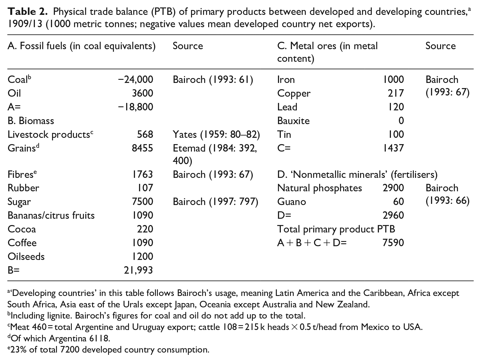
‘Developing countries’ in this table follows Bairoch’s usage, meaning Latin America and the Caribbean, Africa except South Africa, Asia east of the Urals except Japan, Oceania except Australia and New Zealand.
Including lignite. Bairoch’s figures for coal and oil do not add up to the total.
Meat 460 = total Argentine and Uruguay export; cattle 108 = 215 k heads × 0.5 t/head from Mexico to USA.
Of which Argentina 6118.
23% of total 7200 developed country consumption.
The general picture from raw material (i.e. non-foodstuff) exchange between developed and developing countries in 1909–1913 is that developed countries as a group were almost wholly self-sufficient (Bairoch, 1993). The deficit in fibres (where global trade was nevertheless dominated by US cotton exports) was more than compensated for by coal exports, especially from the UK, but also Germany, the US and even Japan (importing countries are not specified, but cf. Infante-Amate et al., 2020 and Rubio et al., 2010 on Latin America). Compared to the overwhelming role of biomass in material extraction and consumption (Figure 2b), fossil energy played a relatively much greater role in trade already at this early date – total developed country fossil fuel exports alone sums to 143.5 Mt (Bairoch, 1993: 61). Only in tropical foodstuffs – the comparative advantage par excellence of tropical countries – was global trade clearly dominated by developing country exports. The global grain trade was instead dominated by European imports from tsarist Russia and the US (Krausmann and Langthaler, 2019) – both of which flows are internal to ‘developed countries’ as defined in Table 2 – along with other regions of recent settlement such as Argentina (Infante-Amate et al., 2020), which was also relatively wealthy (Díaz-Alejandro, 1970). Europe is comparatively densely populated, and hence land scarce in relative terms, and should be expected to import agricultural goods from land-abundant frontier regions, whether tropical and poor or temperate and rich (Findlay and Lundahl, 2017). Similarly, the rice trade was mostly internal to developing countries within Asia, notably between Southeast Asian frontier areas and densely populated South and East Asian areas (Latham and Neal, 1983), a pattern suggested also by net biomass flows during the Great Acceleration (Figure 8a).
Land
Unlike materials, land cannot be traded directly, only as embedded, for example, in agricultural goods. As one of the classical economic productive factors ‘land’ has been included in many studies of factor endowments and the factor content of trade (e.g. Antweiler and Trefler, 2002; Bowen et al., 1987; Leamer, 1984). As an environmental factor it refers to flows in area-based units, accounting for the upstream land requirements of traded goods and services, distinguishing especially between agricultural, pasture and forested land. (Cf. Bruckner et al., 2015 for a review of land-based approaches, and Supplemental Appendix 1: A4 on Ecological Footprints).
Several global territorial or production-based accounts of land use are available, reaching back to 1700 or even the entire Holocene. While including elements of historical documentation, they tend to be ‘hindcasts’ (model-based predictions of past conditions) based on population estimates and sometimes very different per capita land-use assumptions (Ellis et al., 2013; Klein Goldewijk et al., 2017). By contrast, global studies of trade-embedded land – understood as area-based environmental indicators – are limited to the most recent decades (Figure 3c).
Conclusions on the direction of flows of embedded land vacillate between emphasising affluence (land flows from poor to rich regions) or natural endowments/population density (from land-abundant to land-scarce regions) as determinants. Occasionally, different environmental efficiencies across the globe are added to the blend. Thus, Wilting and Vringer (2009) explain net imports for most developed countries by less efficiently produced imports (meaning that more land per unit of agricultural good will be embedded in imports than in exports), in addition to negative trade balances (greater volumes imported) and structural specialisation (more land requiring types of goods imported, e.g. beef).
Comparisons between studies are complicated by the fact that countries are grouped differently among them. Moran et al. (2013) find that while exports of lower income countries had higher land intensity (land/$), the larger volume of less land-intensive exports from high-income countries nevertheless make them net exporters of land in absolute terms. Dorninger and Hornborg (2015) dispute this conclusion, but refer only to EU, US and Japanese imports rather than to Moran’s et al. entire high-income group (Moran et al., 2015). In Arto et al. (2012) the EU, the US and Japan are also major net importers over the 1995–2008 period, while India, China and even Russia (all BRIC countries except Brazil), shifted from net exporters to importers. Wood et al. (2018) find that the OECD countries increased their net imports of land over the whole 1995–2011 period. Net imports were dominated by Europe in 1995, but by 2011 China had caught up, pointing to population density as an explanatory factor in addition to a certain level of income. The major net exporters were South America, Russia, Australia and Africa+Middle East – all parts of the world with a low population density. Prell et al. (2017) find that rich countries tend to be net importers of land and more central in the trade network, while China and India are also central but (here) instead net exporters. Conversely, countries with larger land endowments per capita are more likely to become net exporters of land and remain peripheral in the network. Bergmann and Holmberg (2016) treat capital investments as the final consumption and find strong net transfers of land from developing to developed countries, with endowments and scarcity playing lesser roles (cf. Södersten et al., 2020). In Chen et al. (2018) land-rich countries (e.g. Australia) and/or less-developed economies (e.g. Africa) export to densely populated countries (China) and/or to more-developed economies (EU, Japan and US). Tukker et al. (2014) favour population density/endowments as explanations of net flows, while Yu et al. (2013) emphasise affluence and indirectly power relations, although simultaneously pointing to land-rich Brazil, Russia and Australia as suppliers of land-demanding goods globally, and believing that populous China and India are likely to increase their imports as they get richer. Both Weinzettel et al. (2013) and Wang et al. (2013) associate land exports with high domestic biocapacity (biomass productivity), whereas domestic income conditions the geography of imports and footprints of consumption.
Many have pointed to differing results depending on methodology (Hubacek and Feng, 2016; Kastner et al., 2014b; Moran et al., 2009; Schaffartzik et al., 2015; Wiedmann, 2009). Process analyses apply land-coefficients directly to volumes of traded (biomass-based) goods (Kastner et al., 2014a), but exclude land-based inputs into traded manufactures and services (Weinzettel et al., 2014), with results lying closer to the apparent consumption of biomass. MRIO allocate land-use to the monetary output of different sectors and trace the land embedded in that output through monetary transactions between nations and sectors to its appropriation by final consumers (Arto et al., 2012; Bjelle et al., 2020; Moran et al., 2013; Wood et al., 2018). It is therefore even more telling when top-down studies also find patterns conforming to those expected from comparative advantage based on population density.
Kastner et al. (2014a) apply land-coefficients to biomass flows, focusing on cropland and major animal products. They find regional characteristics to be fairly stable over the 1986–2009 period (Figure 5a: bottom): Western Europe, Eastern Asia, Central America and the Caribbean and Northern Africa and Western Asia were major net importers. Northern America, Oceania and increasingly South America were major net exporters. Sub-Saharan Africa, Southern Asia and Southeast Asia were more balanced, and the Former Soviet Union and Allies shifted from being net importers in 1986 to net exporters in 2009. These trends and patterns, which conform well with Borgström’s (1972) estimate for 1964–66, also closely follow those for biomass and nitrogen (Figure 8), and resemble those for virtual water (Figure 6). They suggest that land flows from areas with low to high population density per grazing land and cropland, a specialisation according to endowments that may have been accentuated for example with the trade-openings between Western Europe and the Former Soviet Union and Allies in the 1990s. Contrary to the affluence perspective, developing countries increasingly become net importers (Figure 5a: top).
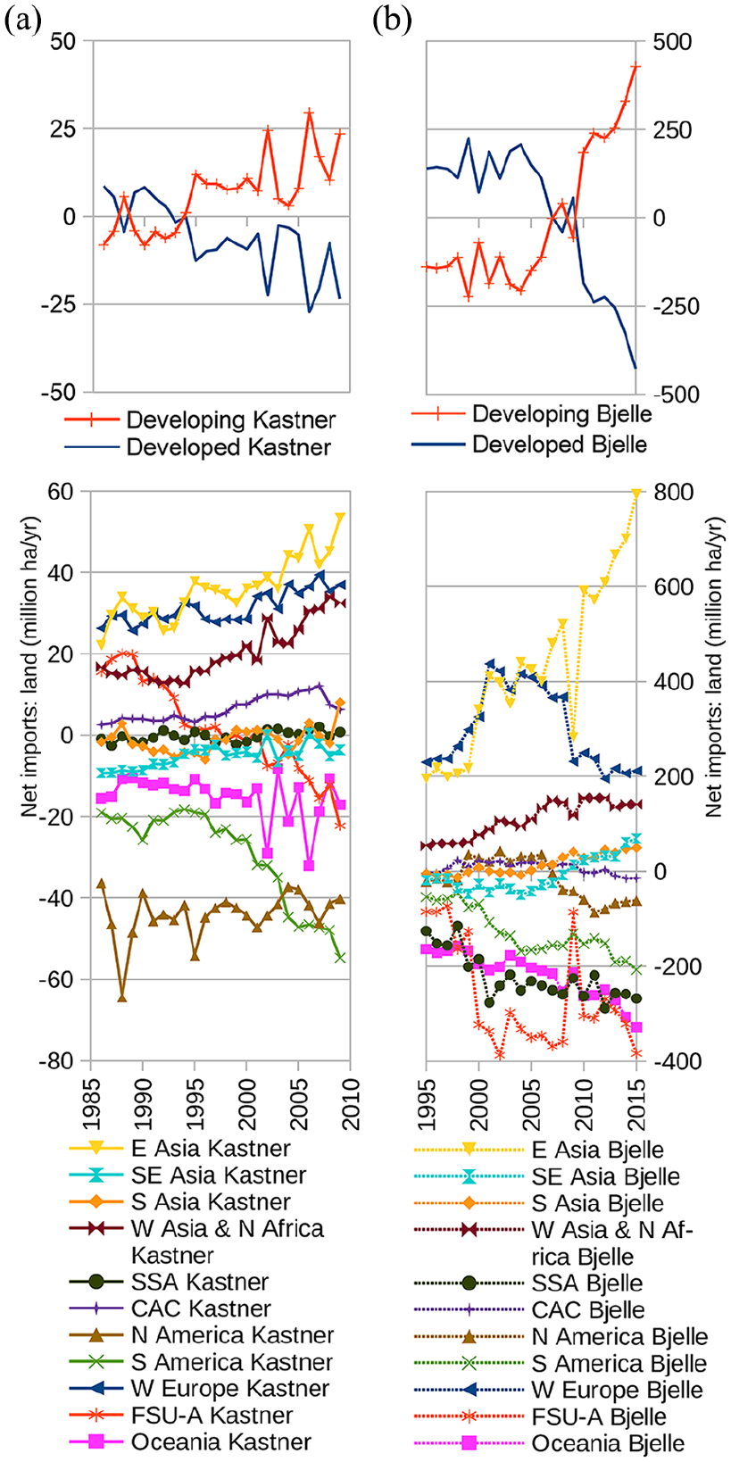
Trade-embedded land. (a) Biomass-based. (b) MRIO-based.
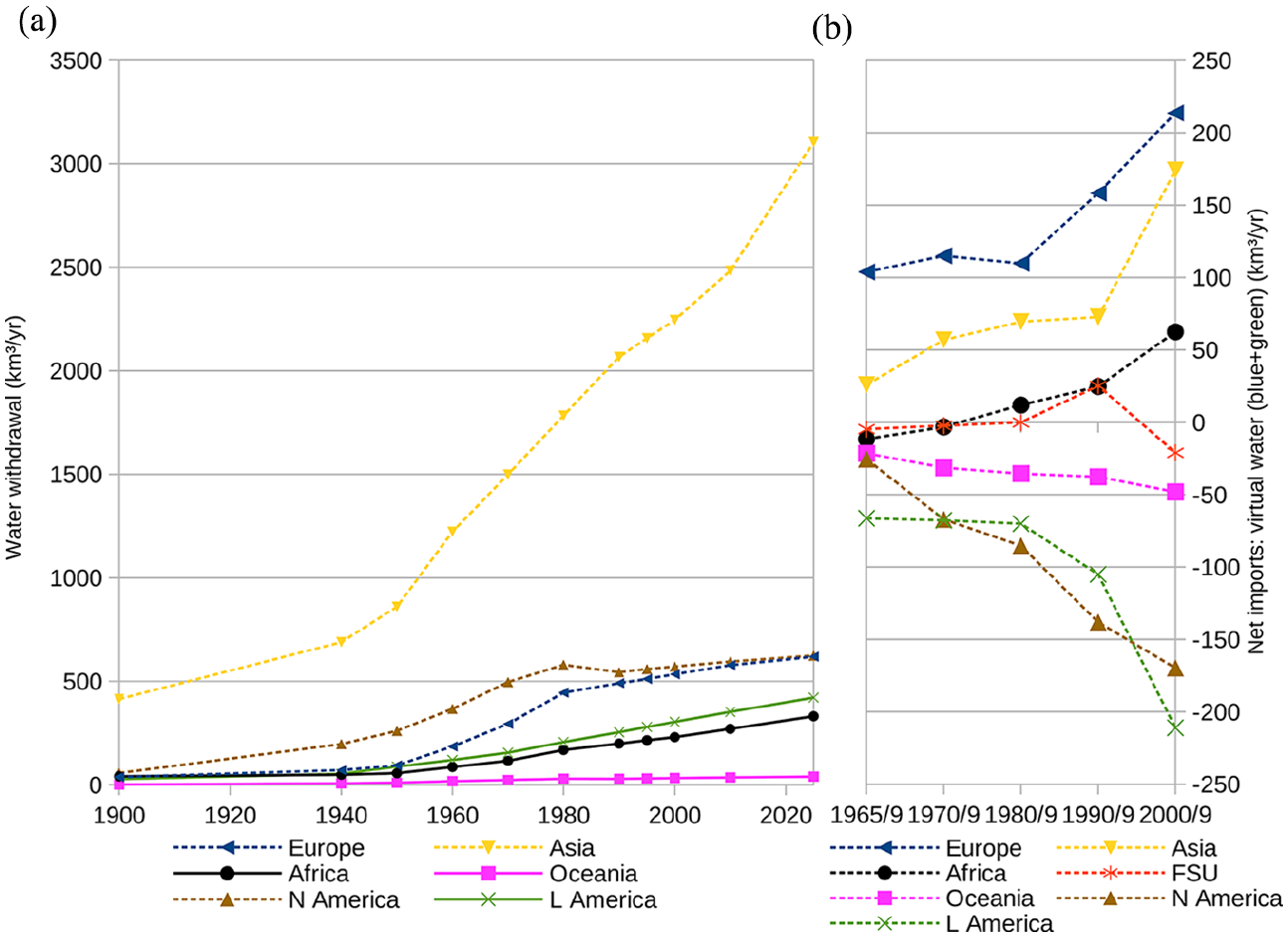
Water withdrawal and virtual water trade. (a) Water withdrawal. (b) Virtual water.
In the MRIO-based estimates for 1995–2015 by Bjelle et al. (2020) trade-embedded land flows are up to an order of magnitude higher – notably including also forest products (timber, paper, etc) and land-based goods used as input in manufacturing and service sectors and thereby embedded in their output – but otherwise show some similarities between regions: Western Europe, Eastern Asia, Western Asia and Northern Africa are the greatest net importers, Oceania and South America are great net exporters, while Central America and the Caribbean, Southern and Southeastern Asia also show trends similar to those in Kastner et al. (2014a). However, in Bjelle et al. (2020), the Former Soviet Union and Allies is a more prominent net exporter, and the shift towards developing countries becoming net importers occur only around 2010 – that is, after most other MRIO-studies break of – mostly because of Asian developments, but also because of a drop Western European net imports and Northern America (here) only then becoming a net exporter. The greatest difference nevertheless concerns the increasingly prominent net exports of Sub-Saharan Africa (Figure 5b). By contrast, in Kastner et al. (2014a), Sub-Saharan Africa was a net importer of biomass, although due to its low agricultural yields became about balanced in terms of land. It is unclear how much of these relative differences is explained by including trade in forest and non-biomass products.
Overall, even in studies that otherwise emphasise affluence, numerous exceptions that support endowments/population density can be found. From a theoretical point of view, the comparative advantage of high-yielding, land-rich countries would presumably cause global supply to become increasingly concentrated to a few large net exporters. In addition, the low income elasticity of demand for food in Engel’s Law (Engel, 1857) suggests that agricultural goods and environmental indicators that rely heavily on them should be more equal in demand per capita, affecting net flows to follow population density – provided that you have at least the barest means of subsistence (cf. Davis, 2001; Marselis et al., 2017; Satya, 1997), and allowing for a one-time shift to a more dairy- and meat-based diet with higher income. If so, income differentials would rather play out in other, mineral-economy indicators that more reflect rising demand for manufactures and services, although these would still embody biomass as raw materials and other inputs.
Water
Freshwater is connected to land via the catchment area. Its appropriation by humans has implications not only for the viability of human societies but also for ecosystems (Rockström et al., 2009; Schyns et al., 2019). Household consumption and direct trade are Lilliputian compared to ‘virtual’ water use and trade. Virtual water refers to the amount of freshwater that is used in the production of goods or services, primarily in agriculture, but also, for instance in electricity generation from hydropower or nuclear power (for cooling). Its most voluminous constituent is ‘green’ water, stemming from precipitation that is stored in the root zone of the soil and evaporated, transpired or incorporated by plants. ‘Blue’ water is sourced from surface or groundwater resources, and ‘grey’ water is the amount of fresh water required to assimilate pollutants (D’Odorico et al., 2019; ‘scarce’ water is derived from blue water; e.g. Lenzen et al., 2013).
Territorial estimates of global water consumption and withdrawal by continent and sector (i.e. agriculture vs industry) go back to 1900, when agriculture’s share (dominated by wet-rice cultivation of monsoon Asia) was as high as 98% of water consumption and 91% of water withdrawal (Duarte et al., 2014; Shiklomanov and Rodda, 2003; Figure 6a). Industry’s low share (0.8% and 6.5% respectively in 1900) does not include the water embedded in raw material inputs, for example, the cotton used to produce textiles. Most global studies of virtual-water trade cover only single years or 5- to 10-year averages, but MRIO studies reach back to 1995, network studies to 1986 and on agricultural goods to 1965 or 1961 (Figure 3d).
Several papers have found that ever since 1961 much water is saved globally from trade compared to what would have been needed without it (Chapagain et al., 2006; Dalin et al., 2012; De Fraiture et al., 2004; Fader et al., 2011; Konar et al., 2011, 2013; Oki and Kanae, 2004; Oki et al., 2003; Soligno et al., 2019; Yang et al., 2006). Process analyses based on agricultural products show net flows between regions increasing from 1965 to 2010, mostly from Latin and North America and Oceania, to Europe, Asia and Africa, that is, from regions where population density is low (and/or water abundant) to regions where it is high (and/or water scarce) (Figure 6b; Carr et al., 2013; Dalin et al., 2012; Duarte et al., 2016, 2019; cf. Figure 5).
However, as was suggested for land, in many top-down MRIO studies developed countries stand out as net importers. Thus, whereas bottom-up studies like Duarte et al. (2016) find the US to be the world’s largest net exporter of (77.2−187.6=) −110.4 km3 of virtual water in 2010, Arto et al. (2016a, using MRIO) find the US to be the world’s second largest net importer of (419.6−249.2=) 170.4 km3 in 2008. The discrepancy is particularly vast for imports (77.2 km3 compared to 419.6 km3). Both studies apparently use the same agricultural conversion factors from the Water Footprint Network (e.g. Mekonnen and Hoekstra, 2010, 2011a), but Arto et al. (2016a) also include industrial goods and grey water, including evaporation from hydroelectricity plants (Gentry et al., 2012; Mekonnen and Hoekstra, 2011b). The difference is nevertheless striking. In the Water Footprint Network’s own (bottom-up) estimate for 1996–2005 the US is still a net exporter of (234.1−313.7=) −79.6 km3 when industrial sectors and grey water is included, or (167.1−257.7=) −90.7 km3 if not (Hoekstra and Mekonnen, 2012). The explanation, according to Feng et al. (2011) and Wang and Zimmerman (2016), is that the water in US agricultural exports recorded in bottom-up approaches, returns in top-down approaches – like the proverbial evil spirit – as even greater inputs in industrial imports.
HANPP
Human Appropriation of Net Primary Production (HANPP) is an estimate of human impact on and extraction of plant-based biomass, or more technically, on the flow of trophic energy (‘biomass’) in ecosystems, namely the net primary production (NPP) which is the basis of plant growth and thus, in turn, potentially available as food for other species (Haberl et al., 2014). HANPP consists of two parts. First, HANPPharv is the biomass derived carbon or energy directly and indirectly appropriated by human societies through harvests. Second, HANPPluc is the sum of productivity changes resulting from land use and land conversion. Much as in studies of the global carbon budget (e.g. Ruddiman et al., 2016), it corresponds to the difference between potential net primary production, NPPpot (a theoretical construct of global NPP without any human land-use), and actual net primary production, NPPact. Thus, HANPP=HANPPharv+HANPPluc, where HANPPluc=NPPpot−NPPact.
Territorial HANPP has been estimated to double globally from 6.9 GtC/year in 1910 to 14.8 Gt C/year in 2005, or from 13% to 25% of potential NPP, although still leaving non-human nature’s share constant in absolute terms (Krausmann et al., 2013b, Supplemental Appendix 1: A6). Global studies of trade-embedded HANPP mostly refer to the year 2000 (Figure 3e, Supplemental Appendix 1: A6). According to Haberl et al. (2014) international trade flows amounted to 1.7 Gt C/year, or about a tenth of total HANPP. They went predominantly from sparsely populated regions in the Americas and Oceania to densely populated regions in Europe and East Asia, seemingly independent of development or income status (cf. Erb et al., 2009; Haberl et al., 2009, 2012; Moran et al., 2013), although Weinzettel et al. (2019) suggest a bias towards affluent imports. Teixidó-Figueras et al. (2016) conclude that consumption-based so-called eHANPP is more equally distributed than territorial HANPP, so that trade plays a directly equalising role.
Biodiversity
Biodiversity refers to the taxonomic richness (genetic variability, number, abundance and distribution of species, genera, etc.) of a geographic area (Swingland, 2013). Trade-embedded pressure on biodiversity is commonly measured in number of threatened species. The Living Planet Index exemplifies a global territorial estimate of loss of vertebrate populations, reaching back to 1970 (WWF, 2018). Unfortunately, longer-term estimates of anthropogenic extinction rates vary by orders of magnitude, much depending on whether they are global modelling efforts or long-term regional studies. Some suggest increased rates of vertebrate extinction since the late 19th century (Li et al., 2016) and drastically rising rates of extinction (up to 1000 times or more) above background rates for the past 200 years (Ceballos et al., 2015; McRae et al., 2017; Newbold et al., 2015). Others find much variation but no net trend in biodiversity (Dornelas et al., 2014; Ellis et al., 2012; Vellend et al., 2013, 2017). Decreased global biodiversity is still compatible with overall stability or increase on regional scales, since the same species may contribute to biodiversity in different locales.
This section treats only the indirect effects of trade on biodiversity when, for instance, cash crops for export replace wildlife, rather than the inadvertent transfer of invasive species or direct trade in threatened species (Harfoot et al., 2018). Apart from Marques et al. (2019) and Többen et al. (2018), all global studies of trade-embedded biodiversity threats refer to single years between 2000 and 2012 (Figure 3f). The estimated share of threats related to trade in relation to the total biodiversity threats range between 17% and 30% (Chaudhary and Kastner, 2016; Chaudhary et al., 2016; Kitzes et al., 2017; Lenzen et al., 2012), with Marques et al. (2019) seeing a rising trend from 2000 to 2011. Lenzen et al. (2012) concluded that developed countries tend to have low exports of biodiversity threats, possibly because of greater environmental protection (or already fewer species). Major net importers are found in North America, the EU and East Asia. Conversely, major supply chains originate in developing countries that are rich in biodiversity and with export-oriented agricultural, fishing and forestry industries, notably in South and Southeast Asia and Africa, but also Russia (Lenzen et al., 2012). That developed countries exert large biodiversity impact in developing countries is corroborated by Chaudhary et al. (2016), Chaudhary and Kastner (2016), Kitzes et al. (2017), Moran and Kanemoto (2017), Wilting et al. (2017) and Marques et al. (2019), who find that the per capita consumption impact in North America, Europe and the Middle East is an order of magnitude greater than the production impact, although it decreased over time in the Americas, Africa and Western Europe and increased in Eastern Europe, the Middle East and Asia and the Pacific. The perspective changes somewhat in Verones’s et al. (2017) attempt to advance from ‘pressure’ to ‘impact’ indicators. Estimating the damage on species diversity through climate change, terrestrial acidification, eutrophication, land and water stress, they find that although wealthy countries displace ‘pressures’ (embedded land, water, CO2) to lower-income countries, their ‘impacts’ (on species variety) instead tend to originate in high-income countries. Lower income countries also exert most of their impact in their own income category. Többen’s et al. (2018) physical-monetary hybrid approach will benefit from the recent country extension of land-use in EXIOBASE (Bjelle et al., 2020).
Energy
Numerous proposals coexist on how to evaluate energy’s direct and indirect contribution to nature and society, including as a common ‘currency’ for both ecology and economy based in global insolation (Hau and Bakshi, 2004; Sciubba, 2010, Supplemental Appendix 1: A7). Most energy accounting is more concerned with understanding society’s energy requirements at different levels of development, and starts instead where energy enters the economy (Kander et al., 2013; Warr et al., 2010).
Primary energy production/extraction is linked to the total primary energy supply (TPES) via trade in primary energy (coal, crude oil and natural gas) and secondary or final energy (refined oil products and electricity crossing borders in transnational nets) – that is, direct energy flows. TPES is linked to the energy footprint via indirect (embedded/embodied) energy flows – mainly in the form of energy-intensive bulk commodities (e.g. aluminium, steel) and products for final consumption (fertiliser, steel rails, cars, clothes). Current energy accounting reports only direct energy flows traded between nations, whereas embedded energy trade is not reported systematically (Akizu-Gardoki et al., 2020; GEA, 2012). Global production-based accounts for fossil and biomass energy reach back to between 1700 and 1850 (Court, 2016; Etemad and Luciani, 1991; Fernandes et al., 2007; Fouquet, 2016; Smil, 2017), although detailed long-term national studies are scarce (Supplemental Appendix 1: A7). Global studies of direct flows go back to 1925 or 1913 (Table 2), but embedded energy studies only to 1978 or, with time series, 1995 (Figure 3g).
GEA (2012) estimates gross direct energy trade flows in 2005 between nine world regions to some 190 EJ (Exajoules, 1018 Joules) and gross embedded energy flows to another 100 EJ. Thus, at least half of total primary energy supply (500 EJ) was traded between these regions either directly or indirectly. Naturally, net flows are smaller. The EU, the US and Japan dominate both direct and indirect imports, while China and the rest of Asia stand out as being simultaneously importers of direct energy and large exporters of indirect energy (Figure 7), resembling the pattern observed for direct and indirect material flows (Schandl et al., 2018).
Trade-embedded energy.
Direct flows after 1950 were dominated by rapidly rising Middle Eastern exports to the industrial West (including Japan) until the 1970s, and rapidly rising Asian imports and Former Soviet Union exports since the 1990s (Figure 4b). The plateauing of Western Industrial direct energy imports since the oil crises of the 1970s may have been followed instead by growing imports of indirect or embedded energy. This is suggested by Wagner’s (2010) finding that the ratio of embedded flows to direct flows grows in line with GDP per capita for the 1978–2000 period. Lan et al. (2016) also conclude that the share of energy footprints in imports increases with per capita GDP over the period 1990 to 2010. Arto et al. (2016b) find that net embedded energy exports from emerging developing to developed countries increased from 13.5 EJ in 1995 to 29 EJ in 2008, or from 6.6% to 13.8% of developed countries’ energy consumption. These developments may be interpreted as an outsourcing of the energy footprint – a continued but ‘hidden’ increase in energy consumption (Akizu-Gardoki et al., 2020) – but may partly result from an increasing energy efficiency of domestic production compared with that of one’s trading partners (Baumert et al., 2019).
The situation of large amounts of embedded energy exports going hand in hand with large manufacturing exports is not new, and resembles the situation for the UK in the period 1832–1935. The difference is that the UK (and developed countries in general) during this first phase of globalisation also exported direct energy (Table 2, Brolin and Kander, 2020; Kander et al., 2017).
Pollutants
Here, ‘pollutants’ include heterogeneous indicators such as nitrogen (N), phosphorous (P), both N and P plus potassium (NPK), nitrous and nitrogen oxides (N2O, NOX), sulphur oxides (SOX), particulate matter, ozone precursors and more (Figure 3h). For convenience, these have been grouped into a) studies of eutrophying (mostly agricultural) macronutrients (measured in tons of N and/or P) and b) studies of airborne (mostly industrial) emissions, where we concentrate on sulphur dioxide (measured in tons of SO2). (For studies that convert greenhouse gases into CO2-equivalents cf. section ‘Carbon and greenhouse gases’).
Eutrophication
Most nitrogen on Earth is in the form of atmospheric N2, but studies of nitrogen in trade concern all its other forms, so called ‘reactive nitrogen’ revolutionised by the Haber-Bosch process for nitrogen fixation in 1913 (Galloway and Cowling, 2002). Phosphorous is almost always found as phosphate (PO43−), mostly in rocks and currently mined primarily in Morocco, USA and China. Phosphorous is the main hazard in freshwater and nitrogen in marine eutrophication (Laws, 2018; low iron concentrations limit nitrogen fixation in seawater). Both are in the high-risk zone of Rockström’s et al. (2009) planetary boundaries.
Global estimates of the fixation and extraction of nitrogen and phosphorous and/or their agricultural use go back into the 19th century (Lu and Tian, 2017; Smil, 1990; Steffen et al., 2015; Vitousek, 1994; Xu et al., 2019). However, national detail is limited before FAO series start in 1961, which is also the limit for the most extensive trade studies for direct phosphorous (Nesme et al., 2018; Schipanski and Bennett, 2012) and nitrogen flows (Lassaletta et al., 2014). These studies concern the nutrients contained within traded food and feed products themselves, rather than the ‘virtual’ nitrogen or phosphorous leaked or emitted in the process of producing agricultural and industrial goods. Studies of global virtual nitrogen and phosphorous flows start at best in 2000 (Hamilton et al., 2018; Oita et al., 2016; cf. Shibata’s et al., 2017 for a review).
For estimates based on the nitrogen and phosphorous (protein) content of the same agricultural goods, trends and directions of flows should be similar. And indeed, direct flows of both increased eightfold between 1961 and 2010–2011: nitrogen from 3.0 to 23.6 Mt N/year (Lassaletta et al., 2014) and phosphorous from 0.4 to 3.0 Mt P/year (Nesme et al., 2018), compared with the 11 Mt P/year traded in 2011 as mineral fertiliser. In both instances, cereals, soybeans and feed for animals dominated the increase. Schipanski and Bennett (2012) point out that phosphorous exports appear to be concentrated in regions with greater fertiliser use efficiencies (i.e. naturally rich soils) in line with the theory of comparative advantage, although they warn that this could hide depletion of more fertile soils in countries such as Argentina.
The story is much the same for direct nitrogen flows, where the regional pattern reminds of those for biomass and land (Figure 8), with a few highly net-exporting countries – in 2010 the United States, Argentina and Brazil were responsible for more than 11 Mt – and many increasingly net-importing countries. Oceania, Northern America and eastern South America are net exporters. Europe, Africa and Western Asia, western Latin America and the Caribbean, Eastern and recently Southeastern Asia are net importers. India has shifted from importer to exporter, and the Former Soviet Union and Allies shifted from being an exporter in 1961 to becoming a large importer in 1986, but was back as an exporter again by 2010 (Figure 8b, Lassaletta et al., 2014).
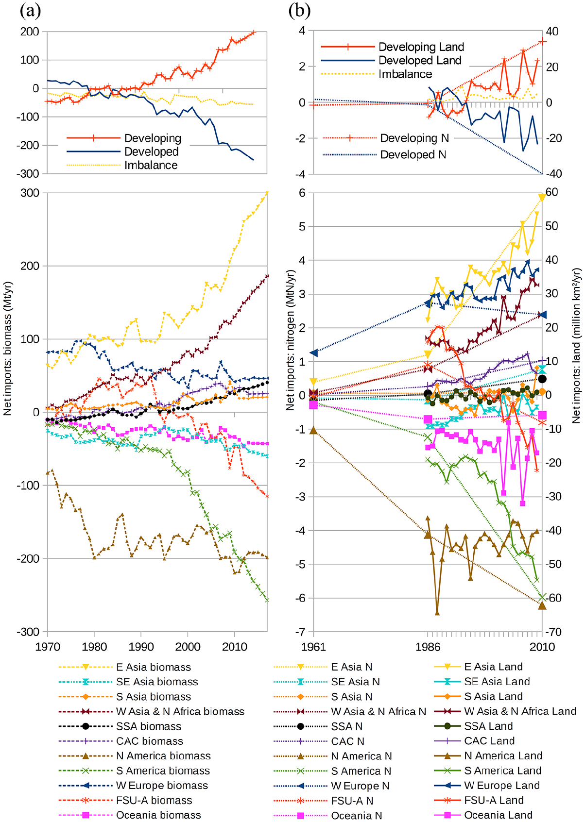
Trade-embedded biomass, nitrogen and land (superimposed). (a) Physical trade balance: biomass. (b) Trade-embedded nitrogen and land.
In Oita’s et al. (2016) estimate for 2010, virtual nitrogen embedded in trade is almost twice as high (41.8 Mt) as direct flows (23.6 Mt) or roughly a quarter of total agricultural and industrial emissions. Major net exporters tend to have significant agricultural, food and textile exports and include China, Australia, Pakistan, India, Argentina, New Zealand and several developing economies, whereas important net importers are the major high-income economies in East Asia, Western Europe and the US, followed by Russia and Mexico (Oita et al., 2016). In Hamilton et al. (2018) manufactures and services contribute more than a third of all trade-embedded eutrophication potential and high-income countries similarly emerge more clearly as major importers.
Air pollution
Air pollutants have long been of concern for their effects on human and ecosystem health (Fowler et al., 2020; Tiwary et al., 2019). Territorial estimates of airborne polluting emissions go back to 1750 (Hoesly et al., 2018) or ~1850 (e.g. Bond et al., 2007; Höhne et al., 2011; Ito and Penner, 2005; Lamarque et al., 2010; Smith et al., 2011; Figure 9a). We shall focus on trade-embedded SO2 emissions – of concern as an aerosol and source of acid rain.
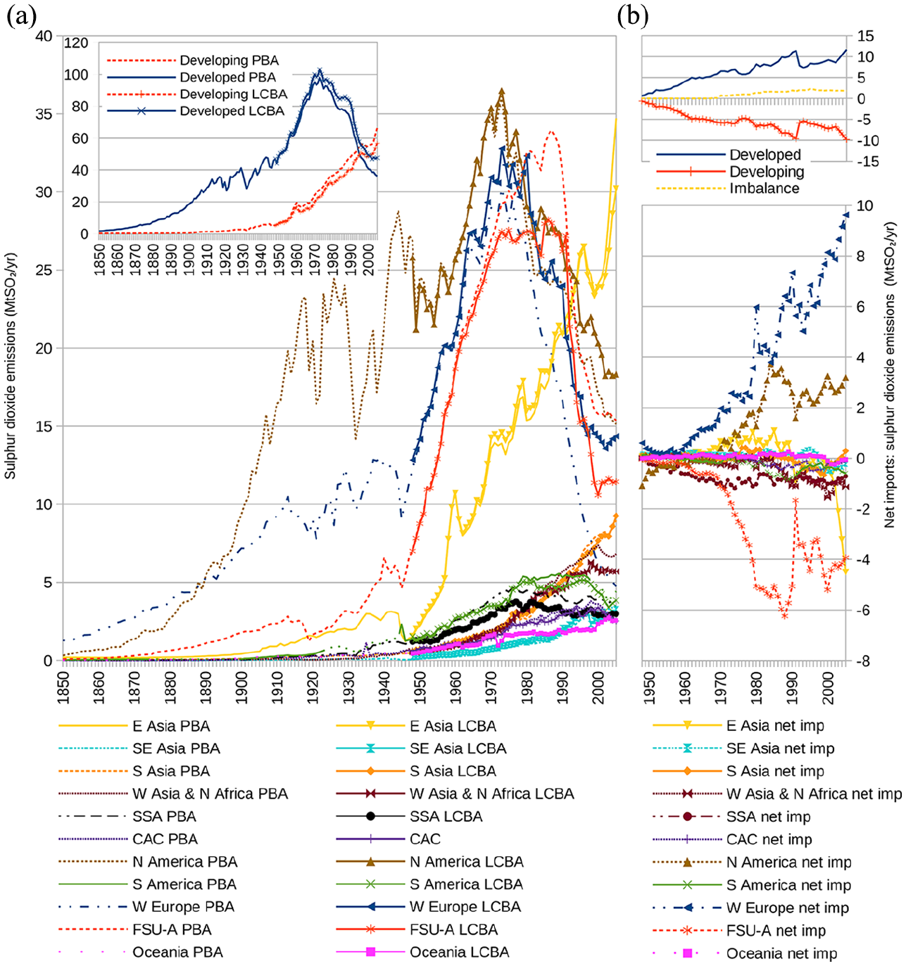
Total and trade-embedded SO2 emissions. (a) So2-emissions. (b) Trade-embedded SO2.
While the studies included here concern SO2-emissions, sulphur is also used and traded directly, mostly as sulphuric acid and fertiliser. Total consumption increased from 1.4 Mt in 1901 to 59.3 Mt in 2000, and 76.4 Mt by 2011, with traded direct flows rising from 15 Mt in 1981 to 21 Mt in 2000 and 28.3 Mt by 2009 (Kutney, 2013; Messick, 2011; Ober, 2002). Starting in 1958, most of this sulphur was recovered from fossil fuels, and by lowering the sulphur content or sulphur:carbon ratio of fuels largely makes up for the difference between SO2- and CO2-emissions trajectories (Figures 9a and 10a).
The most extensive global studies of trade-embedded SO2-emissions go back to 1970 using MRIO (Kanemoto et al., 2014), and to 1948 using a more simplified approach (Long-term Consumption-Based Account, LCBA) that aggregates all national sectors and commodities into one sector (Yang et al., 2015: 795, 2016). Using data from Yang et al. (2016) and Smith et al. (2011, including emissions from fossil fuels, industrial processes, and biomass burning), the net flows of embedded SO2 for major world regions in 1948–2005 can be reconstructed (Figure 9b, Supplemental Appendix 1: A8). Large increases in net imports into Western Europe and to some extent Northern America can be found. These correspond to net exports from the Former Soviet Union and Allies and, increasingly since the 1990s, Eastern Asia, where Chinese net exports were responsible for 7 Mt in 2005 or more than 100%. Latin America and Oceania, which figure prominently in indicators related to agricultural exports, play minor roles in embedded SO2, while Western Asia and Africa here are net exporters. The pattern in 2005 resembles that for embedded energy (Figure 7), suggesting that trade volumes play a larger role at this time and regional scale than differences in sulphur:energy ratios.
The debate on trade-embedded pollution has been dominated by the idea of ‘pollution havens’, where dirty industrial production is located globally to countries that have slacker environmental regulations. The shorter atmospheric life and local or regional environmental effects of SO2, compared with the long atmospheric lifetime and global consequences of CO2, suggest a reason why environmental regulation and outsourcing should play a larger role for SO2 (Cole and Elliott, 2003; cf. Muradian et al., 2002). Arguing against the idea, the low cost of regulations, mostly under 4% of total production costs, means that they had only marginal effect on plant location decisions and trade flows (Copeland and Taylor, 2004). Kanemoto et al. (2014) argue that burden shifting is real in that developed country net imports began earlier for pollutants than for greenhouse gases and link this to a series of environmental regulations in the developed nations. Yang et al. (2016) also find transfers from developing to developed countries to start earlier (Figure 9b) and the ratio of transferred to total emissions to be higher for NO2, CH4 and SO2 than for CO2. Grether and Mathys (2013) find a rising trend of SO2-emissions embedded in trade in 1990–2000 (consistently >15% of total emissions) in spite of declining emission coefficients (i.e. more but cleaner goods were traded). The US, East Asian and West European high-income countries were the largest importers of pollution generating goods, while China, followed by Chile, Indonesia and Mexico were the most significant exporters. On average, emission intensities of high income countries were higher in imports than in exports, suggesting support for the pollution haven argument (Grether and Mathys, 2013).
Still, this does not prove that outsourcing of pollution intensive industries from developed to developing countries takes place, only that the developing countries have on average more polluting technologies (Jakob and Marschinski, 2013). If developing countries use less efficient technologies in exports than do developed countries, this increases their net outward flows, but does not necessarily imply that they suffer pollution effects or a detrimental burden shifting as a consequence of international trade (as argued by Muradian et al., 2002). If they had satisfied domestic consumption with their own more emission intensive technologies their pollution situation could very well have been equally bad or worse than without the international exchange.
Long-term production- and consumption-based SO2-emissions both follow an inverted-U curve for developed countries with a turning-point around 1970, but only around 1990 for the Former Soviet Union and Allies (Figure 9a). By contrast, in developing countries, lead by Eastern and to a lesser extent Southern Asia – in line with the shifting centre of world GDP and manufacturing (Amsden, 2001; Baldwin, 2016; Crafts and Venables, 2001; O’Rourke and Williamson, 2017) – they continued to rise throughout the Great Acceleration. Thus, the large net-flows in Figure 9b could result from rapid environmental efficiency improvements in Western Europe and North America, and lagging improvements, first in the Former Soviet Union and Allies and then in Asia (e.g. the continued use of coal with high levels of sulphur). This implies a link between net emissions exports and a trade surplus in manufactures together with low environmental efficiency (e.g. coal based technologies and high territorial emissions). The same reasoning suggests that during 19th century industrialisation the coal-using developed countries would also have been net exporters of trade-embedded air-pollutants, but to date there are no such studies even on a national scale.
Carbon and greenhouse gases
Carbon dioxide is the principal agent in climate change and ocean acidification (IPCC, 2013; Rockström et al., 2009). Global estimates of territorial CO2 emissions from fossil fuels and cement reach back to 1751 (Boden et al., 2017), from biomass burning to 1900 or more (Marlon et al., 2008; Mieville et al., 2010; Mouillot et al., 2006), and, still much debated, from land-use for the entire Holocene (e.g. Klein Goldewijk et al., 2017; Ruddiman et al., 2016). Estimates of greenhouse gas emissions reach back to 1750 (Hoesly et al., 2018) or 1850 (Gütschow et al., 2016, 2017). Disregarding land-use, the cumulative climate impact from developed and developing countries respectively has been estimated since 1850 (Wei et al., 2012).
While concern is over emissions, carbon is also traded directly as biomass or fossil fuels, in which case the CO2 is eventually released in the importing country and becomes part of its production-based emission statistics (Table 1). Studies of direct carbon are limited to the year 2004 (Ciais et al., 2007, 2008; Davis et al., 2011; Peters et al., 2012), but could easily be extended using material flow data.
Global trade-embedded CO2 (or CO2-equivalents when speaking of greenhouse gases in general) start with production-based estimates of sectoral CO2-emissions that are assumed to virtually accompany output throughout the production process until it is appropriated as household consumption, business investments, or public expenditure (Table 1). Normally, carbon contained in biomass, for example forests, is treated as neutral with respect to CO2 emissions, but this only holds true if the regrowth of forests equals what is cut down. Currently this appears roughly to hold true on a global scale, with temperate net reforestation compensating somewhat for tropical net deforestation (Jia et al., 2019). A few studies estimate the trade-embedded carbon or CO2 released by tropical deforestation (Henders et al., 2015; Pendrill et al., 2019), whereas others examine the link between the ‘forest transition’, re- and afforestation and the associated CO2-uptake to trade-embedded displacement of deforestation (Kastner et al 2011; Li et al., 2017; Meyfroidt et al., 2010, 2013; Mills Busa, 2013).
Most studies – all top-down – cover only CO2 originating in fossil fuels (and cement) after 1990, and are concerned with the possible trade-embedded carbon leakage between developed and developing countries (or more precisely between Annex I and non-Annex I countries of the Kyoto protocol). Peters et al. (2011) even suggest that all the emission reductions accomplished by the developed countries in response to the Kyoto protocol were offset up by outsourcing polluting production to less developed countries. By contrast, Kander et al. (2015), Jiborn et al. (2018), Baumert (2017), Baumert et al. (2019) and Zhang (2018) find that in the period 1995–2009 most of what seemed to be outsourcing was in fact due to technology differences between developed and developing countries. Thus, they were not due to a specialisation pattern in the world where the developing countries take on more energy intense production like steel, pulp and chemicals and leave the lighter industrial production and services to the developed countries. When technologies are globally normalised for each product group, there is no longer a clear divide in the world between developed and developing nations. Certain developed countries, mainly the US and UK, do outsource, while EU 27 as a unit does not. China insources, that is, specialises somewhat in energy demanding heavy industrial production, but a substantial part of their virtual carbon exports is due to their coal-based energy system and their monetary trade surplus. So far, there are no studies of technology-normalised flows before 1995.
The studies by Kanemoto et al. (2014, 2016) and Yang et al. (2015, 2016), starting in 1970 and 1948 respectively, all find increasing shares of trade-embedded net flows from developing to developed countries at least since the 1980s (Figure 10b: top). Reconstructing Yang’s et al. (2016) trade-embedded CO2 from their published LCBA has been complicated by uncertainties regarding their PBA data after 1980 (Supplemental Appendix 1: A8). Disaggregating by region (Figure 10b: bottom), it appears that Western European net imports started rising from around 1970 and Northern American net imports in the 1980s, but as for SO2 corresponding to increased exports from the Former Soviet Union and Allies. Similarly with SO2 and energy, Oceania was also a net importer. While net exports rise persistently from most other regions (as for developing countries in general), these only took off with Eastern Asian (Chinese) net exports in the 2000s. Again, this suggests outsourcing primarily to an environmentally inefficient Soviet bloc specialising in heavy industry, while developments since the 1990s could be explained by a combination of technological inefficiency and outsourcing to China, in line with the conclusions from the normalised technology studies for 1995–2009.
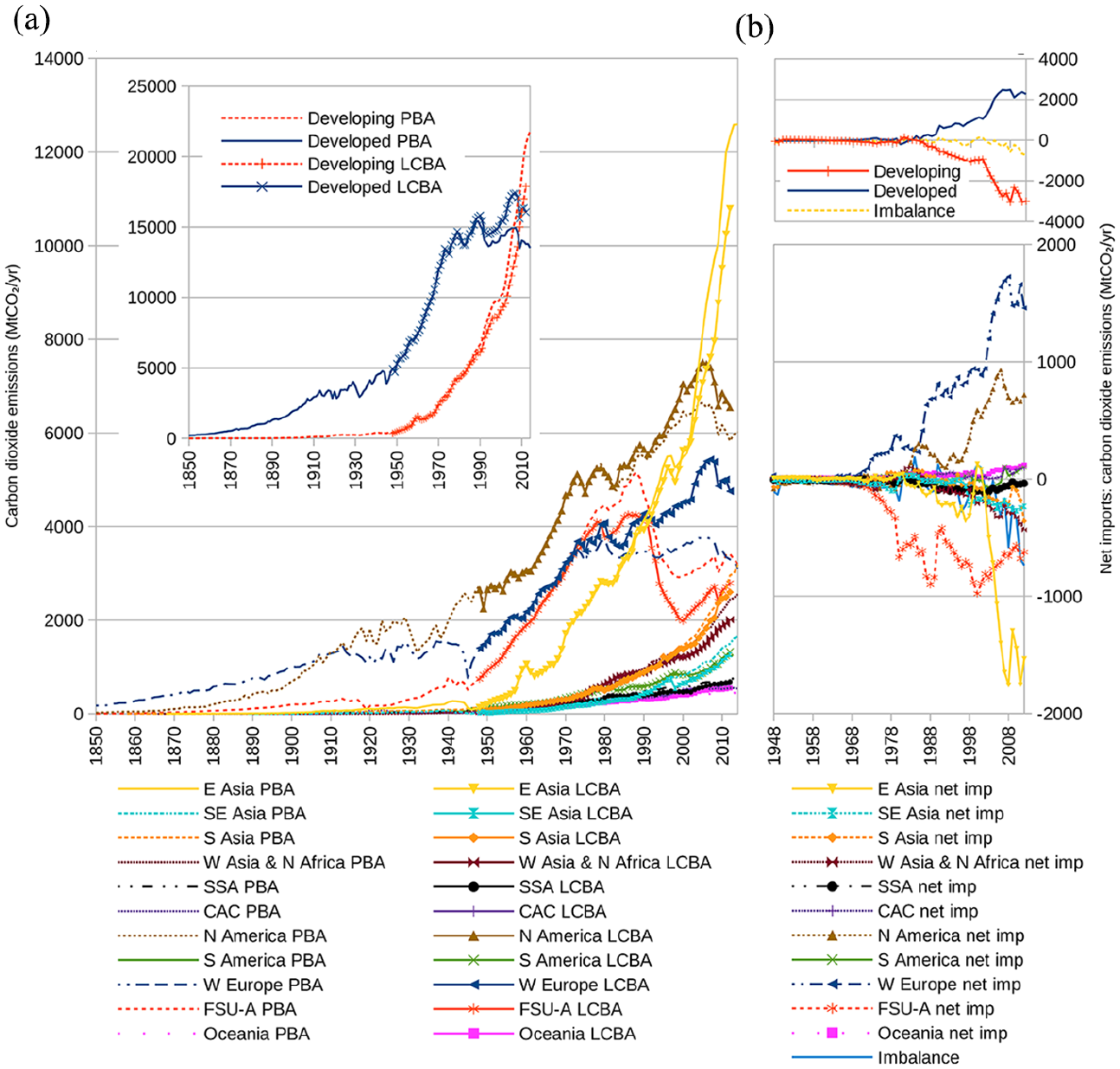
Total and trade-embedded CO2 emissions. (a) CO2-emissions. (b) Trade-embedded CO2.
Recently, net flows from developing to developed countries appear to have plateaued (Pan et al., 2017) or peaked (Wood et al., 2020), due to stagnating Chinese exports and decreasing emission intensity. This implies a smaller role for carbon leakage in the future, but also reflects the increasing share of South–South trade, which by 2014 was equal to North–North trade (Fouquin and Hugot, 2016, https://ourworldindata.org/grapher/share-of-world-merchandise-trade-by-type-of-trade), and shifts in the global supply chain towards other regions of the global south (Jiang and Green, 2017; Jiang et al., 2018; Wiedmann and Lenzen, 2018). Many studies conclude that both the reduction of total emissions and of net exports from developing countries would be best achieved by low-carbon technology development in and transfer from developed countries (Hotak et al., 2020; Li et al., 2020), although so far foreign direct investment has rather been associated with higher developing country emissions (Essandoh et al., 2020).
Efficiency gains notwithstanding, unlike for SO2 there has been no absolute decline in emissions, and both production- and consumption based CO2-emissions still trail the shifts in economic growth – the rise of Eastern Asia, Western European and Northern American slowdown in the 1970s and 1980s, the collapse of the Soviet bloc, the aftermath of global financial crisis in 2008–2009 (Figure 10a). Overall, CO2 emissions are still closely related to economic development (affluence), but trade-embedded emissions also reflect trade-balance (mostly in manufactures) and relative environmental efficiency.
Discussion – the raison d’être of Great Acceleration factor flows
Our review confirms the view of a Great Acceleration in trade-embedded factor flows after 1950, but their rates and direction differ over time and depending on indicator – notably whether they reflect an ‘organic’ or ‘mineral’ economy.
A recurring theme has been net transfers between developed and developing countries, with affluence as the driving force. However, indicators that depend heavily on trade in biomass (i.e. land, water, HANPP, direct flows of phosphorous and nitrogen) point to a concentration of net exports to a few highly productive and land-abundant countries in line with theories of comparative advantage, whereas imports are determined primarily by population density and only secondarily by affluence. This is in line with our initial expectations from Engel’s law (Engel, 1857) that consumers spend proportionally less of their income on basic necessities such as food and clothing as income increases, and from Krausmann’s (2015) observation that population growth drives global biomass consumption and GDP drives fossil fuel and mineral use (cf. Krausmann et al., 2009; McNeill and Engelke, 2014). In other words, global inequalities of income are not as much reflected in indicators dominated by biomass and agricultural goods as they are in indicators where minerals, fossil energy, industrial goods and services play a larger role. This difference is discernable even among different methodologies studying the same indicator. Thus, by environmentally extending direct flows of biomass, process analyses downplays (relative to MRIO) factors embedded in the output of downstream sectors (e.g. manufactures) and thereby final (compared to intermediate) consumer appropriation, which is the focus of MRIO.
Nevertheless, by the same measure, environmental factor flows related to minerals and fossil energy may indeed be more closely related to a developed–developing country income differential. Here, there is a kind of etherialisation at play from direct to indirect flows. Coal was still cumbersome to transport and therefore had more domestic linkages, ending up produced in and exported from the most developed 19th-century economies. From the 1950s, net imports of direct material flows and energy – largely Middle Eastern oil – into Western developed countries increased rapidly until the 1970s. They then stagnated as higher energy prices stimulated both greater production and technological efficiency within the developed countries themselves. At the same time, affluent countries started becoming net importers of indirect flows relating to the mineral energy economy.
The shift of world manufacturing to low-wage developing countries, especially in Asia over the past half century (Amsden, 2001; O’Rourke and Williamson, 2017; World Bank, 2020a), has greatly influenced environmental factor flows as reflected in the rise of direct imports to and indirect exports from Asia. Thus, the most significant changes in direct material flows since the 1980s concern rising Asian imports and the exports of their suppliers. Simultaneously, net exports from Asia and net imports into developed countries increased for indirect flows such as Raw Material Equivalents, embedded energy and emissions. The fact that this rise began earlier for locally polluting emissions such as SO2 than for CO2 suggests an impact from environmental regulations, but it is partly explained by the profitability of recovering sulphur for other usages and a shift away from coal, which instead has increasingly fuelled Eastern and Southern Asian economic growth. While Asian countries have increasingly turned into centres for intermediate, ‘apparent’ consumption for the appropriation of affluent developed countries, there is no indication that this has been detrimental to their own affluence or that of their suppliers (Muradian et al., 2012).
However, while these indirect flows conform to the traditional developed–developing country divide, they could in principle be equally well explained by the third leg of the IPAT identity: technological differences in environmental efficiency. The observation that until 1990 Western net imports of SO2 and CO2 were balanced by net exports from the Former Soviet Union and Allies rather than the traditional developing countries of Africa, Asia, or Latin America, suggests outsourcing to heavy industry in the Soviet bloc and that environmental efficiency was a more important element. Studies for 1995–2009 using normalised technology suggest that outsourcing of emissions was more important in the US and the UK, but not for the EU as a group, and that insourcing was important for China. Thus, the drivers of these trends are not as simple as world specialisation.
Yet, since the technology frontier tends to lie in high-income countries, with a 50-year lag before transferring to lower-income countries (Allen, 2012), poorer technologies, also in environmental terms, will become the ‘comparative advantage’ of poorer countries. This ‘indirect’ income effect via technology may be the principal cause of net factor flows also from poor to rich – yet another head on the ‘Maxwellian demons’ on the borders of rich countries that we inherit from the century preceding the Great Acceleration.
Conclusion – a plea for time
If we wish to understand the patterns of development during the Great Acceleration we should also study their origins and possible path dependencies. Unfortunately, our limited knowledge about global environmental factor flows before 1950 is immediately apparent from our review – contrasting with global production-based accounts that commonly extend back to ~1850. Global process analyses rely on UN data that start around 1960, while the prohibitive data requirements of global MRIO tables makes going beyond 1970 – the current record by extrapolation (Kanemoto et al., 2014, 2016) – a possibly insuperable task. Yang et al. (2015, 2016) propose their shortcut model specifically to address this problem, although its robustness still needs further testing. Similarly to material flows, the starting date in 1948 is set by the easy accessibility of WTO trade data from that year.
How then, can our knowledge be pushed beyond 1950? Brolin and Kander (2020) consider the option of spreading the coverage of long-term studies of regions and goods until they add up to a global picture. Another option would be to start with long-term global PBA data and allocate them according to trade-embedded flows and CBA, by environmentally extending global trade statistics that have recently been made more accessible (Dedinger and Girard, 2017; Federico and Tena-Junguito, 2016).
Benchmark estimates of 19th and early 20th century intercontinental trade in monetary terms can be found, for example, in Hanson (1980), Lewis (1981), or Bairoch and Etemad (1985), who also report the commodity structure of Third World exports. Paying greater attention to intra-Asian trade, Sugihara (2015) about doubles Asian volumes. Although this update has yet to be incorporated, especially two recently released databases with annual estimates offer great prospects, at least from the 1860s onwards when coverage is more complete. First, the open-source database RICardo (Dedinger and Girard, 2017, http://ricardo.medialab.sciences-po.fr), which took 12 years to develop citing 1300 sources, contains bilateral trade data for an increasing number of entities (not always countries) over the period 1800–1938. Second, the related Federico-Tena database (Federico and Tena-Junguito, 2016) contains the full value of imports and exports for most countries in the world, both in current and constant prices, and their underlying data allow the analysis of product groups for several countries.
A more time demanding possibility is to revisit the original sources cited in these and other works to complement monetary with physical trade balances. These could then serve as a starting point also for other bottom-up or hybrid approaches, for example using contemporary land or energy coefficients (cf. Aguilera et al., 2015; Kander et al., 2017; Theodoridis, 2017; Warde, 2016). Unfortunately, current territorial estimates of global land-use for 1850 vary between 17.7 and 29.4 million km2 (Klein Goldewijk et al., 2017: 948), which implies very different trajectories for the 1850–1950 period and very different coefficients (however, cf. Widgren, 2018, http://pastglobalchanges.org/ini/wg/landcover6k [accessed 4 February 2019], Stephens et al., 2019). Estimates of Europe’s trade-embedded energy in 1870–1935 (Kander et al., 2017) could be applied to air pollutants, and have already been extended to ecological footprints (Theodoridis et al., 2018). These estimates use process analysis (Bullard et al., 1978) to determine the energy requirements of goods, which may be difficult on a global scale. Instead, coefficients derived from long-term national studies or regional studies of specific commodities may have to be used as proxies for world average production technologies and technologies could be normalised. This way the structure of historical trade with regards to environmental factors can be analysed. Technology differences among nations can be discussed but more at an ad hoc basis, when data is available for individual nations and regions.
If pre-1950 global estimates of trade-embedded flows can indeed be achieved, we still need to determine for what purpose. Yang et al. (2016) argue that the dwindling difference between PBA and CBA the further back in time we go makes extensions beyond 1948 unnecessary. Cumulative emissions of CO2 transferred from developing to developed countries during the period 1948–2012 were about 36 Gt, with only around 8% of that amount taking place between 1948 and 1990, about as much as during a single year in the period 2005–2012. According to Yang et al. (2016: 474), then, ‘since trade volumes before 1948 were much smaller than current volumes, earlier transferred emissions can be safely assumed to be negligible’ and PBA be used as substitutes for CBA. Indeed, Wei et al. (2016) found that the cumulative transfer of CO2 from developing to developed countries made an almost negligible contribution to climate change compared with total emissions even in 1990–2005. Thus, for some research questions empirical extensions beyond 1948 may indeed be unnecessary. For other issues, however, this conclusion is premature.
First, while the volume of trade was smaller before 1950 (Figure 1a), several reasons can be advanced why environmental factor flows could still have been relatively important. For example, the efficiency in land, energy and resource use was often significantly lower in the past, meaning that the coefficients used to calculate embedded flows would be correspondingly higher (cf. Supplemental Appendix 1: A7). Thus, trade-embedded flows would not decrease as much as traded volumes in the past. Also, since much of the trade increase during the Great Acceleration involves shipping back and forth of the same material inputs, with some value added to it in each production step – the ‘second unbundling’ of production and consumption (Baldwin, 2016) – this suggests that the outsourcing of environmental problems would be greater relative to the volume of trade during the 19th century ‘first unbundling’, when producers and consumers were first separated globally. In addition, global trade was at a low point at the end of WWII, both relative to global production and sometimes also in absolute terms compared with the period before WWI. For Maddison (2006: 362) merchandise exports as a share of GDP grew worldwide from around 1% in 1820 to 8−9% in 1913 and 1929, but then fell to about 5% after WWII, recovering to former levels only by the 1970s. For Klasing and Milionis (2014) even this underestimates trade’s collapse with WWI: exports rose from 9% in 1870 to 15% in 1913, before dropping to 6.5 % by 1939. After WWII it fluctuated around 10%, and the 1913 level was not surpassed until 1974, continuing to rise to about 25% by 2000 (Figure 1b), which is very similar to estimated shares of trade-embedded to total environmental impact (Wiedmann, 2016). From a trade perspective, the Great Acceleration rather appears as a continuation of the trend before the world wars, the Spanish Flu and the Great Depression, and is partly a matter of catching up to former levels, at least in relation to world production.
Furthermore, questions about when current trends began and about the direction of environmental factor flows will affect our interpretations and understanding of the Anthropocene, especially since its suggested origins coincide with distinct periods of agricultural or industrial globalisation. The conclusion that flows were insignificant before 1948 stands in contrast to a vast, albeit more narrative literature (e.g. Bunker, 1985; Hornborg and Martinez-Alier, 2016; Pomeranz, 2000; Studnicki-Gizbert and Schecter, 2010) emphasising the importance of centre-periphery trade-embedded flows for colonial exploitation, the industrial revolution, the Great Divergence, as well as the characterisation of the Anthropocene. Thus, even if true, the conclusion would have to be verified in actual empirical studies and in confrontation with claims and observations from these other traditions.
For example, the Columbian Exchange in 1492–1800 is often interpreted in terms of a centre-periphery dichotomy. However, while inaugurating a globalised farming culture, trade volumes were probably too small to have had significant consequences for the redistribution of environmental burdens. Instead, intercontinental trade’s impact consisted primarily in the redistribution of species, including crops, diseases and people. Similarly, the first globalising wave of the Industrial Revolution in 1800–1914/1950 is commonly interpreted in terms of an exchange of primary products for manufactures, associated respectively with a poor periphery and a rich centre. However, while this globalisation wave can be distinguished from the foregoing era by increasing volumes of trade in both manufactures and bulk goods, it was in fact dominated by the exchange of some primary products for other primary products. This was mostly true also for trade between rich and poor countries, in 1909/13 characterised by the exchange of coal for tropical goods and largely balanced in material terms (Table 2). World trade may well have been dominated by the exchange of staple crops and fibres but this was exchanged preferably among developed and developing countries respectively, notably European grain imports from temperate and fairly affluent regions of settlement and tsarist Russia, and Southeast Asian rice exports to South and East Asia. Some of the current patterns for flows of biomass-related indicators between land-rich and land-poor countries, appear to have been created during this trade-induced great specialisation in the century before the Great Acceleration.
While we tend to assume that net flows went from developing to developed countries, in the 19th century, flows related to the mineral economy could even have been reversed. Just as recent developments are dominated by the rise of China as a factory of the world, so pre-1950 flows were dictated by the UK’s and other industrialised nations’ place as the workshop and coal-mine of the world. Long-term studies of the UK show that while it imported land intensive goods, it was indeed a net exporter of materials, ecological footprints and both direct and embedded energy (cf. Brolin and Kander, 2020; Kander et al., 2017; Schandl and Schulz, 2002; Theodoridis et al., 2018). Studies of the US show that it was a net exporter of materials, including both biomass and fossil energy (Gierlinger and Krausmann, 2012; Tilley, 2006).
There may thus be good reason to believe that also the first industrial globalisation wave shifted environmental burdens geographically, although not necessarily in the same direction as after 1950 or primarily between developed and developing countries. In general, conclusions based solely on recent data risk placing emphasis on the wrong variables and may prove unable to properly contextualise and clarify major historical shifts. Our key conclusion in this respect is the need for more systematic historical studies.
Supplemental Material
sj-pdf-1-anr-10.1177_2053019620973711 – Supplemental material for Global trade in the Anthropocene: A review of trends and direction of environmental factor flows during the Great Acceleration
Supplemental material, sj-pdf-1-anr-10.1177_2053019620973711 for Global trade in the Anthropocene: A review of trends and direction of environmental factor flows during the Great Acceleration by John Brolin and Astrid Kander in The Anthropocene Review
Footnotes
Acknowledgements
We would like to thank Anna Missiaia, Erik Green and two anonymous reviewers for useful comments that much improved the manuscript.
Declaration of conflicting interests
The author(s) declared no potential conflicts of interest with respect to the research, authorship, and/or publication of this article.
Funding
The author(s) disclosed receipt of the following financial support for the research, authorship, and/or publication of this article: Open access funding provided by Lund University.
Supplemental material
Supplemental material for this article is available online.
Notes
References
Supplementary Material
Please find the following supplemental material available below.
For Open Access articles published under a Creative Commons License, all supplemental material carries the same license as the article it is associated with.
For non-Open Access articles published, all supplemental material carries a non-exclusive license, and permission requests for re-use of supplemental material or any part of supplemental material shall be sent directly to the copyright owner as specified in the copyright notice associated with the article.