Sage Journals: Discover world-class research

Abstract

Background:

To improve efficacy, therapeutic drug monitoring is often used in clozapine therapy. Trough level monitoring is regular, but trough levels provide limited information about the pharmacokinetics of clozapine and exposure in time. The area under the concentration time curve (AUC) is generally valued as better marker of drug exposure in time but calculating AUC needs multiple sampling. An alternative approach is a limited sampling scheme in combination with a population pharmacokinetic model meant for Bayesian forecasting. Furthermore, multiple venepunctions can be a burden for the patient, whereas collecting samples by means of dried blood spot (DBS) sampling can facilitate AUC-monitoring, making it more patient friendly.

Objective:

Development of a population pharmacokinetic model and limited sampling strategy for estimating AUC_0-12h (a twice-daily dosage regimen) and AUC_0-24h (a once-daily dosage regimen) of clozapine, using a combination of results from venepunctions and DBS sampling.

Method:

From 15 schizophrenia patients, plasma and DBS samples were obtained before administration and 2, 4, 6, and 8 h after clozapine intake. MwPharm^® pharmacokinetic software was used to parameterize a population pharmacokinetic model and calculate limited sampling schemes.

Results:

A three-point sampling strategy with samples at 2, 6, and 8 h after clozapine intake gave the best estimation of the clozapine AUC_0-12h and at 4, 10, and 11 h for the AUC_0-24h. For clinical practice, however, a two-point sampling strategy with sampling points at 2 and 6 h was sufficient to estimate AUC_0-12h and at 4 and 11 h for AUC_0-24h.

Conclusion:

A pharmacokinetic model with a two–time point limited sampling strategy meant for Bayesian forecasting using DBS sampling gives a better prediction of the clozapine exposure in time, expressed as AUC, compared to trough level monitoring. This limited sampling strategy might therefore provide a more accurate prediction of effectiveness and occurrence of side effects compared to trough level monitoring. The use of DBS samples also makes the collection of clozapine samples easier and wider applicable.

Keywords

clozapine dried blood spot limited sampling strategy pharmacokinetics population pharmacokinetic model therapeutic drug monitoring

Introduction

Clozapine is an atypical, second-generation, antipsychotic drug that is proven effective for the treatment of patients with schizophrenia who are refractory or intolerant to treatment with other antipsychotic drugs.^1,2 Most patients are prescribed clozapine in a one- or twice-daily dosing regimen.³ To avoid toxic adverse effects like seizures and delirium and to optimize treatment efficacy, therapeutic drug monitoring (TDM) is often used to guide clozapine therapy.^4
–7 TDM of clozapine is particularly useful when a patient is newly prescribed clozapine, when there is poor response, by presumption of intoxication, by suspicion of poor adherence, in case of infections, in case of drug–drug interactions, by changes in caffeine intake and when a patient stops or starts smoking.^5,8,9

Between patients, large inter-individual variation in clozapine plasma levels is reported when equal dosages of clozapine are prescribed.¹⁰ Differences in plasma concentrations between patients are mainly caused by differences in bioavailability of the drug and rate of metabolism of clozapine by Cytochrome P450 (CYP) Iso-enzymes, especially CYP1A2.¹¹

In daily practice, TDM of clozapine is performed by trough level monitoring using a venipuncture. Clozapine trough levels between 350 and 700 mg/L^12
–14 are marked as therapeutic, but some patients also show clinical response on levels below 350 mg/L or above 700 mg/L.¹⁴ Clozapine plasma levels more than 1000 mg/L are considered toxic.^12
–14

Although clozapine trough level monitoring is common in daily practice, trough levels provide only limited information about the absorption and distribution of clozapine within the day. Variations in pharmacokinetics (PKs), often resulting in a significant difference in the effects of a drug, are considered a key contributor to medication efficacy.¹⁵ Drug response is therefore not only related to the clozapine trough level but depends on the exposure in time.¹⁶ The area under the concentration time curve (AUC) is a commonly used marker to estimate drug exposure in time and might therefore be a better predictor of clozapine response.¹⁵

AUC is usually calculated by means of a full PK profile over 12–24 h consisting of usually eight or more blood samples. Collection of so many samples over such a long time period is impractical, patient unfriendly, and given the costs, not a realistic option in clinical practice. Also, for research purposes, collecting many venous blood samples is time-consuming and stressful for patients. This makes it difficult to properly study the relationship between clozapine AUC and clinical response and determine whether the AUC is a better predictor of clozapine response compared to trough level monitoring.

A limited sampling strategy (LSS) meant for Bayesian forecasting may help to overcome these problems. Using this method, a limited number of samples is collected at predefined sampling times that gives the optimal estimation of the AUC using a formula or PK software equipped with a population PK model. In order to keep the method patient friendly, the number of samples is usually limited to a maximum of three.^15,17

A method to make TDM of clozapine more patient friendly and practical in daily practice is dried blood spot (DBS) sampling. DBS samples are collected by use of a finger prick, after which a few drops of blood are collected on a piece of special filter paper. The method is considered to be more patient friendly and less intensive compared to the regular plasma sampling method.¹⁸ Also, the smaller sampling volume and better stability of the samples makes DBS sampling for clozapine an interesting tool for TDM of clozapine in daily practice, especially in resource-limited areas when samples need to be transported to a central laboratory and also for PK and pharmacodynamic (PD) research concerning clozapine. The DBS method for clozapine is clinically validated and already used in daily practice.^19,20

The aim of this study was to develop a reliable and clinically applicable LSS meant for Bayesian forecasting, consisting of a population PK model and an optimal LSS for estimating the AUC_0-12h and AUC_0-24h of clozapine in schizophrenia patients using both the regular venous blood sampling method and DBS sampling that can be used in daily practice and in further PK and PD studies of clozapine.

Method and materials

Patients

In this study, 15 patients (3 female/12 male) diagnosed with schizophrenia (18–55 years) from the Mental Health Organization Noord—Holland Noord, the Netherlands, who were treated with a stable dose of clozapine for at least 2 weeks were included. Study population and methods applied were described previously.¹⁹ Patients were included if they were treated with a stable dose of clozapine for a minimum of 2 weeks, had a Western European descent to minimize genetic variation in, for example, CYP enzyme expression and had no changes in co-medication, or new prescriptions of medication that could affect the clozapine level within 3 days before sampling. Co-medication, smoking habits, and caffeine intake were recorded. Patients with infections/inflammation at the day of sampling were excluded. The study procedures were approved by the ethics committee of the University Medical Center Groningen (NL 46635.04213). Patients were included after providing written informed consent.

Sampling and method of analysis

Patients received clozapine as part of their regular treatment. To enable sampling during daytime, patients using a once-daily dosing regimen took half of their evening dose of clozapine the evening before sampling and the other half the next morning. Venous blood samples and finger prick (capillary DBS) samples were obtained before administration of clozapine and 2, 4, 6, and 8 h after drug intake. The capillary DBS samples and venous samples were obtained following a previously described method.¹⁹ For the venous blood samples, patients could choose between repeated venous blood sampling by separate venipunctures or insertion of a peripheral catheter for blood collection. The venous samples were centrifuged at 2010 relative centrifugal force (RCF) for 5 min to obtain plasma. The plasma and whole blood (capillary DBS) clozapine concentrations were obtained by a validated liquid chromatography-tandem mass spectrometry (LC-MS/MS) method at the same moment.¹⁹ A predefined conversion factor was used to calculate plasma concentration values from the DBS results. This conversion factor was previously determined in the clinical validation study of the DBS method for clozapine, which was published in 2017.¹⁹ This clinical validation study was performed with the same patient data as the current study.

Population PK model

Both the plasma and DBS concentrations of clozapine and the patient characteristics were imported into the PK software package MwPharm version 3.81 (Mediware, the Netherlands).

For developing the population PK model MwPharm rather than NONMEM^® was chosen since MwPharm not only contains PK modeling software (KinPop), but its output can be directly imported in its TDM module which is more commonly used in daily practice for TDM of several drugs.

The KinPop module of MwPharm was used to build a population pharmacokinetic (PopPK) model using an iterative two-stage Bayesian procedure. The bioavailabity (F) of clozapine was fixed at 1, so volume of distribution (V_d) is expressed as V_d/F.

Structural model

A default one-compartment model with values for elimination rate (K_el), distribution volume (V_d), and absorption rate constant (K_a) was created derived from literature.²¹ In step 1, these values were fixed and statistically evaluated. Subsequently by iterations, the values of K_el, V_d, and K_a were stepwise one by one replaced by values that were estimated from the individual clozapine concentration–time profiles using iterative Bayesian prediction. After each step, outcomes were statistically evaluated. Finally, the effect of distribution of clozapine into a fictive peripheral compartment, variations in the time between drug intake and start of absorption (lag time) and percentage of distribution into fatty tissue were added to the model and the effects on the model were statistically evaluated.

Although it is known that drugs are not distributed equally over the body, for simplicity clozapine volume of distribution is expressed in L/kg bodyweight.¹⁵ For the elimination, the equation K_el = K_elm + K_elr*CL_cr was used were k_elm is the metabolic elimination rate constant (1/h), K_elr is the renal elimination rate constant (in (1/h)/CL_cr (in mL/min)) and CL_cr is the creatinine clearance. Since renal elimination of unmetabolized clozapine is negligible,²² K_elr was set to zero.

The PK parameters were assumed to be log-normally distributed. The assay error was concentration dependent and set to SD = 10 + 0.1 × C where C is the observed or calculated (DBS) clozapine plasma concentration in µg/L.

Statistical judgment

Akaike information criterion (AIC) was used to evaluate the models and select the best. AIC is a statistical method used for evaluating how well a model fits the original data that were used for developing the model. The best-fitting model according to AIC is the model that needs the fewest independent variables to explain the highest amount of variation.²³ A reduction of the AIC with at least three points is considered a significant better model.^23,24

Model evaluation

When no independent data set exists to test the final population PK model, bootstrap analysis can be used to evaluate the model. The stability of the final population PK model was tested using the bootstrap approach. Using the final PK model, 1000 bootstrap replicates of the original data were generated by sampling with replacement. Performance of the population PK model was evaluated by fitting the model to them. The parameter values, SD and 95% confidence intervals for K_el, V_d, and K_a obtained, were compared with the values of the final model.

Model evaluation was also performed by inspection of graphical diagnostics such as individual predictive plots and goodness-of-fit plots. The PK software used (MwPharm) is not able to perform simulation-based diagnostics. However, the individual predicted and population predicted concentrations were calculated using a previous described method.²⁵ Goodness-of-fit plots were prepared by plotting respectively the population and individual predicted concentration against the measured concentrations. Also, the weighted residuals were plotted against the predicted concentrations.

LSSs

An LSS for Bayesian forecasting was calculated for the population PK model using MwPharm.

Monte Carlo simulation was used to create 1000 ‘new’ independent patients by computer simulation based on characteristics and clozapine concentration levels from a representative patient in the sample. For the Monte Carlo simulation a patient with characteristics close to the mean of all patients was chosen. This patient was selected as follows: A representative patient was selected out of the included 15 patients in the study for the model based on the goodness of fit of the PK curve in combination with representative patient characteristics (male, 43 years; 83 kg, 188 cm, serum creatinine level 113 mmol/L; dose 400 mg once daily) that are close to the mean patient characteristics for our population (Table 1). The average patient characteristics presented in Table 1 cannot be used for estimating an LSS because no matching clozapine concentrations are available for these parameters. Simulated sampling times were prior to dose, 2, 4, 6, and 8 h after the dose. Steady-state AUC_0-24h (resembling a once-daily dosing regimen) and AUC_0-12h (resembling a twice-daily dosing regimen) was determined by the time versus clozapine concentration plot using the log trapezoidal rule and used as reference value for optimization of the LSS. The LSS was calculated for a maximum of three time points with a minimal interval of 1 h and time restriction of 0–12 h for estimation of AUC_(0-12) and 0–24 h for estimation of AUC_(0-24). All possible combinations of sampling times were explored. All schemes were compared using the root mean squared error (RMSE), adjusted r² value, and mean prediction error (MPE). Only schemes with an r² value > 0.95, an RMSE value < 15%, and MPE value < 5% were classified as sufficiently predictive.²⁴

Table 1.

Patient characteristics.

Parameters	Value
Age (years) (mean ± SD)	44 (33–55)
Male	12
Female	3
Bodyweight (kg) (mean ± SD)	90 (77–103)
Height (m) (mean ± SD)	1.81 (1.74–1.87)
Clozapine dose (mg) (mean ± SD)	287 (75–800)
Smoking	10
Non-smoking	5
Plasma-level affecting co-medication
Fluvoxamine	3
Omeprazole	3
Insulin	1
Sodium valproate	1
Creatinine µmol/L (mean ± SD)	80 (65–95)

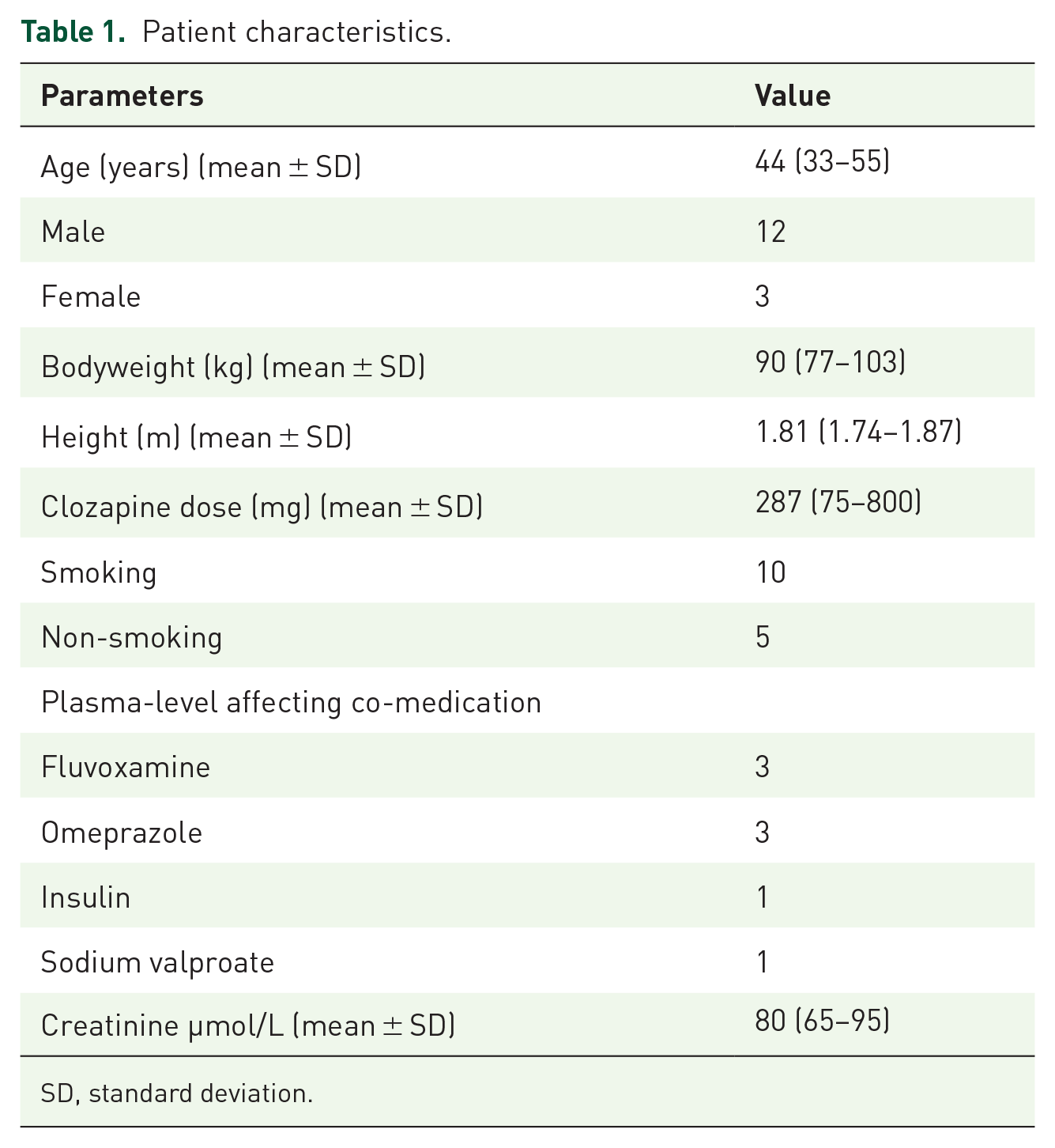
SD, standard deviation.

Results

Study population

In total, 15 patients (12 male/3 female, mean age 44 years) agreed to participate in this study. The baseline characteristics of the included patients are presented in Table 1. For developing the PopPK model, a total of 49 plasma samples and 72 DBS samples were included (Table 2).

Table 2.

Number of collected plasma and DBS samples at each time point.

Sampling time point	plasma samples (N)	DBS samples (N)
0	14	15
2	11	15
4	8	14
6	11	15
8	5	13
Total	49	72

DBS, dried blood spot.

Population PK model

A one-compartment model without lag time gave the best prediction of the described data. The elimination rate (K_el) and distribution volume per kg body weight (V_d) were Bayesian estimated in this model and the absorption rate constant (K_a) was fixed on the original value from the default model since a Bayesian-estimated value did not improve the model, probably due to lack of data in the absorption phase. Adding lag time did not result in a significant decrease in AIC value. Including the distribution of the drug into a peripheral compartment or into fat tissue also did not improve the model. The relatively low number of samples and short time period of 8 h in which all the samples are collected make it difficult to predict inter-compartmental constants. Initial parameters of the default model and developed model are shown in Table 3. The internal validation of the model by bootstrap analysis shows that the model is robust.

Table 3.

Parameters of the default model and final developed PopPk model and bootstrap analysis of this final model.

Parameter	Default model²¹	Clozapine modelFinal (mean ± SD)	Bootstrap analysis (median ± SD)	Shrinkage	CI 95% bootstrap analysis (mean ± SD)
One compartment
K_elm (h^–1)	0.095 ± 0.06	0.0641 ± 0.0365	0.0635 ± 0.0346	0.079	0.0525 ± 0.0214 to 0.0774 ± 0.0504
V_d/F (L/kgLBMc)	9.6 ± 7.6	5.21 ± 3.82	5.20 ± 3.73	0.054	4.12 ± 2.14 to 6.77 ± 5.74
K_a (h^–1)	1.37 ± 0.68	1.37 ± 0.68 (fixed)	1.37 ± 0.68 (fixed)	–	–
T_lag (h)	0	0
AIC	267	-119

AIC, Akaike’s information criterion; K_a, absorption rate constant; K_elm, elimination rate constant; SD, individual standard deviation; T_lag, lag time, variation in the time between intake and start of absorption; V_d/F, volume of distribution/ bioavailability, F was fixed at 1.

By visual inspection of the individual predictive plots (Supplementary Figure 1), the developed PopPK model seems to adequately predict the PK concentration–time curve for individual patients.

In the goodness-of-fit plots (Figure 1), both the population and individual predicted clozapine concentrations are closely distributed along the line of identity. The individual predicted clozapine concentrations are closer distributed around the line of identity compared to the population predicted clozapine concentration, especially for higher concentrations. The weighted residuals of the population predicted clozapine concentrations are relatively close distributed around zero. The time versus weighted residuals plot does not show a major time bias.

Figure 1.

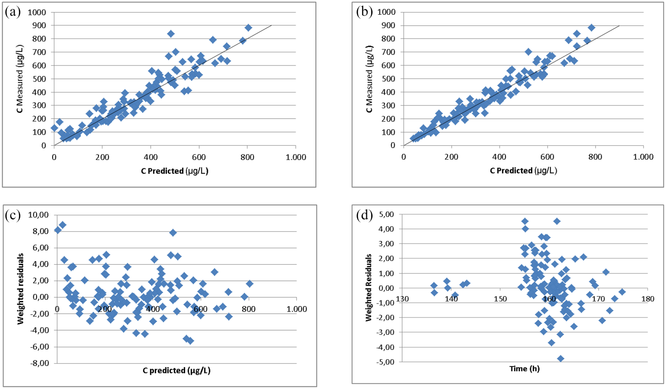
Goodness-of-fit and weighted residual plots of the clozapine concentration: (a) population predicted clozapine levels based on the final model versus the actually measured clozapine levels, (b) individual predicted clozapine levels based on the final model versus the actually measured clozapine levels, (c) weighted residuals of the population predicted clozapine levels versus the predicted clozapine levels, (d) weighted residuals of the population predicted clozapine levels versus time. For modeling and simulation, six till 7 days of clozapine treatment was simulated to have steady state.

LSSs

Based on the PopPK model, LSSs for Bayesian forecasting were evaluated for the time intervals from 0 to 12 h (resembling a two times daily dosing regimen) and 0–24 h (resembling a one times daily dosing regimen). For every time interval, an LSS was developed using one, two, or three sampling points. The optimal combinations based on RMSE value (%), r² value and MPE value (%) all met the requirements set for these values. A sampling model using only trough levels collected 12 h after drug intake was also designed.

For a three–time point sampling scheme, sampling at 2, 6, and 8 h after clozapine intake gave the best prediction of the clozapine AUC_0-12h. The RMSE (%) decreases when the number of sampling points increases. The differences in RMSE (%), MPE (%), and r² value between the best three–time point sampling strategy and a one– or two–time point sampling strategy were small. For clinical practice, sampling time points within a certain time window are preferable. Taken this into account, a two-point sampling strategy with sampling at 2 and 6 h after drug intake is preferable to estimate the AUC_0-12h (RMSE = 9.06%, r² = 0.9954, MPE = −0.20%).

The AUC_0-12h values calculated with all available time points per patients were compared with the AUC_0-12h values calculated with the two-point sampling strategy with sampling at 2 and 6 h. The AUCs_0-12h showed good linearity with each other (r² = 0.9825). The mean difference between the values was 3.9% (Figure 2).

Figure 2.

AUC_(0-12h) based on the full curve compared to AUC_0-12h) calculated with the two-points sampling strategy with sampling at 2 and 6 h.

To estimate the AUC_0-24h with a three–time point sampling strategy, sampling at 4, 10, and 11 h after drug intake gave the best results. However, the differences in RMSE (%), MPE (%), and r² value between a three–time point sampling strategy and a one– or two–time point sampling strategy were small. The RMSE (%) showed again a clear trend for decreasing when the number of included samples increases. Taking clinical practice into account, a two–time point sampling strategy at 4 and 11 h after drug intake is preferable (RMSE = 7.67%, r² = 0.9971, MPE = –0.36%).

The calculated optimal LSSs and selected LSSs for clinical practice (with two sampling points) all gave a better prediction of AUC_0-12h and AUC_024h based on RMSE, r², and MPE values, when compared to a model using only trough level (t = 12). The correlation between AUC_0-12 and the trough level was in general relatively good based on the found r² value (i.e. 0.9710 (Table 4)). The correlation between AUC_0-24 and the trough level was a bit poorer (r² = 0.9374) and did not meet the predefined criterion for a sufficiently predictive model (r² value > 0.95). The above-described LSSs are presented in Table 4.

Table 4.

Predictive value of the limited sampling strategies for clozapine (parameters not meeting the predefined criteria for sufficient predictive strategy are expressed in bolt). .

Dosing interval	First sample	Second sample	Third sample	RMSE (%)	r ²	MPE (%)
0–12	12 (trough level)			23.35	0.9710	5.81
0–12	4			13.04	0.9905	0.56
0–12	2	6		9.06	0.9954	–0.20
0–12	2	6	8	6.87	0.9974	–0.18
0–24	12 (trough level)			34.87	0.9374	1.95
0–24	7			13.58	0.9912	–3.02
0–24	4	11		7.67	0.9971	–0.36
0–24	4	10	11	5.76	0.9984	–0.34

MPE, mean prediction error; RMSE, root mean squared error.

Discussion

In this study, a population PK model was successfully developed that can be used for both clozapine plasma sampling and DBS sampling. Subsequently, LSSs estimating the AUC_0-12h and AUC_0-24h using Bayesian forecasting were developed based on the PopPK model parameterized with all available samples. The AUC is a commonly used marker to estimate drug exposure in time and might be a better predictor for clozapine response or side effects compared to trough level monitoring. The developed model and LSSs meant for Bayesian forecasting can be used to further study this theory. Especially an LSS using DBS sampling makes blood sampling of clozapine much easier and wider accessible because DBS samples are less invasive to collect and highly stable.

For developing the clozapine PopPK model, a total of 49 plasma samples and 72 DBS samples were included. The low number of included patients and collected samples is a disadvantage for the reliability of the PK model and LSS for Bayesian estimating. Also, a lack of samples between 8 and 24 h after clozapine intake (night time during the PK study) might influence the reliability of the model. However, we were able to collect a sufficient number of samples to develop a reliable PopPK modal, and the results from the bootstrap analysis also indicate that the robustness and accuracy of the clozapine PopPK model is sufficient. The goodness-of-fit plots show a close distribution of all data points along the line of identity indicating that the developed PK model adequately predicts clozapine concentrations. Unfortunately, no external validation study was performed to confirm these results.

Another limitation of this study is the change in dosing regimen of several patients. To enable sampling during daytime, patients using a once-daily dosing regimen took half of their evening dose of clozapine the evening before sampling and the other half the next morning. This changed their dosing regimen from a once-daily to a twice-daily dosing regimen. Therefore, only samples were collected when patients were on a twice-daily dosing regimen which makes the applicability to simulations for a once-daily dosing regimen less certain.

In the literature, both one- and two-compartment models for clozapine have been described with a wide range in estimated PK parameters k_el, V_d/F, and K_a.^13,15,21,26 The estimated elimination rate and distribution volume are lower in the developed model compared to the baseline model. The relatively low number of individual patients (N = 15) included in our model may explain this difference because the individual parameters of every patient in this case have a relatively high influence on the ultimately calculated values. Also, in this study, only patients with a Western European descent were included, which might have an influence on the generalizability of the model and LSS.

For the PopPK model, we were unable to collect plasma samples at all predefined data points for every patient. Repeated venous blood sampling was experienced as too uncomfortable by some patients. None of the patients preferred venous blood collection by a peripheral indwelling cannula. From the DBS samples, 72 of the 75 planned samples were collected. This confirms the presumption that DBS sampling is experienced as less burdensome for drug concentration measurement compared to the regular venous blood sampling method.¹⁸

Another limitation of our study is that we did not include covariates such as smoking, infection/inflammation, and drug–drug interactions in our model. Some patients were smoking and some had interacting drugs. These covariates will have contributed to the residual variance of the model and the LSS thus takes this into account. The high predictive performance of the LSS in combination with the population PK model and Bayesian forecasting demonstrates that the approach leads to reliable estimations of the AUC.

For the LSSs for Bayesian forecasting, a three-sampling point’s strategy appears to give the best estimation of the clozapine AUC_0-12 and AUC_0-24. To keep the method patient friendly, the number of samples for the LSS was limited to a maximum of three. Samples taken more than 12 h after drug intake appeared to have a minor influence on AUC. The best two–time point sampling strategies were only slightly less predictive for the AUCs compared to the best three–time point sampling strategies. Therefore, we prefer the use of these two–time point strategies for daily and research practice.

In both cases, trough levels gave a poorer prediction of the AUC_0-12 and AUC_0-24 when compared to the optimally scheduled samples and did not meet our criteria as sufficient predictive (r² value > 0.95, an RMSE value < 15%, and MPE value < 5%). The correlation between trough level and AUC_0-12 was in general better than with AUC_{0-24 h} (Table 4). This implies that the trough level cannot be used as surrogate for AUC_0-24. Since AUC is commonly seen as a good marker to estimate drug exposure, our limited sampling model might be a better predictor for effects of clozapine compared to trough level monitoring.

Previously, Perera et al.¹⁵ made a literature based LSS for several antipsychotic drugs, including clozapine. Their optimal sampling time points include a sampling point in the absorption phase (T = 1.1 h), around T_max (T = 4.6 h) and in the elimination phase (T = 12) of the PK curve. The results are in line with the optimal sampling points found in this study; however, time points 1.1 and 4.6 h are less practical than our suggested time points. The correlation between clozapine AUC and the trough level was found sufficient by Perera et al. (r² = 0.93), a result that was comparable to results in our study. Nevertheless, trough level measurement did not meet our criterion for a sufficient predictive LSS.

For daily practice, trough level monitoring might be sufficient, given the relatively wide therapeutic range of clozapine.^12
–14 On the contrary, the wide therapeutic range may be the result of the poor predictive performance of the trough level for the AUC and thus exposure. Whether AUC is a better predictor for efficacy and toxicity remains to be elucidated. To investigate this, the two–time point sampling strategies developed in this study can be used.

Conclusion

In conclusion, a population PK model and two LSSs meant for Bayesian forecasting were successfully developed for both twice (AUC_0-12h) and once daily (AUC_0-24h) dosing regimens of clozapine. A two–time point LSS, with sampling points at 2 and 6 hours for AUC_0-12h and at 4 and 11 hours for AUC_0-24h, can best be used for predicting the clozapine exposure in time expressed as AUC. These strategies give a better prediction of the clozapine exposure in time, expressed as AUC, compared to though level monitoring and might therefore be a better predictor for clinical response. DBS sampling for clozapine is better accepted by patients for blood sampling of clozapine compared to the regular venous blood sampling method. A two–time point LSS meant for Bayesian forecasting using DBS sampling, therefore makes studying clozapine exposure in time much easier and wider applicable.

Supplemental Material

sj-pptx-1-tpp-10.1177_20451253211065857 – Supplemental material for Population pharmacokinetic model and limited sampling strategy for clozapine using plasma and dried blood spot samples

Supplemental material, sj-pptx-1-tpp-10.1177_20451253211065857 for Population pharmacokinetic model and limited sampling strategy for clozapine using plasma and dried blood spot samples by Lisanne M. Geers, Dan Cohen, Laura M. Wehkamp, Hans J. van Wattum, Jos G.W. Kosterink, Anton J.M. Loonen and Daan J. Touw in Therapeutic Advances in Psychopharmacology

Footnotes

Author contributions

Lisanne M. Geers: Formal analysis; Investigation; Writing – original draft

Dan Cohen: Conceptualization; Supervision; Writing – review & editing

Laura M. Wehkamp: Investigation; Writing – review & editing

Hans J. van Wattum: Investigation; Writing – review & editing

Jos G.W. Kosterink: Conceptualization; Writing – review & editing

Anton J.M. Loonen: Conceptualization; Supervision; Writing – review & editing

Daan J. Touw: Conceptualization; Supervision; Writing – review & editing

Conflict of interest statement

The authors declared no potential conflicts of interest with respect to the research, authorship, and/or publication of this article.

Funding

The authors received no financial support for the research, authorship, and/or publication of this article.

ORCID iD

Lisanne M. Geers

Availability of data

The data that support the findings of this study are available from the corresponding author upon reasonable request.

Supplemental material

Supplemental material for this article is available online.

References

Azorin

Spiegel

Remington

, et al A double-blind comparative study of clozapine and risperidone in the management of severe chronic schizophrenia. Am J Psychiatry 2001; 158: 1305–1313.

Conley

Tamminga

Kelly

, et al Treatment-resistant schizophrenic patients respond to clozapine after olanzapine non-response. Biol Psychiatry 1999; 46: 73–77.

Takeuchi

Powell

Geisler

, et al Clozapine administration in clinical practice: once-daily versus divided dosing. Acta Psychiatr Scand 2016; 134: 234–240.

Khan

Preskorn

. Examining concentration-dependent toxicity of clozapine: role of therapeutic drug monitoring. J Psychiatr Pract 2005; 11: 289–301.

Hiemke

Baumann

Bergemann

, et al AGNP consensus guidelines for therapeutic drug monitoring in psychiatry: update 2011. Pharmacopsychiatry 2011; 44: 195–235.

Spina

Avenoso

Facciola

, et al Relationship between plasma concentrations of clozapine and norclozapine and therapeutic response in patients with schizophrenia resistant to conventional neuroleptics. Psychopharmacology 2000; 148: 83–89.

Hiemke

Bergemann

Clement

, et al Consensus guidelines for therapeutic drug monitoring in neuropsychopharmacology: update 2017. Pharmacopsychiatry 2018; 51: 9–62.

Pfuhlmann

Hiemke

Unterecker

, et al Toxic clozapine serum levels during inflammatory reactions. J Clin Psychopharmacol 2009; 29: 392–394.

Rostami-Hodjegan

Amin

Spencer

, et al Influence of dose, cigarette smoking, age, sex, and metabolic activity on plasma clozapine concentrations: a predictive model and nomograms to aid clozapine dose adjustment and to assess compliance in individual patients. J Clin Psychopharmacol 2004; 24: 70–78.

10.

Potkin

Bera

Gulasekaram

, et al Plasma clozapine concentrations predict clinical response in treatment-resistant schizophrenia. J Clin Psychiatry 1994; 55(Suppl. B): 133–136.

11.

Buur-Rasmussen

Brosen

. Cytochrome P450 and therapeutic drug monitoring with respect to clozapine. Eur Neuropsychopharmacol 1999; 9: 453–459.

12.

Schulte

. What is an adequate trial with clozapine? Therapeutic drug monitoring and time to response in treatment-refractory schizophrenia. Clin Pharmacokinet 2003; 42: 607–618.

13.

Liu

Chang

Wei

, et al Monitoring of plasma clozapine levels and its metabolites in refractory schizophrenic patients. Ther Drug Monit 1996; 18: 200–207.

14.

Netherlands Clozapine Collaboration Group, 2013, http://www.clozapinepluswerkgroep.nl/wp-content/uploads/2013/07/Guideline-for-the-use-of-Clozapine-2013.pdf

15.

Perera

Bies

, et al Optimal sampling of antipsychotic medicines: a pharmacometric approach for clinical practice. Br J Clin Pharmacol 2014; 78: 800–814.

16.

Shang

Wang

, et al Population pharmacokinetic/pharmacodynamic model of clozapine for characterizing the relationship between accumulated exposure and PANSS scores in patients with schizophrenia. Ther Drug Monit 2014; 36: 378–386.

17.

Green

Duffull

. Prospective evaluation of a D-optimal designed population pharmacokinetic study. J Pharmacokinet Pharmacodyn 2003; 30: 145–161.

18.

van der Elst

Span

van Hateren

, et al Dried blood spot analysis suitable for therapeutic drug monitoring of voriconazole, fluconazole, and posaconazole. Antimicrob Agents Chemother 2013; 57: 4999–5004.

19.

Geers

Cohen

Wehkamp

, et al Dried blood spot analysis for therapeutic drug monitoring of clozapine. J Clin Psychiatry 2017; 78: e1211–e1218.

20.

Edelbroek

van der Heijden

Stolk

. Dried blood spot methods in therapeutic drug monitoring: methods, assays, and pitfalls. Ther Drug Monit 2009; 31: 327–336.

21.

Jerling

Merle

Mentre

, et al Population pharmacokinetics of clozapine evaluated with the nonparametric maximum likelihood method. Br J Clin Pharmacol 1997; 44: 447–453.

22.

College ter beoordeling van geneesmiddelen. SMPC Leponex 100mg, https://www.geneesmiddeleninformatiebank.nl/ords/f?p=111:3::SEARCH:NO::P0_DOMAIN, P0_LANG,P3_RVG1:H,NL,10460 (2014, accessed 25 November 2020).

23.

Proost

Eleveld

. Performance of an iterative two-stage Bayesian technique for population pharmacokinetic analysis of rich data sets. Pharm Res 2006; 23: 2748–2759.

24.

van den Elsen

SHJ

Sturkenboom

MGG

Van’t Boveneind-Vrubleuskaya

, et al Population pharmacokinetic model and limited sampling strategies for personalized dosing of levofloxacin in tuberculosis patients. Antimicrob Agents Chemother 2018; 62: e01092-18.

25.

Westra

Proost

Franssen

, et al Vancomycin pharmacokinetic model development in patients on intermittent online hemodiafiltration. PLoS ONE 2019; 14: e0216801.

26.

Guitton

Kinowski

Gomeni

, et al A kinetic model for simultaneous fit of clozapine and norclozapine concentrations in chronic schizophrenic patients during long-term treatment. Clin Drug Investig 1998; 16: 35–43.

Supplementary Material

Please find the following supplemental material available below.

For Open Access articles published under a Creative Commons License, all supplemental material carries the same license as the article it is associated with.

For non-Open Access articles published, all supplemental material carries a non-exclusive license, and permission requests for re-use of supplemental material or any part of supplemental material shall be sent directly to the copyright owner as specified in the copyright notice associated with the article.

0.00 MB

0.97 MB