
Abstract
Background:
Severe cutaneous adverse reactions (SCARs) are prominent in pharmacovigilance (PhV). They have some commonalities such as nonimmediate nature and T-cell mediation and rare overlap syndromes have been documented, most commonly involving acute generalized exanthematous pustulosis (AGEP) and drug rash with eosinophilia and systemic symptoms (DRESS), and DRESS and toxic epidermal necrolysis (TEN). However, they display diverse clinical phenotypes and variations in specific T-cell immune response profiles, plus some specific genotype–phenotype associations. A question is whether causation of a given SCAR by a given drug supports causality of the same drug for other SCARs. If so, we might expect significant intercorrelations between SCARs with respect to overall drug-reporting patterns. SCARs with significant intercorrelations may reflect a unified underlying concept.
Methods:
We used exploratory factor analysis (EFA) on data from the United States Food and Drug Administration Adverse Event Reporting System (FAERS) to assess reporting intercorrelations between six SCARs [AGEP, DRESS, erythema multiforme (EM), Stevens–Johnson syndrome (SJS), TEN, exfoliative dermatitis (ExfolDerm)]. We screened the data using visual inspection of scatterplot matrices for problematic data patterns. We assessed factorability via Bartlett’s test of sphericity, Kaiser-Myer-Olkin (KMO) statistic, initial estimates of communality and the anti-image correlation matrix. We extracted factors via principle axis factoring (PAF). The number of factors was determined by scree plot/Kaiser’s rule. We also examined solutions with an additional factor. We applied various oblique rotations. We assessed the strength of the solution by percentage of variance explained, minimum number of factors loading per major factor, the magnitude of the communalities, loadings and crossloadings, and reproduced- and residual correlations.
Results:
The data were generally adequate for factor analysis but the amount of variance explained, shared variance, and communalities were low, suggesting caution in general against extrapolating causality between SCARs. SJS and TEN displayed most shared variance. AGEP and DRESS, the other SCAR pair most often observed in overlap syndromes, demonstrated modest shared variance, along with maculopapular rash (MPR). DRESS and TEN, another of the more commonly diagnosed pairs in overlap syndromes, did not. EM was uncorrelated with SJS and TEN.
Conclusions:
The notion that causality of a drug for one SCAR bolsters support for causality of the same drug with other SCARs was generally not supported.
Introduction
Severe cutaneous adverse reactions (SCARs) are a prominent issue in drug safety given their potential seriousness and associations with numerous medicines [Mockenhaupt et al. 2008; Mockenhaupt, 2009]. The definition of SCARS is variable but a typical set includes toxic epidermal necrolysis (TEN), Stevens–Johnson syndrome (SJS), erythema multiforme (EM) major, drug rash with eosinophilia and systemic symptoms (DRESS), acute generalized exanthematous pustulosis (AGEP) and linear IgA bullous dermatosis (LiIgAD) [Mockenhaupt et al. 2008; Mockenhaupt, 2009].
These nonimmediate reactions demonstrate commonalities and differences, and overlap syndromes exist [Bouvresse et al. 2012; Bouvresse et al. 2012]. For example, all have a common base of CD4+ and CD8+ lymphocyte mediation but the relative distribution of such T-cell-specific mediator pathways and clinical phenotypes vary [Rozieres et al. 2009]. Furthermore, there are very specific genotype–phenotype associations for some drugs, for example, carbamazepine [Hsiao et al. 2014].
From the perspective of pharmacovigilance (PhV) risk or causality assessment, a natural question is whether accepted causality between a drug and one type of T-cell-mediated SCAR bolsters the case for causality for the same drug and other T-cell-mediated SCARs? In fact, the motivation for the current investigation was a real-world PhV committee deliberation that one of the authors (MH) participated in, in which this notion was submitted for consideration.
For some, such as EM, SJS and TEN, that represent a pathophysiological continuum [Roujeau, 2013], the answer would probably be ‘yes’. But what about others, for which the link is not as clear cut? Does occurrence of AGEP due to a drug bolster the argument for causality in reports of SJS with the same drug? Do SCARS reported in rare overlap syndromes such as DRESS and AGEP, and DRESS and SJS-TEN [Bouvresse et al. 2012] display significant intercorrelations in terms of reported suspect drugs? Significant intercorrelations between SCARS and overall drug-reporting patterns would support this notion.
There is considerable published literature on the quantitative associations between individual drugs and SCARs. RegiScar is a prominent multinational initiative studying bivariate (i.e. drug-individual SCAR) relationships [Mockenhaupt et al. 2008]. These bivariate perspectives are important but to the best of our knowledge, there are no systematic studies of the higher-level networks of interrelationships (i.e. patterns) between SCARs and reported suspect drugs.
The objective of this investigation is to shed light on the above causality assessment question by seeking intercorrelations between various SCARs and suspect drugs using exploratory factor analysis (EFA). Expressed a little differently, are SCARs resolvable into distinct event clusters with highly covariant drug reporting patterns representing underlying concepts?
Methodology
We analyzed a Freedom of Information (FOI) abstract of the United States Food and Drug Administration Adverse Event Reporting System (FAERS) database (DB) representing reports entered from 1968 through the first quarter of 2014 [US Food and Drug Administration, 2016]. The FAERS DB contains spontaneous reports of adverse events (AEs) and medication errors submitted to the US Food and Drug Administration (FDA). The DB is designed to support the FDA’s postmarketing safety surveillance program for drug and therapeutic biologic products. AEs and medication errors are coded using the Medical Dictionary for Regulatory Activities (MedDRA) terminology. The default unit of observation in general PhV is the MedDRA Preferred Term (PT) which is intended to represent a distinct medical concept [Kübler et al. 2005].
For the purposes of this analysis, we considered SCARs to include PTs TEN, SJS, EM, DRESS, AGEP, LiIgAD, and generalized exfoliative dermatitis (ExFolDerm). In addition we included two skin events as quasi-negative controls: psoriasis and maculopapular rash (MPR). Because diagnostic confusion may exist between TEN and generalized bullous fixed drug eruption [Baird and De Villez, 1988], we planned to include it as an event, but this entity is not precisely represented in MedDRA (defaulting to ‘drug eruption’).
We extracted data for all drugs that were listed as a suspect drug in at least one spontaneous report of any of the selected SCARs. For each drug, we calculated an observed-to-expected (O/E) spontaneous reporting frequency, that is, disproportionality analysis (DA). DA is widely used to ascertain statistical reporting associations in spontaneous reporting systems (SRS). [Hauben and Bate, 2009]. The O/E calculated by DA represents how much more frequently an event is being reported with a drug compared with what would be expected if drug and event were independently recorded in the DB. An O/E above a selected threshold may be a signal of an underlying causal association depending on the clinical context [Hauben and Aronson, 2009; Hauben and Bate, 2009]. DA has previously been used to investigate spontaneous reporting of dermatological adverse drug reactions [Hauben et al. 2008]. The O/E metric used in this form of DA is the empirical Bayesian geometric mean (EBGM), calculated by an empirical Bayesian implementation of DA known as the multi-item Gamma-Poisson shrinker (MGPS) [Hauben and Bate, 2009].
EFA is a multivariate technique with an attractive and accessible geometric interpretation [Rummel, 1967; Spicer, 2005; Yong and Pearce, 2013]. In effect, we construct a high-dimensional geometric space in which each axis represents a drug and the scale of each axis is in units of standardized O/E spontaneous reporting frequency. Highly intercorrelated SCARs in close geometric proximity in this space may be considered to show substantial shared variability and reflect a unified underlying concept. An example of an expected underlying factor or construct might be EM-SJS-TEN.
Each factor represents an additive combination of one or more of the original variables and ideally captures the essence of the data in a lower dimensional representation. They are obtained by progressively decomposing the original data covariance or correlation matrix into a series of matrices representing shared and residual covariance. In other words, it aims to condense the data into a reduced number of interpretable variables capturing most of the inter-relationships in the data (i.e. closely reproducing the correlation matrix of the original data). A self-contained EFA tutorial and glossary are provided in Appendices A and B to help readers unfamiliar with the technique read the manuscript.
A distinction has been made between absolute versus heuristic uses of EFA [Darlington, 1997]. The purpose of EFA in the context of our analysis is heuristic, providing a useful way to organize, summarize, condense and visualize data to better understand its structure, even if this summary is not true in an absolute sense. Our use of EFA varies from the typical application in that knowing whether or which SCARs are interrelated, and which are not, are both pertinent to our research question on causality assessment. In other words, while positive findings are usually considered most interesting and glamorous, negative findings are informative as well.
As a quality check, and to guard against the possibility of the results being significantly dependent on software implementation, we ran three default analyses. The first was performed by one author (MH), using SPSS 22. Another author (EH), reproduced the analysis with the same software. Finally, the third author (AH), ran the analysis in R.
The data was screened for factorability using several well described criteria including sample size or variable ratio, Kaiser–Myer–Olkin (KMO) measure of sample adequacy, Bartlett’s test of sphericity, anti-image correlations, [Costello and Osborne, 2005; Spicer, 2005; Matsunaga, 2010; Beavers et al. 2013]. Since we were interested in determining which variables were related versus unique, we departed from the common practice of using the factorability screen for item reduction and used it to specifically address overall factorability.
We extracted factors using principle axis factoring (PAF) with different rotation methods. To maximally accommodate the possibility of unexpected correlations among distinct SCARS, we chose oblique (nonorthogonal) rotation since this can also return orthogonal solutions, if those are most appropriate and emerge naturally from the data [Spicer, 2005]. Specifically, we performed separate analyses using obliquemin versus varimax versus Promax oblique rotation. The number of factors to retain was based on the Kaiser rule and visual inspection of a scree plot. Because the latter methods may be associated with a tendency to underextract factors [Fabrigar et al. 1999], we also performed an analysis with an additional factor. The quality or stability of the factor solution was assessed by several indicators, including the minimum number of variables loading per major factor, magnitudes of the loadings and crossloadings, and residual and reproduced correlations. [Costello and Osborne, 2005; Spicer, 2005; Matsunaga, 2010; Beavers et al. 2013].
Unlike the other major Bayesian implementation of DA, the Bayesian Confidence Propagation Neural Network (BCPNN), MGPS does not return results for drug-event combinations (DECs) without reports. For these DECs we considered the O/E to be zero in default analysis because this was the most concrete physical interpretation. Another interpretation, implemented in BCPNN, is that in the absence of prior information, a default O/E ratio of one is returned. To assess the robustness of findings against these interpretations we reran the analysis using a series of O/E ratios between 0 and 1 including random draws from a uniform distribution with a range of 0,1 U[(0,1)].
The question of transforming non-normal, skewed, asymmetric variables towards normality or greater symmetry is important for EFA, which is based on interitem correlations, since the usual correlation measure, Pearson’s r, is influenced by skewness and outliers. We decided to use untransformed data for our primary analysis because: (1) our data represented a census of all cases meeting criteria and not a sample from which we extrapolate to the population via inferential testing and confidence statements; (2) the size of our census population; (3) priority given to preserving scientific meaningfulness of the variables used; (4) scientific assessment that the most extreme outliers were valid representations of the natural phenomenon under study; (5) our use of exploratory, rather than confirmatory factor analysis. Nonetheless, we examined the scatterplot matrix displaying the bivariate correlations between pairs of SCARs to screen for severe skew or U-shaped or inverted U-shaped patterns that could obscure the relationship when using a linear measure of dependence like Pearson’s r [Goldberg and Velicer, 2006].
Results
The results returned by SPSS were clearly consistent with, if not numerically identical to, the results returned by R. Herein, we present the results from SPSS.
There were 84,470 spontaneous reports recording 2559 unique suspect drugs from diverse pharmacological or therapeutic classes involving one or more of the nine selected SCARS and quasi-negative control events. By PT, the corresponding report frequencies were: MPR (1714), SJS (1591), TEN (1355), EM (1260), Psoriasis (870), DRESS (778), AGEP (580), LIgAD (143), and ExFolDerm (72). The sample size well exceeds minimal sample size recommendations [Costello and Osborne, 2005; Spicer, 2005; Matsunaga, 2010; Beavers et al. 2013]. The ratio of objects (i.e. drugs)-to-items (284/1) is also well in excess of the minimum 10/1 ratio typically recommended for EFA, which is a large sample method [Costello and Osborne, 2005; Spicer, 2005; Matsunaga, 2010; Beavers et al. 2013]. No U-shaped or inverted U-shaped patterns were appreciated in the scatterplot matrix of the pairwise correlations between SCARs. However, the scatterplots demonstrated ‘dust bunny’ patterns, indicative of substantially, positively skewed distributions (scatterplot matrix not shown).
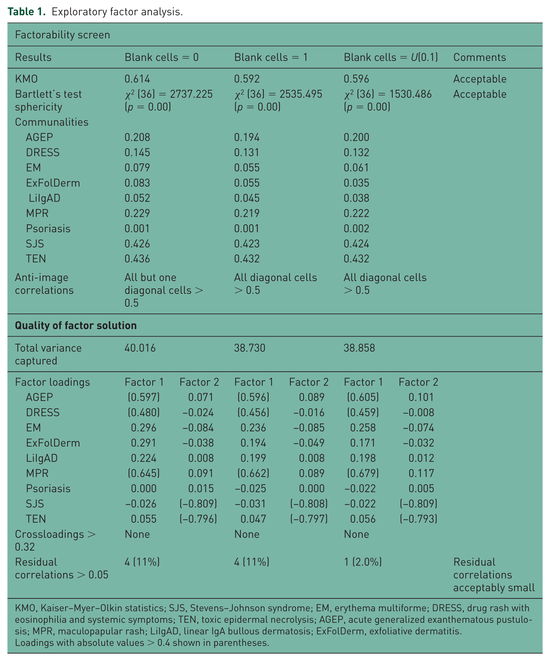
The factorability of the data was acceptable based on sample size, KMO measure of sample adequacy, Bartlett’s test of sphericity, initially estimated communalities and anti-image correlations (Table 1). The KMO measure of sampling adequacy (KMO = 0.592–0.614) supports adequate, though not so-called ‘meritorious’ (KMO > 0.8) or ‘marvelous’ (KMO > 0.9) [Spicer, 2005] common variance for factor analysis. Bartlett’s test of sphericity was significant (χ2 (36) = 1530.486–2737.225; p = 0.00) suggesting the correlation matrix was significantly different from the identity matrix and therefore factorable. With one exception, the diagonals of the anti-image correlation matrix were all >0.5. The overall data screen points to an acceptable, if suboptimally factorable, correlation matrix.
Exploratory factor analysis.
KMO, Kaiser–Myer–Olkin statistics; SJS, Stevens–Johnson syndrome; EM, erythema multiforme; DRESS, drug rash with eosinophilia and systemic symptoms; TEN, toxic epidermal necrolysis; AGEP, acute generalized exanthematous pustulosis; MPR, maculopapular rash; LiIgAD, linear IgA bullous dermatosis; ExFolDerm, exfoliative dermatitis.
Loadings with absolute values > 0.4 shown in parentheses.
Kaiser’s rule and visual inspection of scree plot (Figure 1) identified two factors for extraction that explained only 38.730–40.858% of the variance corresponding to two empirically distinct clusters of SCARs. The communalities were quite variable and often low, already an indication that SCARs do not exhibit substantial shared reporting behavior. SJS and TEN showed clear geometric proximity and the highest communalities, loading heavily onto factor 2 without significant crossloading, consistent with a single unifying concept, distinct from other SCARs and skin reactions studied. Factor 1 primarily represents DRESS, AGEP and MPR, which have lower loadings than SJS-TEN on factor 2, but again, without significant crossloading. Different forms of oblique rotation returned consistent solutions. Figures 2 and 3 are factor plots showing the distribution and correlations of the various SCARs in two dimensions (with obliquemin and promax rotation). Interestingly, EM did not cluster with SJS and TEN.
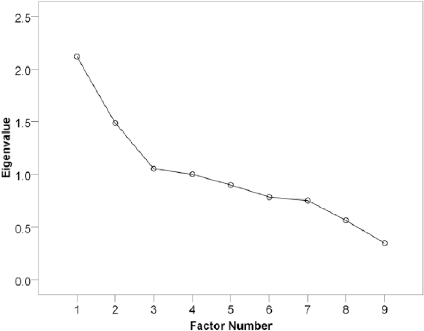
Scree plot.
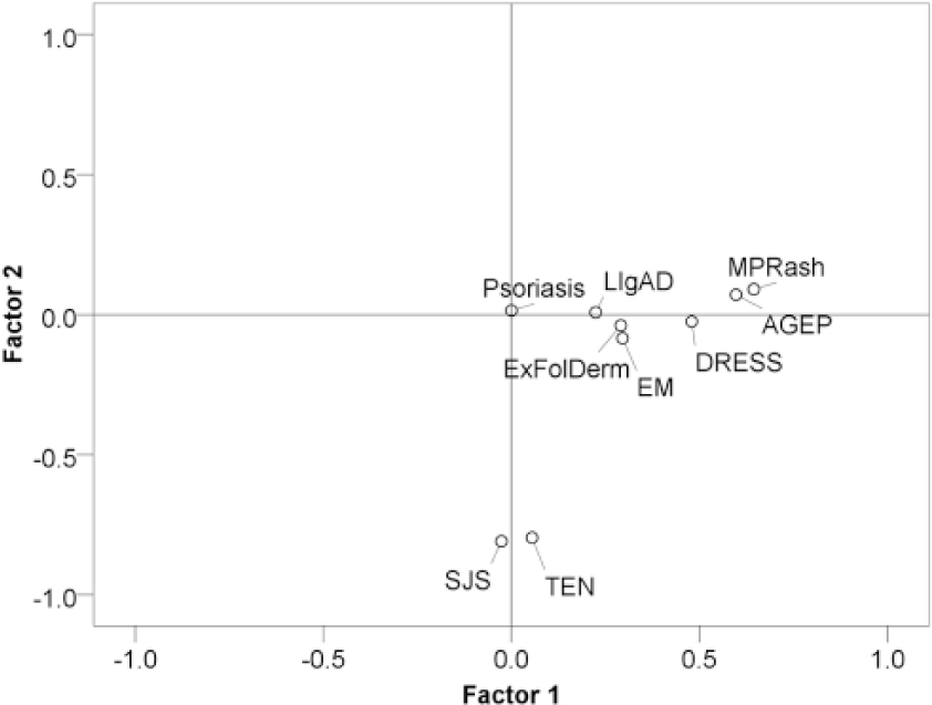
Factor plot in rotated factor space – obliquemin.
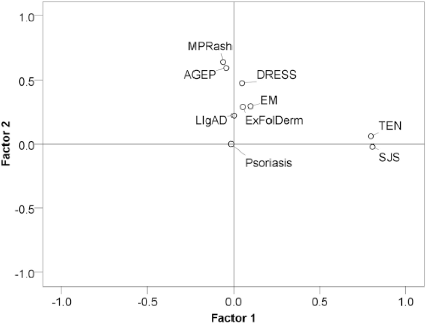
Factor plot in rotated factor space – promax.
Solutions extracting additional factors were not retained because of one or more of the following: convergence failure, absence of strong loadings on the additional factor(s), with or without significant crossloadings; in other words, a less clear factor resolution.
Discussion
Our analysis suggests that SCARS are generally dissimilar with respect to patterns of recorded suspect drugs. In other words, only a small percentage of drug reporting patterns of most SCARs are predictable from results with other SCARs. However, we did discern some higher-order intercorrelations of interest, and this is the motivation for performing EFA. Since correlation is not transitive, that is, A correlating with B, and B correlating with C, does not necessarily indicate that A correlates with C (except when the first two correlations are sufficiently large), examining a only a subset of pair-wise correlations may be misleading [Langford, 2001]. One cannot even prospectively ensure that higher-order covariance patterns are revealed by inspecting a full matrix of all pairwise correlations.
SJS and TEN demonstrated the most shared variance and largest communalities. These two variables loading onto the major factor are less than the usual recommendation of three heavily loading variables per factor without significant crossloading. However, if highly correlated, even two factors loading onto a major axis are acceptable [Yong and Pearce, 2013].
AGEP and DRESS, along with MPR, showed modest resemblance in drug-reporting patterns, but again, based on a modest amount of the shared variance and low communalities. Nonetheless, this is interesting, relative to the overlap syndromes studied by RegiSCAR [Bouvresse et al. 2012]. Structured definitional criteria were applied to 383 registry cases with a diagnosis of at least one of the following SCARS: AGEP, DRESS, SJS-TEN and ‘drug rash’. There were three cases adjudicated as true overlap syndromes: one was AGEP and DRESS, and two cases were diagnosed as SJS-TEN-DRESS overlap.
Therefore, based on spontaneous reporting patterns, our results support a general circumspection in extrapolating causality for a given drug across SCARs. In particular, our analysis does not support extrapolating causal reasoning from less serious SCARs to SJS/TEN, which demonstrated the highest correlations. The remaining SCARs did not demonstrate notably similar drug-reporting patterns. The lesser intercorrelation of AGEP, DRESS and MPR must be interpreted cautiously, given the modest levels of communality.
Our findings have plausible clinical correlations. The two SCARs that clustered tightly together (SJS and TEN) are considered related entities on a severity spectrum (e.g. body surface area involved). EM is often included in this clinical continuum, but it was distant from SJS and TEN in EFA, likely representing a shift in reporting patterns towards antimicrobial drugs with potential for confounding by infection indications. Also, the results may be influenced by diagnostic accuracy at the bedside. SJS and TEN have dramatic presentations that may be less likely to be misdiagnosed than less severe, dramatic, or phenotypically less specific SCARs. Misdiagnosis of some SCARs (e.g. AGEP versus psoriasis) could blur reporting relationships. Somewhat mitigating this concern is that even less serious SCARs, such as LiIgABD can still have distinctive clinical phenotypes. The clustering of MPR with AGEP and DRESS may reflect, at least in part, that DRESS may include a maculopapular morphology.
There are important limitations related to our data and method. The numerous weaknesses of SRS data make such quantitative analysis nonprobative but rather, one element to be considered within a holistic framework, that is, as a hypothesis-generating or -refining exercise, rather than hypothesis testing. As previously discussed, we view our analysis as a hypothesis-refining exercise to address a question related to real-world causality assessment. The voluntary nature of spontaneous AE reports leads to under-reporting in general; however, reporting for specific drugs can be stimulated by external factors such as media attention and litigation that can selectively skew spontaneous reporting. Furthermore, spontaneous reports must pass through various nonrandom filters, including AE coding practices and report inclusion or exclusion criteria before being memorialized in a health authority SRS DB, potentially violating a key assumption of DA if these filters are drug selective [CIOMS, 2010]. AE reporting patterns may also be a function of the time point of observation in the drug’s life cycle, for example, the Weber effect [Hartnell et al. 2004], which can complicate comparisons, especially frequency-based comparisons, though DA should be relatively robust to secular trends in marginal drug or event reporting. Other artifacts may complicate interpretation of quantitative analysis of SRS data such as masking, [Maignen et al. 2014a, 2014b] that could be pertinent to the current analysis. Also DA metrics are influenced by the overall safety profiles of drugs, for example, other events strongly associated with a drug may dampen the statistical association of the drug with the event of interest (in effect, a drug masking itself), so-called event competition bias [Salvo et al. 2013]. Finally, spontaneous reports are often unconfirmed.
We used one variant of DA (MGPS). MGPS attempts to control false-positive findings using one form of empirical Bayesian shrinkage. While an elegant option for mitigating the burden of false-positive findings, it ‘might obfuscate a real signal by reducing it to a nonconspicuous level.’ [Suling and Pigeot, 2012]. Hence, it is possible that the O/Es returned for some DECs might be inappropriately low. Other DAs may have returned somewhat different findings.
Distributional properties of data are often cited as additional limitations for EFA. Multivariate analysis methods may entail assumptions of multivariate normality, linearity and homoscedasticity, violations of which have more or less impact depending on the assumption, the method and the sample size. For EFA, which is essentially a form of correlational analysis, different distribution shapes and skewness impact observed correlations, as well as the maximum observable correlation, that is, the ‘moving ceiling’ effect, [Halperin, 1986; Dunlap et al. 1995; Goldberg and Velicer, 2006]. Since the interpretation of the significance of an observed correlation is roughly contextualized via its maximum possible value, differently shaped, with or without skew, distributions potentially complicate its interpretation.
However, meeting assumptions is not as much a concern with EFA which does not typically entail inferential statements about statistical significance or confidence. In addition, there are statistical arguments supportive of correlational analysis for differently shaped, even asymmetrical, non-normal distributions [Schatschneider and Lonigan, 2010]. Furthermore, the method of factor extraction we used, PAF, does not entail distributional assumptions, unlike factor extraction based on maximum likelihood. Finally, we analyzed all reports, not a sample from which we make inferences. We therefore tailored the methodology to the context using the physically meaningful untransformed data. Nonetheless, examining the results after normalizing or symmetrizing transformations, as well as from robust EFA methods, would be a logical extension of the present analysis.
Another assumption of EFA is independence of observations. This may be violated with DA of SRS data on two counts. First, in a DB of fixed size, an increase in some O/E ratios must be accompanied by a decrease in others. In addition, multiple drugs and events may be recorded per report, and the MedDRA dictionary is hypergranular, so these events are often clinically, and possibly conceptually related and therefore not truly independent observations.
Our sensitivity analysis is potentially a significant limitation. It was based on assuming that an absence of reports of a given drug–SCAR combination indicates independence or an inverse-reporting relationship, when in fact there can be many reasons that a given DEC is not reported. While we had plausible justifications for these interpretations, our use of U(0.1) may have been constraining. Random draws from a uniform or other distribution with a wider range may have clearly provided a more robust sensitivity analysis.
The use of scree plots/Kaiser’s rule for determining the number of factors to extract may result in underextracting factors, and methodologists appear to express more concerns with underfactoring than overfactoring. Underfactoring is a concern because variables that would have loaded onto omitted factors spuriously load onto the extracted factors, which can also affect the loadings of variables that appropriately load onto the included factors [Fabrigar et al. 1999]. To mitigate this concern, we supplemented our default two-factor solution with a three-factor solution that we rejected due to a lack of a clear-factor resolution.
EFA is somewhat controversial in that it has been described as more art than statistical science without absolute guidelines, and therefore, not as objective as other multivariate methods. Some even recommend against its use in general. An EFA should not be viewed as a single definitive solution but one solution out of many that could have been obtained. However, our findings were more or less consistent across analytical choices and solutions. Our view is in line with Manley: ‘If it is thought of as a purely descriptive tool, with limitations that are understood, then it must take its place as one of the important multivariate methods’ [Manly, 2004].
In summary, we did not find substantial intercorrelations among SCARs in terms of drug-reporting patterns. SJS and TEN displayed the most shared variance, followed by AGEP, DRESS, and MPR. Our results do not support cross-SCAR extrapolation of causality from less serious to the most serious SCARS, SJS and TEN, which seem to be distinctive. Given the limitations of both the data and method, these results are inconclusive as stand-alone findings, but may be one element to consider in the context of multiple methods and data streams.
Finally, we hope that our paper increases awareness and understanding of elegant multivariate methods, and their more modern extensions, among drug-safety professionals. They can potentially enhance situational awareness of adverse drug-event reporting patterns. For example we are currently investigating the application of multivariate methods, including EFA, to understand spontaneous reporting patterns involving drug abuse liability [Hauben, 2015], eosinophilc syndromes and interstitial lung disease, to name a few.
Footnotes
Appendix A: Introduction to exploratory factor analysis concepts
We illustrate the basic concepts of EFA with an unrealistically oversimplified and fictitious data set. Table A1 displays data underlying a three-dimensional drug space. Each cell entry is a fictitious O/E reporting measure.
Each drug and event may be considered a vector. The components of the drug vector consist of the ‘event-specific’ O/E ratios for each drug. For example, the drug A vector can be depicted as [2,6,6,5,1]. Thus, each drug vector is five-dimensional and can be plotted in a five-dimensional space, with each number in a vector representing the projection of that vector onto one of the axes. Traditionally, this is referred to as subject space. The components of the event vectors consist of ‘drug-specific’ O/E ratios and are therefore three-dimensional (because there are three drugs in this fictitious data set). For example, the DRESS vector is [2,1,1]. The event vectors can therefore be plotted in a three-dimensional variable space, which we do in Figure A1. One can see that SCARs that tend to have high O/Es with the same drugs and low O/E ratios with the same drugs will result in vectors that are tightly clustered in drug space.
From this fictitious and oversimplified DB, we might understandably wonder whether these five SCARs actually represent 2 distinct underlying disease entities represented by the two clusters (DRESS-psoriasis and EM-SJS-TEN). If so, then we have achieved a simplified and more understandable interpretation of the data. However, even in this simplified data set, we cannot reliably quantify how distinct they are by just eyeballing the data matrix. In real life, there will be many more variables that in total, may not be so amenable to visual inspection. Also, as discussed previously, higher-order correlations are not always apparent from the sum of all pair-wise correlations, and this is why EFA is useful.
EFA accomplishes this by starting with a data matrix and calculating the corresponding correlation matrix. In our example, we have three drugs and five SCARs. SCARs having high versus low O/E ratios on the same drugs will be positively correlated. Hence, the correlation matrix for the SCARs will be a 5 × 5 matrix representing the correlation of the SCARs with themselves (=1) on the diagonals and the correlations between pairs of SCARs on the off-diagonals. The diagonals of the correlation matrix, which are always 1s (a variable is perfectly correlated with itself) are then replaced with the respective variable’s initially estimated communality. The communalities are typically first estimated using the squared multiple correlation coefficients (SMCCs) of each variable. This is achieved by regressing each variable against all the other variables and squaring the multiple correlation coefficient of each variable. Because of measurement error, these regression relationships are attenuated and therefore represent an underestimate or lower bound on estimated communalities.
We then perform an eigenanalysis or eigendecomposition of this modified correlation matrix to derive the eigenvectors that provide the factors. These are extractable because they are oriented in the space in such a way that they already encode the directional information from the correlation matrix and so are not rotated by it. This rotational invariance relative to the correlation matrix allows solving a so-called characteristic matrix equation that is solved for the factors. The SMCCs are then replaced with the communalities estimated from the first factor solution. The process is iterated with successive updates of the diagonal of the correlation matrix with the latest iteration’s communalities. This process is repeated until the communalities converge.
The quality of the solution can be assessed by how closely the original correlation matrix can be reproduced, or alternatively, how small the entries in residual correlation matrix are. This is actually performed by constructing a factor matrix in which rows correspond to the SCARs and columns correspond to the factors. The cell entries are the correlation of the original variables (SCARs) with the factors. In the case of extracting two factors from data on five variables, the factor matrix would be a 5 × 2 matrix containing the aforementioned item-factor correlations. If we switch the rows and columns of this matrix, we obtain the transpose of the factor matrix. Multiplying these two matrices (factor matrix and its transpose) together returns a 5 × 5 correlation matrix that approximates the original 5 × 5 correlation matrix. The amount by which the approximation is off can be represented as a matrix of residual correlations. The summary of factor analysis steps is set out below and in Figure A2.
Appendix B: Factor analysis glossary
Authors’ note
The authors are full-time employees of Pfizer Inc.
Funding
The author(s) received no financial support for the research, authorship, and/or publication of this article.
Conflict of interest statement
The author(s) declared no potential conflicts of interest with respect to the research, authorship, and/or publication of this article.