Sage Journals: Discover world-class research

Abstract

Undegradable scaffolds, as a key element in bone tissue engineering, prevail in the present clinical applications, and the bone in-growth into such scaffolds under mechanical stimulus is an important issue to evaluate the bone-repair effect. This work aims to develop a mathematical framework to investigate the effect of mechanical stimulus on the bone in-growth into undegradable scaffolds. First, the osteoclast and osteoblast activities were coupled by their autocrine and paracrine effects. Second, the mechanical stimulus was empirically incorporated into the coupling cell activities on the basis of experimental observations. Third, the effect of mechanical stimulus including intensity and duration on the bone in-growth process was numerically studied; moreover, the homeostasis of scaffold–bone system under the mechanical stimulus was also treated. The results showed that the numbers of osteoblasts and osteoclasts in the scaffold–bone system tended to constants representing the system homeostasis. Both the mechanical intensity and duration optimized the final bone formation. The numerical results of the bone formation were comparable to the experimental results in rats. The findings from this modeling study could be used to explain many physiological phenomena and clinical observations. The developed model integrates both cell and tissue scales, which can be used as a platform to investigate bone remodeling under mechanical stimulus.

Keywords

Mathematical modeling osteoblast and osteoclast undegradable scaffold mechanical stimulus finite element analysis

Introduction

In bone tissue engineering, undegradable scaffolds (e.g. titanium- and tantalum-based bone scaffold or orthotics) employed to repair defected bones still prevail in clinical applications even though biodegradable scaffolds show a great promise.¹ It is well known that adaptive bone formation is related to the external mechanical stimulus, and the coupling activities of osteoclasts and osteoblasts receiving the mechanical signal from osteocytes play an important role in the bone formation.^2–5 Unfortunately, the past work on the mechanism of the bone in-growth into undegradable scaffolds under mechanical stimulus is limited.

Considerable ex vivo and in vivo experiments have been carried out to investigate the remodeling mechanism of bone-related cells and bone under mechanical stimulus.⁶ At the cell level, mechanical stretch influences the cell activities (such as survival, proliferation, differentiation, and growth) and also the matrix and the growth factor productions.⁶ For osteoblasts, it was found that 0%–9% stretch strain promoted the human osteoblast proliferation and differentiation, which was strain magnitude dependent.^6,7 It was stimulatory to the expressions of bone morphogenetic proteins (BMPs), but it suppressed the transforming growth factor-β (TGF-β),⁸ and the activity of alkaline phosphatase (ALP) and secretion of type I collagen were not promoted at low strain (<2.5%).⁶ For osteoclasts, the mechanical signal increased the expression of the interleukin-6 (IL-6), which regulated the osteoclast production during normal bone homeostasis,⁹ but it produced the osteoprotegerin (OPG) which was an inhibitor of the osteoclastogenesis.¹⁰ Of course, not limited to the above-mentioned BMP, TGF-β, OPG, and IL-6, the mechanical stretch also regulates expressions of many other cytokines, which together determine autocrine and paracrine effects of the osteoblast and osteoclast. At the macroscopic level of bones, bone remodeling has been investigated in both animal and human. A short review discussed that exercise program could be maximized to strengthen bones, particularly during childhood and adolescence.¹¹ Moreover, by high-intensity resistant exercise, the bone turnover and bone mineral density (BMD) were apparently improved in elderly men and women.¹² However, excessive exercise was not beneficial for the bone formation, and a medium intensity was reported to optimize bone mass and strength via affecting both the bone formation and resorption in rats.¹³ Although many cell and clinical experiments give qualitative conclusions or phenomena (e.g. effectiveness of treating bone diseases¹⁴ or accuracy of testing methods in clinical use¹⁵), to the best of the authors’ knowledge, very few work can be referred to reveal the bone formation starting from the cell levels, not even mention the quantitative description of the bone-repair process. In this regard, mathematical modeling seems providing an advanced way to treat this issue.

Regarding the mathematical modeling, a huge number of theoretical or numerical works has been done on bone remodeling. However, some literature only considered the effects of cell activities or the concentrations of chemicals cooperating with animal experiments. With the biochemical signals, the evolution of bone regeneration could be simulated and predicted. For example, Rattanakul and Rattanamongkonku¹⁶ analyzed the effects of calcitonin concentration on the bone formation and resorption. Although these studies greatly improved our understanding of bone remodeling, they did not take into account the effect of mechanical stimulus. Other works simply treated the bone formation regulated by mechanical variables like strain energy density (SED). For example, by applying a sinusoidal mechanical signal, Adachi et al.¹⁷ studied the trabecular bone remodeling influenced by the fluid shear stress induced by interstitial fluid (ISF) flow, which was sensed by osteocytes, and stimulated remodeling rate equations of the trabecular surface.¹⁸ In particular, Shi et al.¹⁹ employed a coupling model of the scaffold degradation and bone formation to phenomenally study the impact of mechanical duration on the dynamic bone-repair process. Although these models achieved some success, they ignored the osteoblast–osteoclast interactions at the cell level under the mechanical stimulus.

In addition, stress shielding is very important in designing scaffolds with suitable stiffness. It occurs when the scaffold stiffness is greater than that of the substituted bone tissue. This is because the load-bearing scaffold with greater stiffness caused self-adaptive bone remodeling by reducing its mass, which resulted in less in-grown bone.²⁰ On the basis of the concept, the bone in-growth into scaffolds stops and reaches a homeostasis of the scaffold–bone system when the system stiffness matches that of the substituted bones.²¹ However, all of the mentioned works did not discuss the homeostasis in the bone remodeling or in-growth process. Therefore, for a better understanding of the dynamic coupling between osteoblasts and osteoclasts during the bone in-growth process under mechanical stimulus, we here proposed a mathematical model by combining cell activities, mechanical stimulus, and homeostasis of the scaffold-bone system to study the bone in-growth into an undegradable periodic scaffold.

Mathematical models

Bone remodeling by coupling osteoblast and osteoclast

Here, the activities of osteoblast and osteoclast are coupled through the autocrine and paracrine effects during the bone remodeling. As mentioned earlier, the autocrine and paracrine effects are regulated by receptor activator of NF-κB (RANK), receptor activator of NF-κB ligand (RANKL), OPG, TGF-β, and others, and the coupling model is simply described as²²

{\begin{cases} \frac{d u_{1}}{d t} = α_{1} u_{1}^{γ_{11}} u_{2}^{γ_{21}} - β_{1} u_{1} \\ \frac{d u_{2}}{d t} = α_{2} u_{1}^{γ_{12}} u_{2}^{γ_{22}} - β_{2} u_{2} \end{cases}

(1)

where t is days of the bone in-growth, $u_{1}$ and $u_{2}$ are numbers of osteoclasts and osteoblasts, $α_{1}$ and $α_{2}$ are production rates of the two cell types, $β_{1}$ and $β_{2}$ are apoptotic rates of the two cell types, $γ_{11}$ and $γ_{12}$ describe the autocrine of osteoclast and its paracrine effect on osteoblasts, and $γ_{22}$ and $γ_{21}$ represent the autocrine of osteoblast and its paracrine effect on osteoclasts, respectively. All parameters are positive except $γ_{21}$ . This is because $γ_{21}$ represents the inhibition of osteoclast production due to osteoblasts, and $γ_{12}$ is the promotion of osteoblast production due to osteoclasts.²³ The bone density ρ(t) is positively proportional to the number of osteoblasts above a critical value $\bar{u_{2}}$ , which is the number of osteoblasts at the bone homeostasis, and negatively proportional to the number of osteoclasts above another critical value $\bar{u_{1}}$ , which is the number of osteoclasts at the bone homeostasis. Here, ρ(t) is described as¹⁹

ρ (t) = k_{2} \int_{0}^{t} U_{2} d t - k_{1} \int_{0}^{t} U_{1} d t

(2)

where $k_{1}$ and $k_{2}$ are the normalized activities of bone resorption and formation, respectively; $U_{1}$ and $U_{2}$ are the numbers of the activated osteoclasts and osteoblasts above the critical values, respectively, that is

{\begin{matrix} \begin{matrix} U_{1} = u_{1} - \bar{u_{1}} & if & u_{1} > \bar{u_{1}} \end{matrix} \\ \begin{matrix} U_{1} = 0 \begin{matrix}  \end{matrix} & if & u_{1} \leq \bar{u_{1}} \end{matrix} \end{matrix}

(3a)

{\begin{matrix} \begin{matrix} U_{2} = u_{2} - \bar{u_{2}} & if & u_{2} > \bar{u_{2}} \end{matrix} \\ \begin{matrix} U_{2} = 0 \begin{matrix}  \end{matrix} & if & u_{2} \leq \bar{u_{2}} \end{matrix} \end{matrix}

(3b)

where

{\begin{matrix} \bar{u_{1}} = {(\frac{β_{1}}{α_{1}})}^{\frac{1 - γ_{22}}{Γ}} {(\frac{β_{2}}{α_{2}})}^{\frac{γ_{21}}{Γ}} \\ \bar{u_{2}} = {(\frac{β_{1}}{α_{1}})}^{\frac{γ_{12}}{Γ}} {(\frac{β_{2}}{α_{2}})}^{\frac{1 - γ_{11}}{Γ}} \end{matrix}

(4)

with

Γ = γ_{12} γ_{21} - (1 - γ_{11}) (1 - γ_{22})

(5)

Mechanical stimulus on the bone remodeling

Mechanical stimulus is very important in bone remodeling, and it regulates the activities of osteoclasts and osteoblasts. However, in the above bone remodeling algorithm, see equations (1)–(5), the stimulus is not explicitly included. Due to both positive and negative effects of the mechanical stimulus on the expressions of RANKL, TGF-β, OPG, and ALP,^7–10 which determine the autocrine and paracrine coefficients γ_ij (i, j = 1,2), the coefficients are here treated as constants. The formation rate of osteoclasts (within 4 days)⁴ and apoptotic percentage of osteoblasts (within 7 days)² were strongly influenced at the initial loading stage but weakly influenced afterward. Moreover, apoptotic rates of osteoclasts were reported to be free from tensional forces after being loaded for 2 days⁵. Thus, the coefficients α₁, β₁ and β₂ were also treated as constants in the long bone in-growth process. Whereas, the proliferation index and ALP activities of osteoblasts were optimized at the 500 με stretching strain between the control and high strain groups²⁴, and the differentiation number of human fetal osteoblasts was greatly optimized after being loaded for 14 days². In view of these, the present work refined the above coupling model of osteoblasts and osteoblasts by only integrating the mechanical stimulus into the differentiation rate α₂ of osteoblasts, and the new expression is empirically expressed as

α_{2} (t) = α_{2} [1 + A \cdot Φ \cdot t e^{- B \cdot Φ \cdot t}]

(6)

where A and B are the parameters tuning the contributions of the mechanical stimulus to the differentiation rate of osteoblasts and Φ is the local elastic SED which is a widely-used strain-related variable of mechanical stimulus controlling bone remodeling^19,25. In the following finite element implementation, each element represented a material point, and the local elastic SED Φ of an element is calculated by treating the elastic SED φ of its surrounding elements within a distance D. Then, the elastic SED $φ (x_{j})$ and the local elastic SED Φ(x_i) are calculated as²⁶

{\begin{cases} φ (x_{j}) = \frac{1}{2} \sum_{p = 1}^{3} \sum_{q = 1}^{3} σ_{p q, j} ε_{p q, j} \\ Φ (x_{i}) = \sum_{j = 1}^{n} e^{- \frac{d {(x_{j} - x_{i})}^{2}}{2 D^{2}}} φ (x_{j}) \end{cases}

(7)

where σ_{pq, j} and ε_{pq, j} represent stress and strain components of the jth element, respectively; n is the number of the surrounding elements to the ith element within D; ϕ(x_j) is the elastic SED of the jth surrounding element; and $d (x_{j} - x_{i})$ is the distance between the ith and jth elements, respectively.

Then, substituting equations (6) and (7) into equation (1), we obtained the bone remodeling equation of the ith element involving the coupled two type cells regulated by mechanical stimulus

{\begin{cases} \frac{d u_{1, i}}{d t} = α_{1} u_{1, i}^{γ_{11}} u_{2, i}^{γ_{21}} - β_{1} u_{1, i} \\ \frac{d u_{2, i}}{d t} = α_{2} {1 + \frac{A t}{2} \cdot [\sum_{j = 1}^{n} e^{- \frac{d {(x_{j} - x_{i})}^{2}}{2 D^{2}}} (\sum_{p = 1}^{3} \sum_{q = 1}^{3} σ_{p q, j} ε_{p q, j})] e^{- \frac{B t}{2} [\sum_{j = 1}^{n} e^{- \frac{d {(x_{j} - x_{i})}^{2}}{2 D^{2}}} (\sum_{p = 1}^{3} \sum_{q = 1}^{3} σ_{p q, j} ε_{p q, j})]}} u_{1, i}^{γ_{12}} u_{2, i}^{γ_{22}} - β_{2} u_{2, i} \end{cases}

(8)

Bone formation judgment

After scaffold implantation into body, the scaffold was assumed to be filled by ISF due to the fluid permeation. Under the mechanical stimulus, due to the undegradability of the scaffold, the bone remodeling actually is a process of material transformation from the ISF to bone. Then, we develop a relative bone density–based criterion to judge when bone forms, namely, when the relative bone density ${\bar{ρ}}_{element} (t)$ of an ISF element is greater than a critical value ${\bar{ρ}}_{\min}$ , i.e.

{\bar{ρ}}_{element} (t) > {\bar{ρ}}_{\min}

(9)

the ISF element is changed to bone element. Here, the relative bone density is calculated by ${\bar{ρ}}_{element} (t) = ρ_{element} (t) / ρ_{b}$ , where ρ_element(t) is the current bone density calculated by equation (2), and ρ _b is the density of mature bone.

The activities of osteoblasts and osteoclasts always locate on surfaces of scaffold or bone, thus, the bone remodeling occurs on the same surfaces. Then, in the following finite element model, the elements neighboring to the surface of scaffold or bone first start being remodeled. For two adjacent ISF elements (one neighboring to the surface, and the other not), we assumed that when the ISF element neighboring to the surface is remodeled by 40% (bone volume (BV) percentage), the remodeling of the other ISF element starts. This is based on the following cubic element size (50 μm) and the osteoid-disposition thickness 20 μm at which the bone mineralization begins.²⁷

Quantification of the mechanical properties of the formed bone element

To quantify the mechanical properties of the newly formed bone element, we employed the well-known power law describing porous media. Young’s modulus of the formed bone element was correlated to the relative bone density ${\bar{ρ}}_{element} (t)$ , that is

E_{element} (t) = (E_{b} - E_{ISF}) {\bar{ρ}}_{element} {(t)}^{λ} + E_{ISF}

(10)

where $E_{ISF}$ and $E_{b}$ are Young’s moduli of the ISF and mature bone, respectively. It is worth mentioning that for porous bone, λ is in the range of 2–3,^28,29 and here, λ = 2 is used. Moreover, equation (10) is self-consistent, namely, at the initial stage, $E_{element} (0) = E_{ISF}$ , which denotes no bone formation; at the bone maturation stage, $E_{element} (t_{maturation}) = E_{b}$ .

Homeostasis of the scaffold-bone system

As mentioned before, stress shielding is a must-considered factor in designing bone scaffolds. In the present model, we defined Young’s modulus E_system(t) as the stiffness of the scaffold–bone system. If E_system(t) and Young’s modulus E_cb of a natural trabecular bone satisfy

E_{system} (t) > E_{c b}

(11)

the bone in-growth stops and the scaffold–bone system reaches a homeostasis. Young’s modulus E_system(t) is calculated by E_system(t) = σ/(Δl/l), where σ is the applied mechanical intensity, Δl is the average displacement of the system, and l is the length of the system in the loading direction, here, l = 1 mm.

Numerical implements

Finite element model

Geometry

Here, a representative volume element (RVE) of a periodic porous bone scaffold was studied without loss of generality (Figure 1(a)). The RVE was a porous cube with a side length of 1000 μm. The RVE was meshed into 8000 reduced integration cubic elements (C3D8R in Abaqus; SIMULIA, USA) with side length of 50 μm. This is because the reduced integration with fewer integration points can improve the computing efficiency. Moreover, in the following Materials section, we assigned one osteoblast in one ISF element, and the osteoblast density is 5184 osteoblasts per cubic millimeter which is close to the lower limit of the density range of the osteocyte lacunae.³⁰ The pore size on cubic faces was 600 μm, and the RVE porosity was calculated as 64.8%, which located in the range of natural bone porosity (5%–90%), and the thickness of the pillar was 200 μm, which was also comparable to that of the natural spongy bone.³¹

Figure 1.

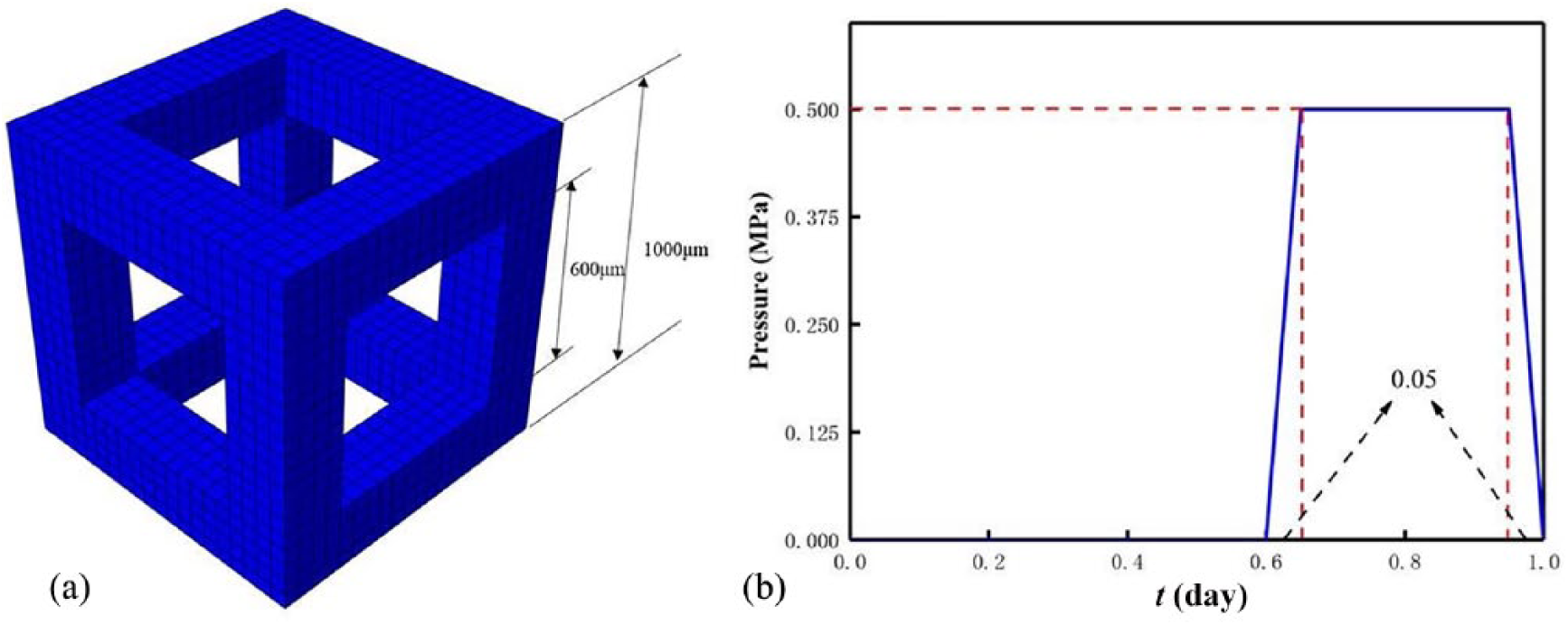
RVE of (a) a porous periodic scaffold and (b) loading trapezoidal pulse in a day.

Materials

In reality, the pore in RVE is occupied through diffused fluid after scaffold implantation. Since ISF was observed to mediate signal transduction in mechanical loading–induced remodeling,³² as stated in section “Bone formation judgment”, the pore of the RVE was assumed to be initially occupied by the ISF (5184 elements, each of them includes identical initial cell numbers, that is, 1 osteoblast and 5 osteoclasts).²² Moreover, the ISF and scaffold materials in the RVE were all assumed to be isotropic and linear elastic. It is worth mentioning that the ISF is a water-like fluid, and in fluid mechanics, the fluid is commonly treated to be incompressible.³³ Although the trabecular orientation and vessel distribution result in the macroscopic anisotropic properties of trabecular and cortical bones, respectively, the newly formed bone element in micro-scale (50 μm) on the surfaces of scaffold pillars is a trabecula-like solid material and thus could be simplified to be isotropic and linear elastic under quasi-static load.³⁴ The scaffold and bone shared the same Poisson’s ratio, which was constant in the bone in-growth process. All materials properties of the scaffold material, ISF, and bone are listed in Table 1.

Table 1.

Input parameters of the simulations.

Parameters		Value	Unit
Number of element	N	8000¹⁹	–
Young’s modulus of mature bone	E_b	20¹⁹	GPa
Young’s modulus of scaffold	E_s	5¹⁹	GPa
Poisson’s ratio of scaffold and bone	ν_s	0.3¹⁹	–
Young’s modulus of ISF	E _ISF	0.01¹⁹	GPa
Poisson’s ratio of ISF	ν _ISF	0.49¹⁹	–
Influence distance	D	0.15¹⁹	mm
Production rate of the osteoclasts	α ₁	3²²	Cells/day
Production rate of the osteoblasts	α ₂	4²²	Cells/day
Removal rate of the osteoclasts	β ₁	0.2²²	Day⁻¹
Removal rate of the osteoblasts	β ₂	0.0017²⁵	Day⁻¹
Autocrine of the osteoclasts	γ ₁₁	1.1²³	–
Autocrine of the osteoblasts	γ ₂₂	0²²	–
Paracrine of the osteoclasts	γ ₂₁	−0.5²²	–
Paracrine of the osteoblasts	γ ₁₂	1²²	–
Normalized activities of osteoclasts	k ₁	0.24%²²	Cell⁻¹ day⁻¹
Normalized activities of osteoblasts	k ₂	0.0017%²²	cell⁻¹ day⁻¹
Constant	A	10	–
Constant	B	1	–
Critical relative density	${\bar{ρ}}_{m i n}$	0.01¹⁹	–
Young’s modulus of cancellous bone	E_cb	2³⁵	GPa

Boundary condition and loading

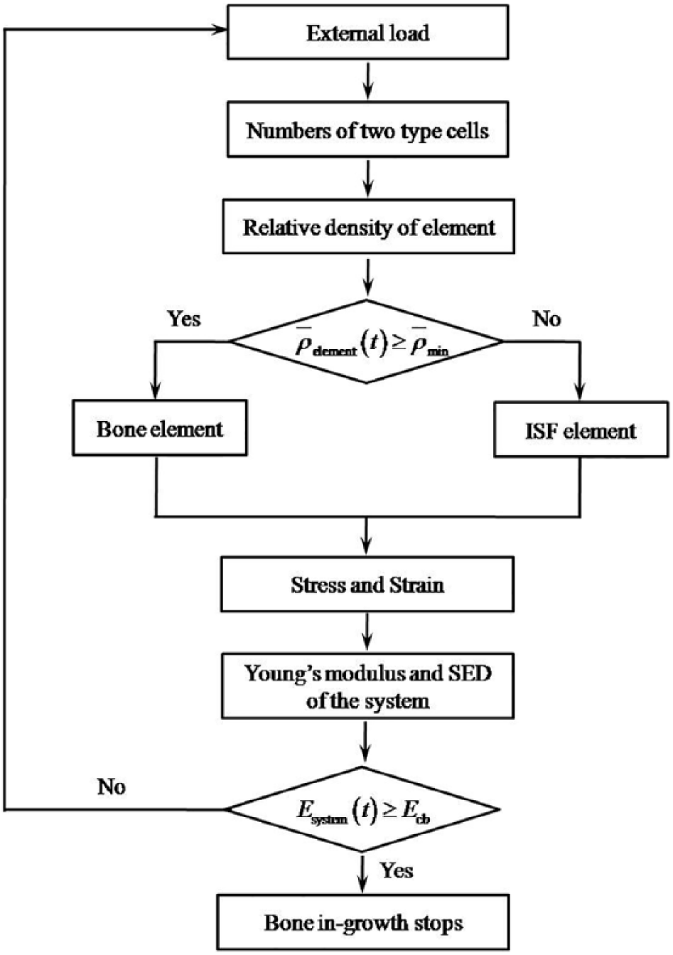
The bottom of the RVE was encastered, and the four lateral faces of the RVE were constrained to avoid translation but be able to rotate in their normal directions, and a uniformly distributed pressure was perpendicularly applied on its top surface to approximately simulate the mechanical microenvironment in body, for example, the femoral shaft. The loading history was a trapezoidal pulse in a day (Figure 1(b)). Regarding the pulse, for the sake of saving the computing cost, the RVE was quasi-statically loaded instead of being loaded in walking frequency in a day. Here, we studied three mechanical intensities (0.5, 0.7, and 1.0 MPa) and three mechanical durations (0.2, 0.3, and 0.4 day) per day¹⁹ within 200-day bone in-growth process. It is worth mentioning that the mechanical intensity was estimated by the average weight (W = 81.6 kg) and average cross-sectional area (A = 4.5 cm²) of single femoral shaft of White and Black women.³⁶ Then, the mechanical intensity σ acting on an individual femoral shaft was calculated as 0.91 MPa; moreover, considering weak mechanical stimulus at the initial stage after scaffold implantation, the intensities (0.5 and 0.7 MPa) less than 1.0 MPa were selected. The mechanical duration was estimated on the basis of the duration of daily physical activities (e.g. walking) of a normal person. The flowchart to simulate the bone in-growth is shown in Figure 2.

Figure 2.

The bone in-growing flowchart.

Simulations

The simulation was performed by coding the above flowchart into VUMAT subroutine. To solve the nonlinear models easily and efficiently, Abaqus/Explicit was employed here to guarantee the calculation convergence compared to Abaqus/Standard, and an auto-incremental time step was adopted. Moreover, the mass scaling was set to be 8 × 10⁻⁶ after several trials to balance the computing cost and the rate of convergence. For all the input parameters in the simulation, they were listed in Table 1.

Results

To study the bone in-growth into an undegradable periodic scaffold influenced by mechanical stimulus, the influences of three mechanical intensities and durations mentioned in section “Boundary condition and loading” on the BV percentage (BV/TV) of the BV to the total volume (TV = scaffold + formed bone + ISF) and the elastic SED of the scaffold–bone system are summarized and discussed.

Evolving process of bone in-growth

To validate the model, we compare the BV/TV of our simulations with that of a rat experiment, where additive manufactured porous scaffolds were modified by surface treatments and implanted into defected femoral bone of male Wistar rats³⁷ (see Figure 3). The comparison shows that the experimental results and present simulations are comparable even though there is difference between the simulating and the experimental conditions.

Figure 3.

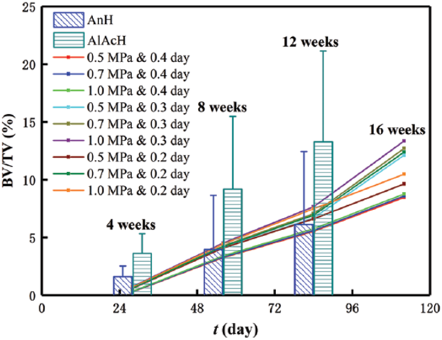
Comparison between the present simulations and animal experiments³⁷ (AnH and AlAcH are anodizing heat and alkali–acid–heat–treated scaffolds implanted in male Wistar rats at 4, 8, and 12 weeks).

Regarding the bone in-growth process, contour plots of the relative density ${\bar{ρ}}_{element} (t)$ of the case with the duration of 0.4 day and intensity of 1.0 MPa at eight time points were snapped in Figure 4. It is seen that there is no bone formation in the first two weeks (Figure 4(a)–(c)). At the end of the first month (i.e. day 30), there is a single-layered low-density bone element around the pillars (Figure 4(d)). After the first month, the single-layered low-density bone tends to mature (Figure 4(e) and (f)). Moreover, due to the greater mechanical stimulus at vertical pillars, the bone at the four vertical pillars matures faster than that at the horizontal pillars (Figure 4(g) and (h)). Following the process, the RVE is gradually filled by the newly formed bone till the system homeostasis.

Figure 4.

Snapshots of the in-growing process of bone into porous scaffold within 200 days: (a) day 7, (b) day 11, (c) day 18, (d) day 30, (e) day 47, (f) day 76, (g) day 124, (h) day 200.

In particular, the numbers of osteoclasts and osteoblasts in a randomly selected element and the scaffold–bone system (collected cells in all bone and ISF elements) are reported in Figure 5. It shows that before the homeostasis of the scaffold–bone system (i.e. cease of the bone in-growth) at day 113, the cell numbers in the element became constants in a bone cycle at around day 100,²² and the cell numbers in the system periodically varied to constants. The periodicity indicates the emergence of the newly formed bone layer where the cells were activated (i.e. at day 72, the second-layered bone element emerges), and the constant cell numbers represent a system homeostasis. Moreover, the peak of the osteoblast number always follows that of the osteoclast number, and the peak delay indicates that it takes time for signals to travel when the two activated cell types affect each other in human body.²³

Figure 5.

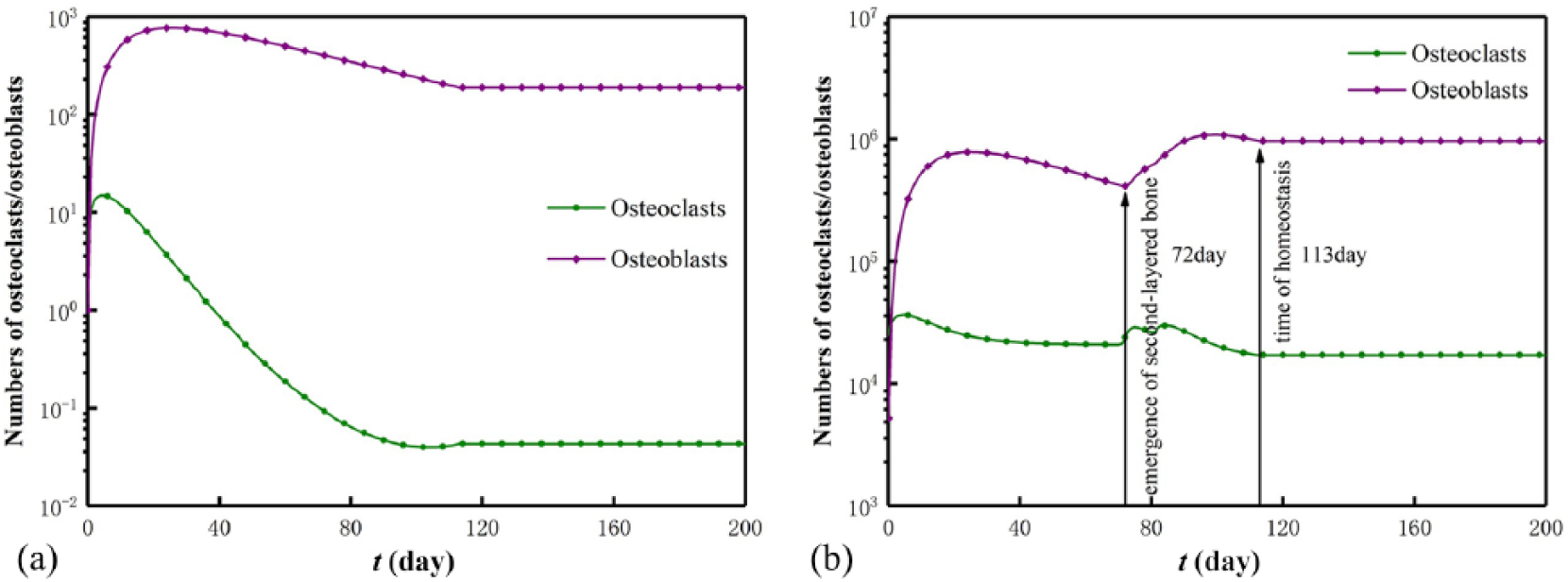
Numbers of osteoclasts and osteoblasts in (a) a remodeled element and (b) the scaffold–bone system.

Effect of mechanical intensity

Figure 6 displays the evolutions of the BV/TV and SED of the scaffold–bone system under the three mechanical intensities. Generally, as the mechanical intensity increases, the BV/TV increases before system homeostasis and is optimized after system homeostasis, while the SED of the system increases. However, for a mechanical intensity, the BV/TV increases while the SED decreases, and the decreasing SED results from the increasing system stiffness by referring SED=σ²/(2E_system(t)). Moreover, the influence of the mechanical intensity on the BV/TV is weaker than that on the SED. In particular, under durations 0.2 day (Figure 6(a)) and 0.4 day (Figure 6(e)), the BV/TV is optimized at intensity 0.7 MPa, and under duration 0.3 day (Figure 6(c)), it is optimized at both 0.5 and 1.0 MPa. Within the first 30 days, there are few low-density bone elements (see small BV/TV in Figure 6(a), (c) and (e)), and this results in the approximate constants of the SED (see Figure 6(b), (d) and (f)). In addition, the saw-like SED curve before system homeostasis results from the instable bone formation and the simulation mode of the Abaqus/Explicit in which the kinetic energy fluctuates the SED.

Figure 6.

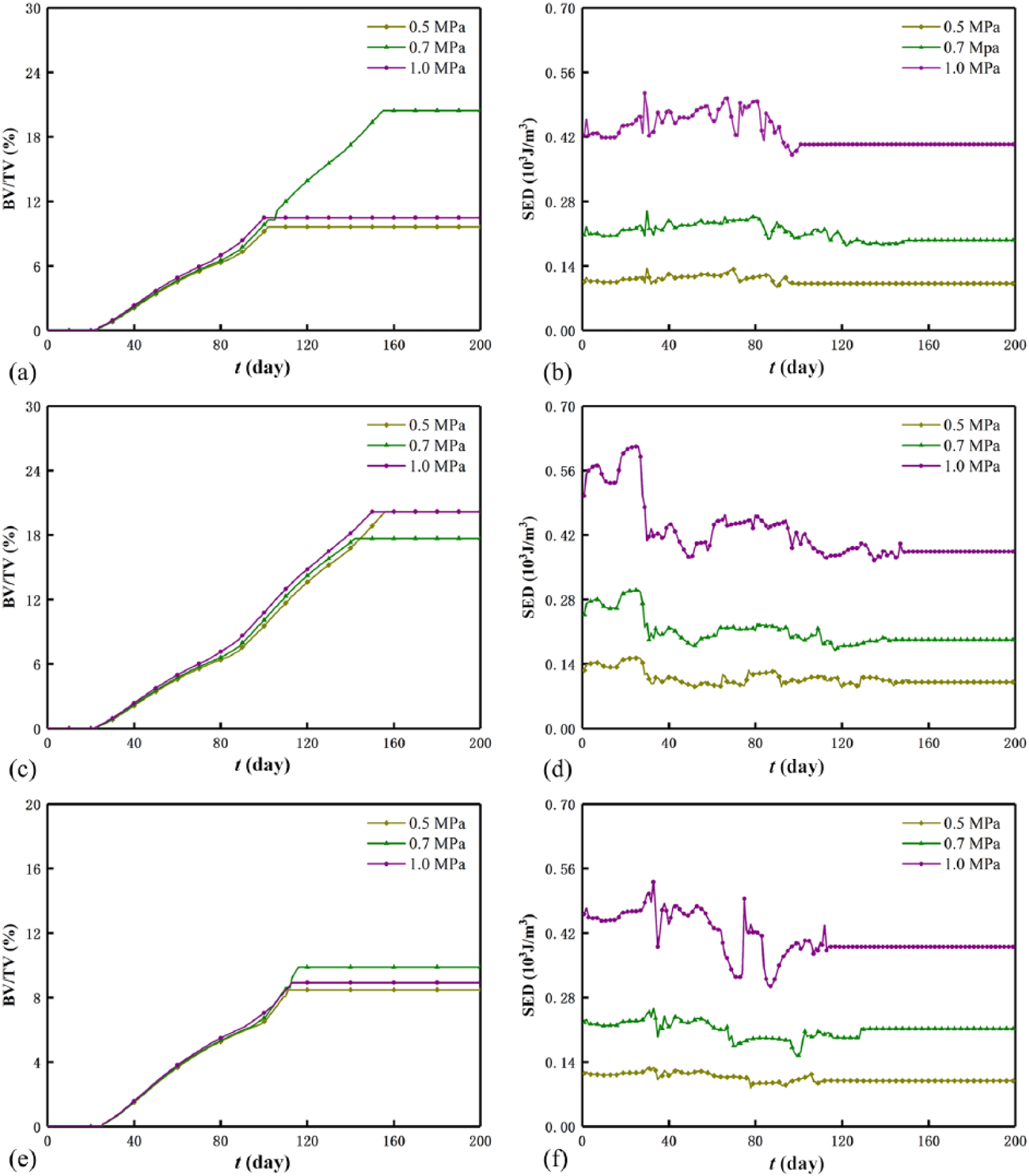
BV/TV and SED of the system under different mechanical intensities: (a) BV/TV and (b) SED for duration 0.2 day, (c) BV/TV and (d) SED for duration 0.3 day,(e) BV/TV and (f) SED for duration 0.4 day.

Effect of mechanical duration

Figure 7 displays the evolutions of the BV/TV and the SED of the scaffold–bone system under the three mechanical durations. Similar to section “Effect of mechanical intensity”, the BV/TV is optimized at 0.3 day under 0.5 MPa (Figure 7(a)) and 1.0 MPa (Figure 7(e)) after system homeostasis. For a mechanical duration, the BV/TV increases, while the SED of the system decreases. Moreover, before system homeostasis, the SED curves of the system are saw-shaped (see Figure 7(b), (d), and (f)). However, different from the mechanical intensity, in the first month, the SED of the system is optimized at 0.3 day, and this indicates that optimal bone healing requires suitable mechanical duration at the initial stage. Before system homeostasis, the cases of 0.2 and 0.3 day almost coincide with each other and are greater than the case of 0.4 day. The influence of the mechanical duration on the BV/TV is greater than that on the SED in which the three durations cannot be distinguished (see Figure 7(b), (d), and (f)). Apparently, the effect of the mechanical intensity on the SED is greater than that of the mechanical duration on the SED (see Figure 6(b), (d), and (f) and Figure 7(b), (d), and (f)).

Figure 7.

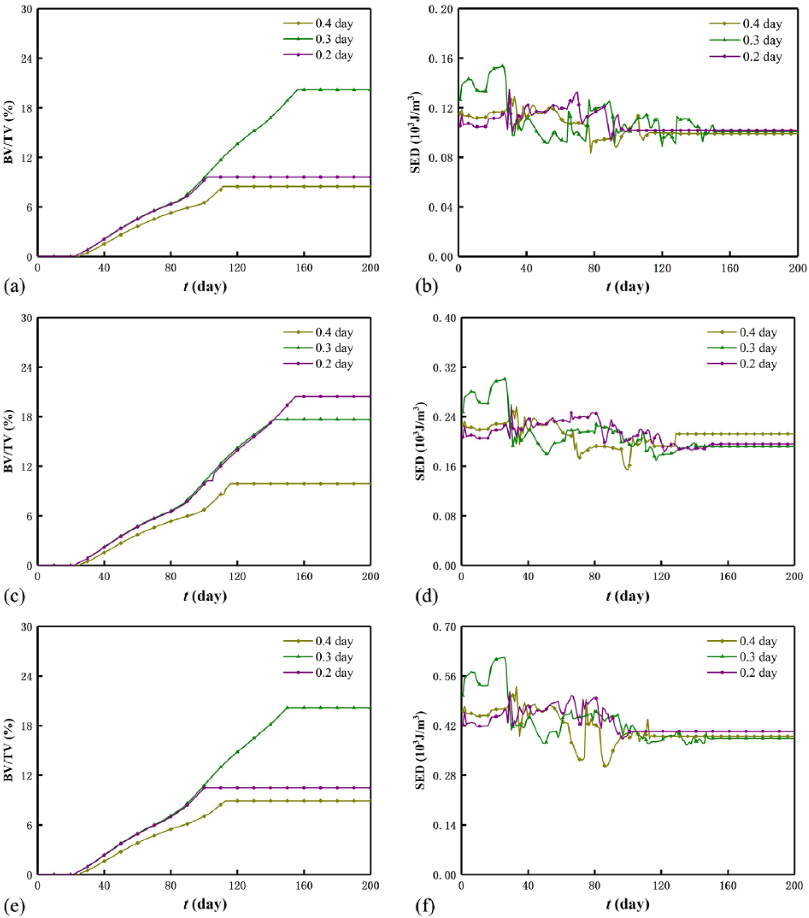
BV/TV and SED of the system under different mechanical durations: (a) BV/TV and (b) SED for intensity 0.5 MPa, (c) BV/TV and (d) SED for intensity 0.7 MPa,(e) BV/TV and (f) SED for intensity 1.0 MPa.

Comparison of all the simulations and literature

For the BV/TVs and microstrains of the scaffold–bone system after homeostasis, we compared the present results with those of cancellous bone from different human anatomical sites (Figure 8(a))³⁸ and their corresponding microstrains with the disused and healthy strain windows (Figure 8(b)).²¹ In Figure 8, the two results of the BV/TV are generally comparable, and the microstrain of the scaffold–bone system is in the healthy strain window. In detail, the BV/TV is optimized at the mechanical duration of 0.3 day in the cases of the mechanical intensities of 0.5 and 1.0 MPa (also see Figure 7(a) and (e)) and at the mechanical intensity 0.7 MPa in the case of the mechanical durations of 0.2 and 0.4 day (also see Figure 6(a) and (e)). For the mechanical durations, the cases of the mechanical intensities of 0.5 and 1.0 MPa are almost identical. Moreover, although the BV/TVs of all cases are comparable in Figure 8(a), Figure 8(b) shows that the microstrains of the system differ much, and they are all close to the lower limit of the physiological strain range (500 με - 3000 με)²⁴. This is because the microstrain of the system is determined by both applied mechanical intensity and the system Young’s modulus which correlated to the BV/TV. For instance, for the case with the mechanical intensity 1 MPa and duration 0.2 day, the BV/TV (or stiffness) of the system is smaller, but the applied intensity 1 MPa is greatest, which results in the greatest microstrain of the system. In this regard, the effect of the mechanical intensity on the microstrain is greater than that of the mechanical duration on the microstrain.

Figure 8.

(a) Bone volume percentage³⁸ and (b) microstrain of the system under mechanical stimuli. Note that in (b), HBC (healthy small and large load-bearing bones) should satisfy this criterion (MESr, MESm); MESr: 50–100 μm, disusing strain window representing the reduction of bone mass; MESm: 100–1000 μm, healthy strain window representing the increase in bone mass.²¹

Times of scaffold–bone system homeostasis

As mentioned before, when the system stiffness is greater than the regenerated bone, the stress-shielding phenomenon occurs, and the system reaches a homeostasis, and further, bone in-growth stops. Here, we also summarized the times of system homeostasis of the nine cases in Figure 9. In general, it shows that the times at homeostasis are between 3 and 5 months, which are close to those (around 110 days) in simulations^19,39 and the healing time (114 ± 10.4 days) of bone fracture in clinics.⁴⁰

Figure 9.

Homeostasis time of the scaffold–bone system of all treated cases.

Discussion

We developed a computational model of the bone in-growth into an undegradable scaffold and studied the effects of the mechanical intensity and duration on the bone in-growth by coupling the osteoblast and osteoclast activities.

Starting from the numerical method, we selected the element number 8000 on the basis of the lower density of osteocyte lacunae in natural bone and auto-incremental time step to improve the calculation efficiency. Indeed, the element number and time step influence the results. To clarify the influence, three element numbers (3375, 8000, and 64,000) and three time increments (1 × 10⁻⁴, 1 × 10⁻⁵, and auto increment) were compared based on a specific case (0.5 MPa, 0.4 day). The effect of the element numbers on the BV/TVs was shown in Figure 10(a). The increasing element number from 3375 to 64,000 diminishes the BV/TV difference (2.6% for 3375, 8.5% for 8000, and 10.4% for 64,000) and the homeostasis time difference (day 39 for 3375, day 111 for 8000, and day 105 for 64,000). This is because considering commencement of bone mineralization, we assumed when the ISF element neighboring to the scaffold surface is remodeled by 40% (BV percentage) and the adjacent ISF element is activated and starts to form. Under the assumption, the smaller sized element (or greater element number) neighboring to the scaffold surface receives greater mechanical stimulus, and a greater BV/TV is in need to meet the judgment criteria of the homeostasis of the scaffold-bone system. The effect of the time increment on the BV/TV (around 8.0%) and homeostasis time (around day 111) of the scaffold-bone system is weak, and this can be seen from Figure 10(b). In addition, the computing cost with increasing element number and time increment is greatly improved. Namely, the computing costs are around 2, 8, and 30 h for 3375, 8000, and 64,000 elements, while the cost are around 2, 8, and 20 h for the increment 1 × 10⁻⁴, the auto-increment, and the increment 1 × 10⁻⁵, respectively.

Figure 10.

Effects of the (a) element number and (b) time step on the BV/TV.

Regarding the effects of the mechanical intensity and duration, generally, in both cases, the numbers of the osteoblasts and osteoclasts in an element and the scaffold–bone system tended to be constants as the bone in-growth approached a homeostasis, and the BV/TV was optimized. The SED of the system decreased in the whole in-growth process due to the increasing stiffness of the system, and it was at the magnitude of ~10⁻⁶ J, which was less than ~10⁻⁵ J as reported in Adachi et al.³⁹ This is because that the applied pressure (2.0 MPa) in Adachi et al.³⁹ was greater than that in the present cases. A greater intensity resulted in greater BV/TV before system homeostasis. This explains the clinical observations on the greater bone mass in males than females,⁴¹ the higher bone mass in the heavier adults,^42,43 and lower bone losing rate of obese women than non-obese ones after the menopause.⁴⁴ Also, it explains that the training groups have higher BV, BMD, and bone mass than the sedentary groups, and the maximum load of mid-femur in the 4 weeks training groups is greater than that in the 8 weeks sedentary groups.⁴⁵ A final optimal BV/TV of the system exists for the mechanical stimulus. This is also consistent with the medium-intensity inhibited bone resorption and increased bone formation in young mice femur, which resulted in the improvements in the mineral density, trabecular BV, and strength.¹³ Based on the discussions, this study could propose some suggestion for clinical or rehabilitation training applications. At the initial stage (in the first month), the mechanical stimulus almost produced no bone, and this was relatively consistent with the implants at early loading time within the first two or three weeks in dogs and monkeys.⁴⁶ Moreover, considering the instability of the implants and rarely formed bone in this period, excessive rehabilitation exercise should be avoided in order to promote the osseointegration and in case of further fracture bones.

Indeed, this study has limitations because of the modeling simplification. First, the loading on the scaffold RVE is perpendicular to its surface. In reality, the loading direction is often oblique, and the oblique loads may redistribute the newly formed bone mass. Moreover, for the sake of saving computing cost, the loading in walking frequency is simply treated as a quasi-static loading mode with a single bout in a day, but the loading frequency influences the bone repair, and separated short-bout loading improves the bone structure and strength.⁴⁷ Second, ISF was considered as an incompressible solid, and the shear stress induced by the ISF was neglected. Actually, the osteoblasts and osteoclasts are believed to be also regulated by the shear stress.^17,32,48 Finally, the present model is not fully validated by experiments, and the relevant parameters are not experiment-based. Despite these limitations, this work still provides an insight to understand the bone in-growth process under the mechanical stimulus.

Conclusion

The present work proposed a mathematical model of coupling osteoclasts and osteoblasts to investigate the bone in-growth into an undegradable periodic scaffold under mechanical stimulus. The model was numerically implemented to reveal the effects of the mechanical stimulus on the bone in-growth process. Both mechanical intensity and duration optimized the bone in-growth, and the results relatively explained the experimental and clinical observations. Moreover, the model predication of the BV percentage was comparable to an experimental finding. This work could be used as a fundamental model connecting the cell level and tissue level, which provides an insight to understand the bone in-growth mechanism.

Footnotes

Declaration of conflicting interests

The author(s) declared no potential conflicts of interest with respect to the research, authorship, and/or publication of this article.

Funding

The author(s) disclosed receipt of the following financial support for the research, authorship and/or publication of this article: This study was partially supported by the National Natural Science Foundation of China (NSFC; Nos 31300780, 11272091, 11422222, 11772093, and 31470043), the Fundamental Research Funds for the Central Universities (No. 2242016R30014), and the National 973 Basic Research Program of China (No. 2013CB733800) and ARC (FT140101152). The authors also thank the School of Civil Engineering in Southeast University for the use of commercial software Abaqus.

ORCID iD

Qiang Chen

References

Gunatillake

Adhikari

Biodegradable synthetic polymers for tissue engineering. Eur Cell Mater 2003; 5(null): 1–16, discussion 16.

Weyts

FAA

Bosmans

Niesing

et al . Mechanical control of human osteoblast apoptosis and proliferation in relation to differentiation. Calcif Tissue Int 2003; 72(4): 505–512.

Rubin

Fan

Biskobing

et al . Osteoclastogenesis is repressed by mechanical strain in an in vitro model. J Orthop Res 1999; 17(5): 639–645.

Rubin

Biskobing

Fan

et al . Pressure regulates osteoclast formation and MCSF expression in marrow culture. J Cell Physiol 1997; 170(1): 81–87.

Kobayashi

Hashimoto

Miyamoto

et al . Force-induced osteoclast apoptosis in vivo is accompanied by elevation in transforming growth factor β and osteoprotegerin expression. J Bone Miner Res 2000; 15(10): 1924–1934.

Kim

et al . Impact of mechanical stretch on the cell behaviors of bone and surrounding tissues. J Tissue Eng 2016; 7: 2041731415618342.

Bhatt

Chang

Warren

et al . Uniaxial mechanical strain: an in vitro correlate to distraction osteogenesis. J Surg Res 2007; 143(2): 329–336.

Knoll

McCarthy

Centrella

et al . Strain-dependent control of transforming growth factor-β function in osteoblasts in an in vitro model: biochemical events associated with distraction osteogenesis. Plast Reconstr Surg 2005; 116(1): 224–233.

Steeve

Marc

Sandrine

et al . IL-6, RANKL, TNF-alpha/IL-1: interrelations in bone resorption pathophysiology. Cytokine Growth Factor Rev 2004; 15(1): 49–60.

10.

Liegibel

Sommer

Tomakidi

et al . Concerted action of androgens and mechanical strain shifts bone metabolism from high turnover into an osteoanabolic mode. J Exp Med 2002; 196(10): 1387–1392.

11.

Turner

Robling

AG.

Designing exercise regimens to increase bone strength. Exerc Sport Sci Rev 2003; 31(1): 45–50.

12.

Vincent

Braith

RW.

Resistance exercise and bone turnover in elderly men and women. Med Sci Sports Exerc 2002; 34(1): 17–23.

13.

Zhang

Chen

et al . The effects of different intensities of exercise and active vitamin D on mouse bone mass and bone strength. J Bone Miner Metab 2017; 35(3): 265–277.

14.

Garnero

Shih

Gineyts

et al . Comparison of new biochemical markers of bone turnover in late postmenopausal osteoporotic women in response to alendronate treatment. J Clin Endocrinol Metab 1994; 79(6): 1693–1700.

15.

Singer

Eyre

DR.

Using biochemical markers of bone turnover in clinical practice. Cleve Clin J Med 2008; 75(10): 739–750.

16.

Rattanakul

Rattanamongkonkul

Effect of calcitonin on bone formation and resorption: mathematical modeling approach. System; 2011; 3(4): 2.

17.

Adachi

Kameo

Hojo

Trabecular bone remodelling simulation considering osteocytic response to fluid-induced shear stress. Philos Trans A Math Phys Eng Sci 2010; 368(1920): 2669–2682.

18.

Tsubota

Suzuki

Yamada

et al . Computer simulation of trabecular remodeling in human proximal femur using large-scale voxel FE models: approach to understanding Wolff’s law. J Biomech 2009; 42(8): 1088–1094.

19.

Shi

Chen

Pugno

et al . Effect of rehabilitation exercise durations on the dynamic bone repair process by coupling polymer scaffold degradation and bone formation. Biomech Model Mechanobiol 2018; 17(3): 763–775.

20.

Huiskes

Weinans

vanRietbergen

The relationship between stress shielding and bone resorption around total hip stems and the effects of flexible materials. Clin Orthop Relat Res 1992; 274: 124–134.

21.

Frost

HM.

A 2003 update of bone physiology and Wolff’s Law for clinicians. Angle Orthod 2004; 74(1): 3–15.

22.

Komarova

Smith

Dixon

et al . Mathematical model predicts a critical role for osteoclast autocrine regulation in the control of bone remodeling. Bone 2003; 33(2): 206–215.

23.

Chen-Charpentier

Diakite

A mathematical model of bone remodeling with delays. J Comput Appl Math 2016; 291: 76–84.

24.

Tang

Wang

et al . The physiological response of osteoblasts to a gradiently increased stretching. Acta Bioph Sin 2003, 19(1): 88–91. (In Chinese).

25.

Hambli

Connecting mechanics and bone cell activities in the bone remodeling process: an integrated finite element modeling. Front Bioeng Biotechnol 2014; 2: 6.

26.

Schulte

Zwahlen

Lambers

et al . Strain-adaptive in silico modeling of bone adaptation—a computer simulation validated by in vivo micro-computed tomography data. Bone 2013; 52(1): 485–492.

27.

Marcus

Normal and abnormal bone remodeling in man. Annu Rev Med 1987; 38(null): 129–141.

28.

Gibson

LJ.

The mechanical behaviour of cancellous bone. J Biomech 1985; 18(5): 317–328.

29.

Currey

JD.

The effect of porosity and mineral content on the young’s modulus of elasticity of compact bone. J Biomech 1988; 21(2): 131–139.

30.

Hannah

Thomas

CDL

Clement

et al . Bimodal distribution of osteocyte lacunar size in the human femoral cortex as revealed by micro-CT. Bone 2010; 47(5): 866–871.

31.

Ding

Hvid

Quantification of age-related changes in the structure model type and trabecular thickness of human tibial cancellous bone. Bone 2000; 26(3): 291–295.

32.

Hillsley

Frangos

(1994) Bone tissue engineering: the role of interstitial fluid flow. Biotechnol Bioeng 43(7): 573–581.

33.

Mak

AF.

The apparent viscoelastic behavior of articular cartilage—the contributions from the intrinsic matrix viscoelasticity and interstitial fluid flows. J Biomech Eng 1986; 108(2): 123–130.

34.

Huiskes

On the modelling of long bones in structural analyses. J Biomech 1982; 15(1): 65–69.

35.

Hodgskinson

Currey

JD.

Young’s modulus, density and material properties in cancellous bone over a large density range. J Mater Sci 1992; 3(5): 377–381.

36.

Nelson

Barondess

Hendrix

et al . Cross-sectional geometry, bone strength, and bone mass in the proximal femur in black and white postmenopausal women. J Bone Miner Res 2000; 15(10): 1992–1997.

37.

Yavari

van der Stok

Chai

et al . Bone regeneration performance of surface-treated porous titanium. Biomaterials 2014; 35(24): 6172–6181.

38.

Ulrich

van Rietbergen

Laib

et al . The ability of three-dimensional structural indices to reflect mechanical aspects of trabecular bone. Bone 1999; 25(1): 55–60.

39.

Adachi

Osako

Tanaka

et al . Framework for optimal design of porous scaffold microstructure by computational simulation of bone regeneration. Biomaterials 2006; 27(21): 3964–3972.

40.

Heckman

Ryaby

McCabe

et al . Acceleration of tibial fracture-healing by non-invasive, low-intensity pulsed ultrasound. J Bone Joint Surg Am 1994; 76(1): 26–34.

41.

Felson

Zhang

Hannan

et al . Effects of weight and body mass index on bone mineral density in men and women: the Framingham study. J Bone Miner Res 1993; 8(5): 567–573.

42.

Reid

Plank

Evans

MC.

Fat mass is an important determinant of whole body bone density in premenopausal women but not in men. J Clin Endocrinol Metab 1992; 75(3): 779–782.

43.

Douchi

Yamamoto

Oki

et al . Relationship between body fat distribution and bone mineral density in premenopausal Japanese women. Obstet Gynecol 2000; 95(5): 722–725.

44.

Dawson-Hughes

Shipp

Sadowski

et al . Bone density of the radius, spine, and hip in relation to percent of ideal body weight in postmenopausal women. Calcif Tissue Int 1987; 40(6): 310–314.

45.

Notomi

Okimoto

Okazaki

et al . Effects of tower climbing exercise on bone mass, strength, and turnover in growing rats. J Bone Miner Res 2001; 16(1): 166–174.

46.

Szmukler-Moncler

Salama

Reingewirtz

et al . Timing of loading and effect of micromotion on bone -dental implant interface: review of experimental literature. J Biomed Mater Res 1998, 43(2): 192–203.

47.