Sage Journals: Discover world-class research

Abstract

Interest in continuous psychophysical approaches as a means of collecting data quickly under natural conditions is growing. Such approaches require stimuli to be changed randomly on a continuous basis so that participants can not guess future stimulus states. Participants are generally tasked with responding continuously using a continuum of response options. These features introduce variability in the data that is not present in traditional trial-based experiments. Given the unique weaknesses and strengths of continuous psychophysical approaches, we propose that they are well suited to quickly mapping out relationships between above-threshold stimulus variables such as the perceived direction of a moving target as a function of the direction of the background against which the target is moving. We show that modelling the participant in such a two-variable experiment using a novel “Bayesian Participant” model facilitates the conversion of the noisy continuous data into a less-noisy form that resembles data from an equivalent trial-based experiment. We also show that adaptation can result from longer-than-usual stimulus exposure times during continuous experiments, even to features that the participant is not aware of. Methods for mitigating the effects of adaptation are discussed.

Keywords

Bayesian inference data analysis continuous psychophysics induced motion adaptation

Introduction

Trial-based methods have been a mainstay in psychophysics since its inception over 160 years ago (Prins et al., 2016; Wichmann et al., 2018). Recently, however, there has been a renewed interest in continuous psychophysical approaches that call for the sustained, active participation of the person taking part in the experiment (Ambrosi et al., 2022; Bonnen et al., 2015; Burge & Cormack, 2020; Grillini et al., 2021; Huk et al., 2018; Kuo et al., 2017; Lakshminarasimhan et al., 2020; Straub & Rothkopf, 2022).

This renewed interest is a result of various factors: the capacity for rapid response sampling by fast computers; the ability to adjust stimuli in real-time based on participant responses; the natural extension of research interests from highly controlled lab scenarios to naturalistic environments and behaviors; and advances in Virtual Reality and other immersive systems enabling realistic simulation of more natural environments. If proven reliable, continuous psychophysics approaches would offer several advantages. They would allow for the study of human perception and behavior under more natural conditions, would provide more engaging experimental experiences which would reduce effects associated with participant fatigue and distraction, and the data could be collected in a fraction of the time needed for trial-based methods (Huk et al., 2018).

An issue that needs to be addressed if continuous methods are to play a significant role in the field of psychophysics is data reliability. There are at least two extra sources of variability inherent to a continuous approach where stimuli are continually varied randomly and participants respond concurrently.

There is high uncertainty associated with the stimulus as it must be varied continuously and randomly in order to avoid guessing of future stimulus states.

There is greater variability associated with the action system. Rather than the constrained number of response options intrinsic to trial-based experiments (often binary) and a generous amount of time to respond, participants are forced to respond quickly in a continuous experiment and there is a continuum of response options.

Is there a way to utilize the potential benefits of a continuous approach while addressing reliability concerns? Data reliability was bolstered in the case of trial-based approaches with the advent of signal detection theory (SDT, Green & Swets, 1966) because it provides a reliable means of accounting for, and making use of, the variability that is inherent in trial-based data. This is accomplished by explaining the source of that variability and how it relates to key internal states in the observer (Swets et al., 2001; Szalma and Hancock, 2015).

A continuous equivalent of SDT is needed that accounts for the variability in continuous experiments (see Straub & Rothkopf, 2022: for a discussion of the inability of SDT to model participants in continuous experiments). In the present paper, we discuss a novel model of a participant in a continuous experiment that accounts for the noise in the participant’s responses. We show how it can be used to produce data that is as low in unexplained variability as that obtained from a trial-based experiment.

Before presenting the model, it is important to define a realm in which continuous psychophysics could play a useful role, as that will determine the general shape of the appropriate model. Just like the earliest proposed continuous psychophysics method called the Method of Adjustment (Fechner, 1860), modern continuous methods are unlikely to be well-suited for determining precise detection thresholds and discrimination thresholds (or “just noticeable differences”) because of the variability inherent in these approaches (Blackwell, 1952; Farell & Pelli, 1999). Accordingly, recent continuous approaches have been employed successfully for studies that don’t involve determining thresholds. Examples include the estimation of sensory noise while a participant continuously tracks the position of a well-above-threshold Gaussian blob moving on a plane (Bonnen et al., 2015; Straub & Rothkopf, 2022), the measurement of internal noise while a participant tracks an object moving through three-dimensional (3D) space (Bonnen et al., 2017), the perceived motion of an object in 3D space as a function of the delay between left and right eye images (Burge & Cormack, 2020), the approximation of internal sensory and action noise while a participant corrects for random changes in the numerosity and area of a cloud of dots (Ambrosi et al., 2022) and tracing the temporal evolution of a contrast-induced speed bias (Patricio Décima et al., 2022).

A currently unexplored application for continuous psychophysics is the fast exploration of relationships between two above-threshold stimulus variables. In principle, a continuous method could be applied to quickly map the relationship for any study of the effect of one above-threshold variable on another in a psychophysical study. Examples include the effect of orientation of a high contrast surrounding grating on the perceived contrast of a central grating, the perceived tilt of a vertical bar as a function of the proximity of a pair of surrounding tilted bars, the effect of the position of a visual stimulus on the perceived location of an auditory stimulus, and perceived driving speed as a function of proximity to guard rails.

In this paper, we examine how the direction of a moving background affects the perceived direction of a moving target. It has long been known that when a target (moving or not) is placed against a background that moves, the target will perceptually inherit a motion vector opposite to that of the background (Duncker, 1929; Farrell-Whelan et al., 2012; Reinhardt-Rutland, 1988). The effect is referred to as Induced Motion. For example, when a red target circle moves vertically upwards on a computer screen against a background blue frame moving to the right, the target will appear to move upwards, as expected, but also to the left, in a direction opposite to the motion of the background.

In our example experiment, we continuously varied the direction of the background in a random manner so that participants could not guess what direction it would move in next, and asked participants to adjust the target so that it always appeared to move vertically. The difference between the actual target direction and its nominal perceived direction (vertical) was taken as the size of the induced motion effect for a given background direction (Falconbridge et al., 2022; Farrell-Whelan et al., 2012; Zivotofsky, 2004). Participants in the experiment thereby engaged in what may be termed a continuous-correction task. This is similar to a traditional above-threshold nulling task, but where an aspect of the stimulus that affects perception is continuously and randomly perturbed.

We now briefly introduce a Bayes-optimal model of an experimental participant which we call the Bayesian Participant (BP) model. The BP is assumed to have an internal generative model of the processes occurring in the outside world that produce the continuous stimuli experienced. The BP updates estimates of world states using two sources of information: Its own predictions about how the world will change, and new sensory data. The weight given to each is determined by the estimated variance within each information channel. The weights are Bayes-optimal.

The estimates of world states so produced are compared with states representing the participant’s goal and any discrepancies between the two drive participant action. In the case of our example experiment, the world variable of interest was the direction of motion of a target. The internal estimate of that direction corresponds with the perceived direction experienced by a participant. If this direction is left or right of vertical then an ideal correcting action is planned. Planned actions are those that are expected to produce perceptions that are more aligned with the goal based on the BP’s model of its own action system and how its actions change the world. The difference between the planned actions and the actual actions of a participant is attributed to additive noise in the action system.

This is one sense in which our BP model differs from a Kalman filter. Although they are similar in that both estimate hidden world states using a Bayesian inference framework, the BP model goes further by estimating appropriate actions for meeting a goal. We will see that another sense in which they differ is that the BP model assumes constant internal and external noise variance during experimental sessions.

A schematic representation of the BP in the above context is sketched in Figure 1. We outline the BP model in more detail in the next section and provide mathematical details in Appendix A.

Figure 1.

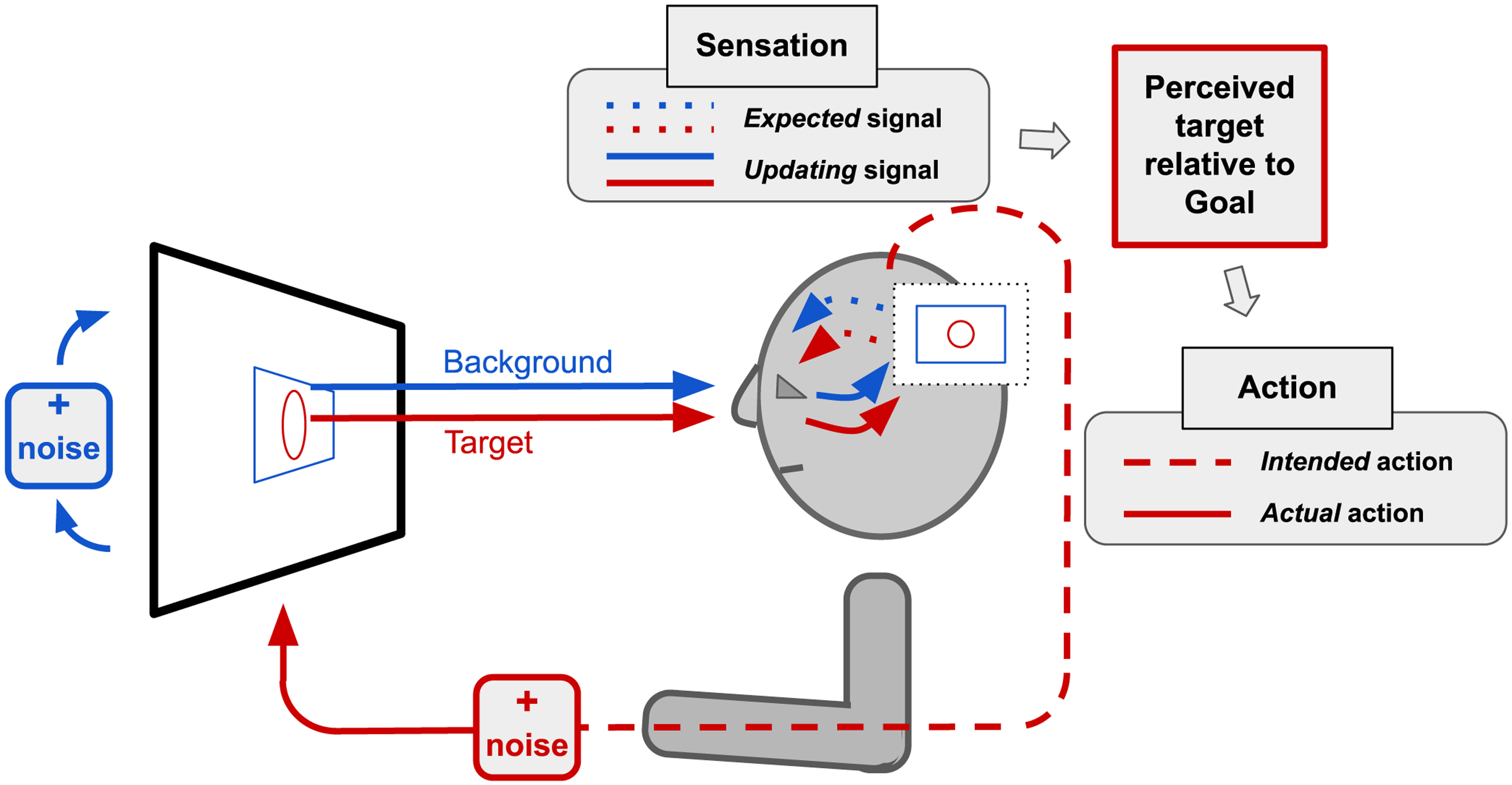
Schematic representation of our Bayesian Participant taking part in a continuous-correction experiment. The background (blue) direction is randomly perturbed (“+ noise”) at regular intervals and the target (red) direction is continuously adjusted by the participant in an effort to keep the perceived target direction close to a goal state. Estimates of world states (“Sensation”) and choices about how to correct the target (“Action”) are Bayes-optimal.

Our model has been designed to aid in the analysis of data from continuous experiments. The way it does so will now be described.

The first assumption for our data analysis approach is that the aim of a two-variable experiment to which our approach is applied is to probe the relationship between the dependent and independent variables. Recall that the dependent variable is the aspect of the stimulus that is altered by the computer, and the dependent variable is the aspect of the stimulus that is under the control of the participant. Updates to the second are made in response to the computer-driven adjustments to the first.

Such an experiment will produce data sets representing the dependent and independent variables, but the data will be corrupted by the extra sources of data variability outlined above.

Our second assumption is that there exists a mechanism in the brain of the participant that is the basis for the relationship between the dependent and independent data values. This mechanism can be thought of as a function; it takes current dependent and independent variable values and produces a “percept” for the dependent variable. In turn, this percept drives actions that determine future dependent values. We label this function $f$ . We assume that this function $f$ operates independently of the experimental approach; it will produce the same results whether the participant is in a trial-based experiment or a continuous experiment.

The differences between trial-based and continuous results lie in the sensory processes leading up to $f$ and the action processes that follow $f$ , not $f$ itself. In a continuous experiment, the sensory system will suffer from the extra sources of perceptual variability outlined above and the action system will suffer from the extra sources of action variability outlined above. If these extra sources of variability can be accounted for, it should be possible to see clearly the operation of the function $f$ by knowing its inputs and the percepts it produces at any one time. These function inputs and outputs should be the same as those in an equivalent trial-based experiment.

Our BP model makes precise predictions about how the dependent and indpendent variables will be altered by a participant’s sensory system during a continuous experiment to produce inputs to $f$ . It also makes precise predictions about how the dependent variable percepts, which are the outputs of $f$ , will lead to actions. This allows an experimenter to take the actual dependent and independent variable data sets and trace them downstream to find model estimates of inputs to the function $f$ . It also allows an experimenter to trace the dependent variable data upstream through the action system to the model outputs of the function $f$ that drove the actions of the participant. In this way, an experimenter can produce new data sets representing the dependent and independent inputs to $f$ as well as the dependent outputs.

These new data sets are ideal because they are the values produced by a Bayes-optimal perception-action system. Our BP is similar to an ideal observer (Geisler, 2003), but with the addition of an “ideal” action system; one where the actions are optimal in a Bayesian sense. What we show below is that the ideal data sets produced using our BP model are similar to data sets from a more controlled trial-based experiment.

In the next section, we describe our BP model in enough detail that readers should be able to follow descriptions of its application in later sections. In the ‘Application of the BP Model to Induced Motion' section we detail our induced motion experiment and the application of the BP model to analyze the data from that experiment. In the ‘Comparing Results to Trial-Based Results' section we compare our results to those from an equivalent trial-based experiment conducted previously in our lab. The comparison is promising but it highlights a potential danger associated with continuous psychophysics approaches in general—the issue of adaptation. In our first experiment, participants were exposed to target motion for a prolonged period in one prevailing nonvertical direction. Even though the participants were unaware of this nonvertical component it appeared to cause adaptation in lower-level neurons which led to the participants adjusting the target more and more towards the prevailing nonvertical direction. Methods for controlling the impact of adaption are presented and shown to be effective. The paper closes with a short summary and discussion in the final section.

BP Model

The schematics in Figures 2 and 3 depict both a continuously varying stimulus and a BP responding to the changing stimulus in greater detail than does Figure 1. Figure 2 uses words to describe the stages, employing our experiment as an example, and Figure 3 contains the same stages represented in equation form. Arrows indicate loops and flows driving the stimulus and participant behavior.

Figure 2.

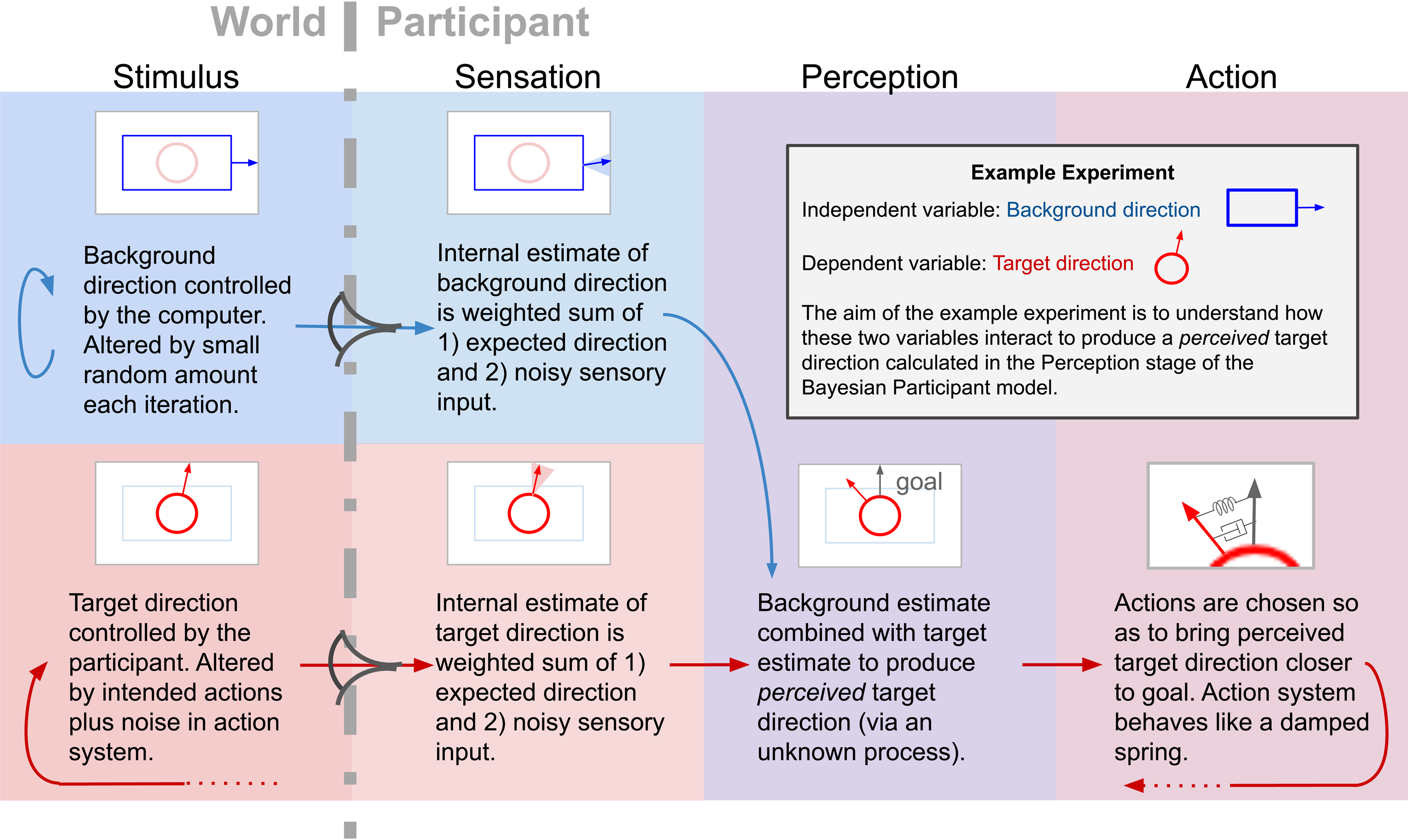
BP model in words. The background (blue) and target (red) update procedures are broken down into stages; changes to stimulus properties (World), the transduction of those properties into sensory states, the estimation of world stimulus properties based on sensations and an internal model of the external world (Sensation), the combining of background and target estimates to produce target perceptions (Perception) and the instigation of actions that drive target perceptions closer to goal states (Action).

Figure 3.

BP model in equations. Here, the words in Figure 2 have been replaced with equations. These equations describe all changes that occur at each iteration, both in the world and in the BP. See the text for an explanation and Appendix A for a deeper mathematical discussion along with the derivation of these equations.

As shown in the figures, the BP may be broken down into three stages. We have labeled these stages Sensation, Perception, and Action but note that these are lose categorizations; used only for the purpose of stage separation. Each of these stages will be treated individually below after the stimulus generative process has been described.

Stimulus

The stimulus is composed of (at least) two parts one is controlled by the computer and the other is controlled by the participant. The variables representing the states of these components are labeled the “independent” and the “dependent” variables respectively. The word “dependent” is used because the perception of this variable is a function of the “independent” variable. The independent variable is labeled $x$ in Figure 3 and the dependent is labeled $y$ .

The independent variable is randomly perturbed at each iteration; stepped by a small amount, $μ$ , where $μ$ is selected from a Gaussian distribution with a mean of zero and variance $σ_{μ}^{2}$ . The dependent variable is updated by the actions of the participant. These actions are the sum of an intended component, $a$ , and zero-mean Gaussian noise, $λ$ .

Sensation

In the first stage of the BP model, denoted “Sensation” in Figures 2 and 3, estimates of $x$ and $y$ are inferred. These are labeled $\hat{x}$ and $\hat{y}$ respectively. Inference is based on Baye’s theorem. This stage employs a model of the dynamic behavior of the external world. This model makes predictions about future world states and has “expectations” about the future sensations that will flow from those predicted states.

The sensory expectations of the perceptual system are compared to the sensory data arriving from the world. The sensory data are labeled $X$ and $Y$ and are just noisy versions of $x$ and $y$ . If the prediction and sensory data differ, the internal estimate of the relevant external variable is updated. For the independent variable the statistically accurate expectation is that the sensory input will not change as changes to $x$ in the world are random with a mean of zero. For the dependent variable, the statistically accurate expectation is that the previous state will be updated by the known actions of the participant.

The actual and expected sensory states are weighted by a weighting factor, $k$ , and $1 - k$ respectively. This factor is a simple function of the known variance in the sensory system and the estimated variance in the world variable. Calculation of $k$ is detailed in Appendix A.

Perception

The estimates of world states are combined in the Perception stage of the model where a “percept” of the dependent variable is formed based on an interaction between the estimates of the dependent and independent variables. This interaction between the independent and dependent variables is not known and the experiment is designed to probe it. For example, in our experiment, we examine target direction perception as a function of the current background and target directions. The internal estimate of target direction is labeled $\hat{y}$ , perceived target direction (nominally vertical) is labeled $\tilde{y}$ and the internal estimate of background direction is labeled $\hat{x}$ .

The interaction is described by the unknown function labeled $f (\hat{x}, \hat{y})$ in Figure 3 which is a specific example of the function $f$ used more generally in this paper. The inputs to this function are the estimates $\hat{x}$ and $\hat{y}$ from the previous stage of the BP model. The output is $\tilde{y}$ and represents the “perceived” value of the dependent variable.

The entire data analysis is centered on this stage of the model. The aim is to determine $\hat{x}$ and $\hat{y}$ from the raw data $x$ and $y$ and to determine $\tilde{y}$ from $y$ based on a model of the actions of the participant. Calculating the inputs and outputs of $f (\hat{x}, \hat{y})$ in this way allows us to determine the properties of this function experimentally.

Action

The action system is based on the commonly used damped spring model of actions by human hands (André et al., 2014; Borst & Indugula, 2006; de Lussanet et al., 2002; Hollerbach, 1981; Speich et al., 2005). The function of the action system is to correct deviations of the perceived dependent variable from some goal state through the use of two forces. The first is a spring restoring force that “pulls” the perceived dependent variable towards the goal and the second is a damping force that slows movements to minimize overshooting.

The action system has two parameters: A spring constant $b$ and a damping constant $c$ . Note that a time lag $Δ t$ is included in the damped spring expression to account for the fact that responses to stimuli occur sometime after the driving stimulus is presented. The actions produced by the damped spring system are termed “intended actions” to distinguish them from the actual actions of the participant which have Gaussian noise, denoted $λ$ , added to them. We attribute the noise to unexplained variability introduced by the physical system that implements the actions.

The actions are assumed to be driven by discrepancies between perceptions and goal states for the dependent variable. This shapes the experimental protocol. In our experiment, rather than have participants simply report the direction of the target stimulus under changing background conditions, they were instructed to adjust the target direction to meet a goal.

We propose that most phenomena involving relationships between two different stimulus properties can be studied using experiments where participants are tasked with adjusting some aspect of the stimulus to meet a goal. But, some phenomena may be more amenable to a tracking task where participants simply report the perceived state of some aspect of the stimulus. Reporting can take many forms, for example, pointing or moving a cursor on a screen to indicate the perceived position of some aspect of the stimulus. In Appendix D it is shown that our BP model can be adjusted slightly to be used in such experiments. This allows for target-tracking experiments like those used in most continuous psychophysics experiments to date (Ambrosi et al., 2022; Bonnen et al., 2015; Burge & Cormack, 2020; Kuo et al., 2017; Grillini et al., 2021; Huk et al., 2018; Lakshminarasimhan et al., 2020; Straub & Rothkopf, 2022).

Note that we have presented the action system independent of any Bayesian considerations. In Appendix C we show how the action system relates to Bayesian Decision Theory (BDT). Briefly, BDT assumes actions are chosen whose outcomes maximize utility. Utility is a measure of the worth of outcomes and takes energetic costs and the value of the outcomes into account (Körding & Wolpert, 2006). Using our experimental data we show that utility is approximately maximized by assuming the actions are a product of a damped-spring action system.

Application of the BP Model to Induced Motion

In this section, we show how the Bayesian Participant model can be applied to a continuous version of an induced motion experiment. The independent variable, $x$ , is the background direction and the dependent variable, $y$ , is the target direction set by participants in an effort to make the target direction appear vertical. In our first experiment, this direction was generally up and to the right in order to cancel the leftward motion induced by the background that always has a rightward component of motion. A stimulus screenshot is shown in Figure 4. A movie of the stimulus is in Supplemental Materials 1.

Figure 4.

Screenshot of an example stimulus. The target consisted of 30 so-called “Gabor patches” arranged on a ring. Each stripy pattern within each stationary patch drifted in a manner consistent with the global target speed and direction. The remaining patches constituted the background. The patterns in these patches, likewise, drifted in a manner consistent with the global motion of the background. See example stimulus movie in Supplemental Materials 1.

The target consisted of 30 Gabor patches arranged in a circle centered on the middle of the display. Each Gabor remained in place but the pattern within drifted perpendicular to the orientation of its stripes at a speed that was consistent with the global velocity of the target object. The background consisted of the remaining 40 Gabors and the corresponding drift of each was consistent with the global background velocity.

Participants viewed this stimulus on a monitor and were asked to fixate as well as possible on the center of the display area while they continuously adjusted the target direction with a mouse to make it appear to move upwards. Fixating centrally is the best way to judge target direction as the nature of the stimulus calls for the integration of many differently oriented local patterns to get a sense of the global speed and direction of the target circle. This is because it is only possible to see a single component of the target motion by looking at a single Gabor patch, namely the component orthogonal to the Gabor’s stripes. This is because motion along the stripes is not visible as there is no texture to indicate such motion. One needs to integrate across at least two different component directions to get a sense of the 2D global target motion; the more such signals there are, the less noisy the global percept becomes. Global motion produced in this way is referred to as Global Gabor (Amano et al., 2009) or Dynamic Global Gabor motion (Rider et al., 2009).

The background elements also carried a global motion signal. The background direction underwent a random walk which affected the perceived target direction necessitating continuous corrections by the participant in order to keep the target perceptually moving vertically. Stimulus details are given in Appendix E.

The experiment described here is a continuous version of a trial-based experiment conducted previously in our lab (Falconbridge et al., 2022). The reasons for using a Global Gabor stimulus are presented in the original study. The data from the trial-based experiment, presented below as a comparison to our continuous experiment, took about $3.5$ hours per individual to collect and produced $20$ data points per individual. By way of comparison, the continuous method produced about $9$ equivalent data points, based on about $2000$ measurements, for each two-minute session. With this method, the same $20$ data points can be collected in just over four minutes. This represents a dramatic reduction in testing time.

Training Session

A training session was employed in order to familiarize participants with their task and to tune the model to each participant. The training session involved a small 2D Gaussian luminance “blob” (a 2D Gaussian luminance profile) positioned on the outer rim of the circular stimulus area performing a random walk. The walk consisted of stepping $10^{\circ}$ either clockwise or anticlockwise with equal probability, every five seconds.

The goal of the participant was to direct the target’s motion towards the center of the blob. As we wanted our participants to get used to a moving background, during the training sessions we had each randomly oriented background Gabor element move at a random speed creating a sense of movement in the background but without any coherent global direction.

The target direction was varied by the participant using a mouse where rightward movement produced a clockwise change in direction and leftward movement an anticlockwise change. Training sessions lasted $130$ seconds but the first $10$ seconds of data was not analyzed.

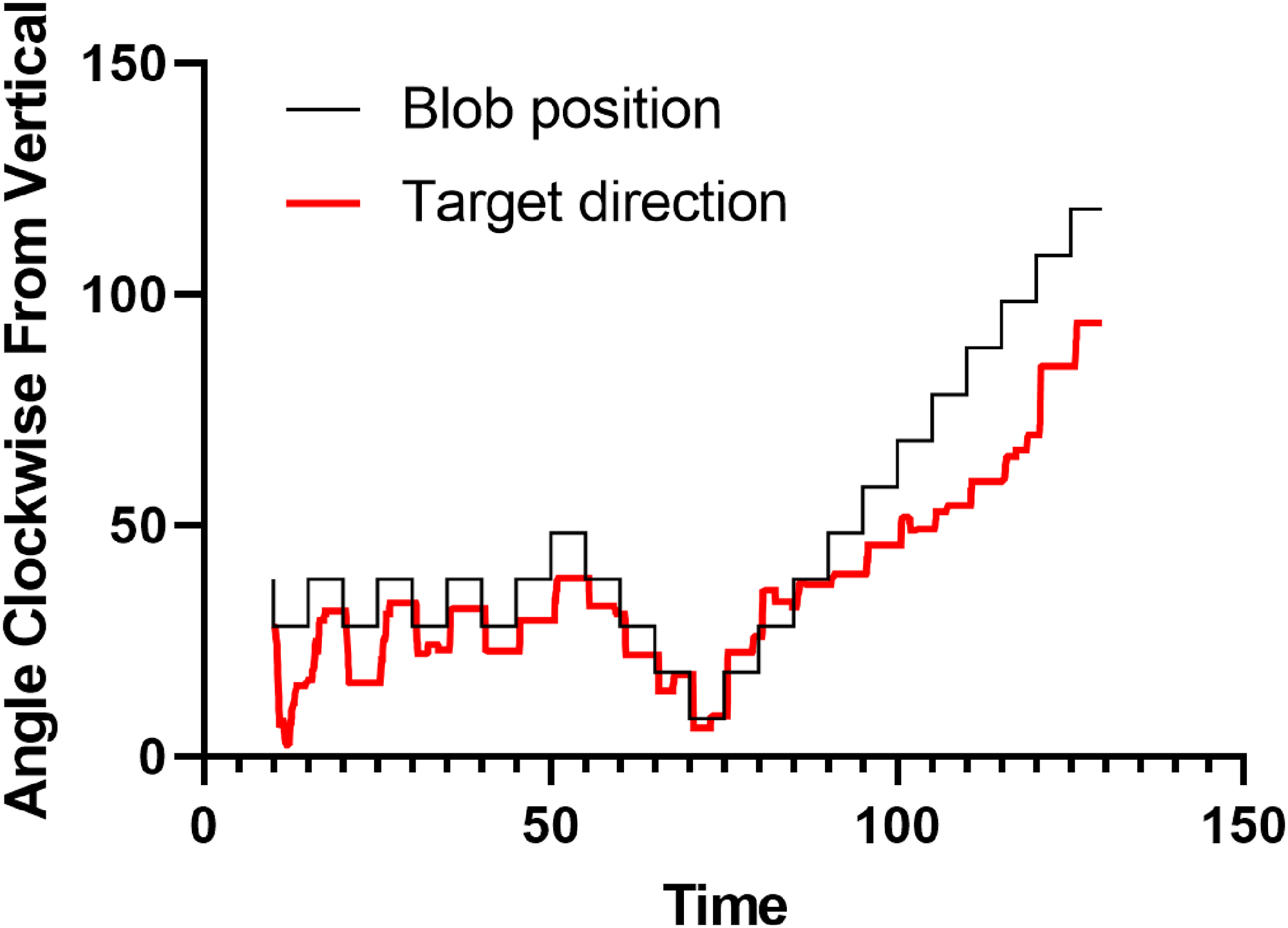
Figure 5 shows the last $120$ seconds of an example time series for the computer-generated blob direction and participant-driven target direction for participant ED.

Figure 5.

Example time series for blob angular position and target direction during a training session. The participant’s task was to adjust the target direction so that it appeared to move towards the blob which was positioned 17 degrees from fixation outside of the background display area. Participant ED.

As expected, the target data lags behind the blob data, the transitions lack the same square step profile as the blob steps, and the steps end on final values that are some distance from the actual blob values. The average time lag for a response was $0.41 s$ and the variance of the difference between the blob and target data at the end of each blob direction step was $1.6 \deg^{2}$ . These constitute estimates of $Δ t$ and $σ_{ω}^{2}$ ( $= σ_{ψ}^{2} = σ_{ϕ}^{2}$ ), respectively (see Figure 3 and equations A.12, A.2, A.8, and A.11 respectively).

To get a sense of how participants responded on average to a single blob step, the responses to each blob step were aligned, rectified to make all steps in the same direction for comparison, and averaged. Figure 6 shows individual rectified responses to steps, the average step response and the result of fitting the damped-spring model in the last panel of Figure 3 (equation A.13) to the average step response for two participants.

Figure 6.

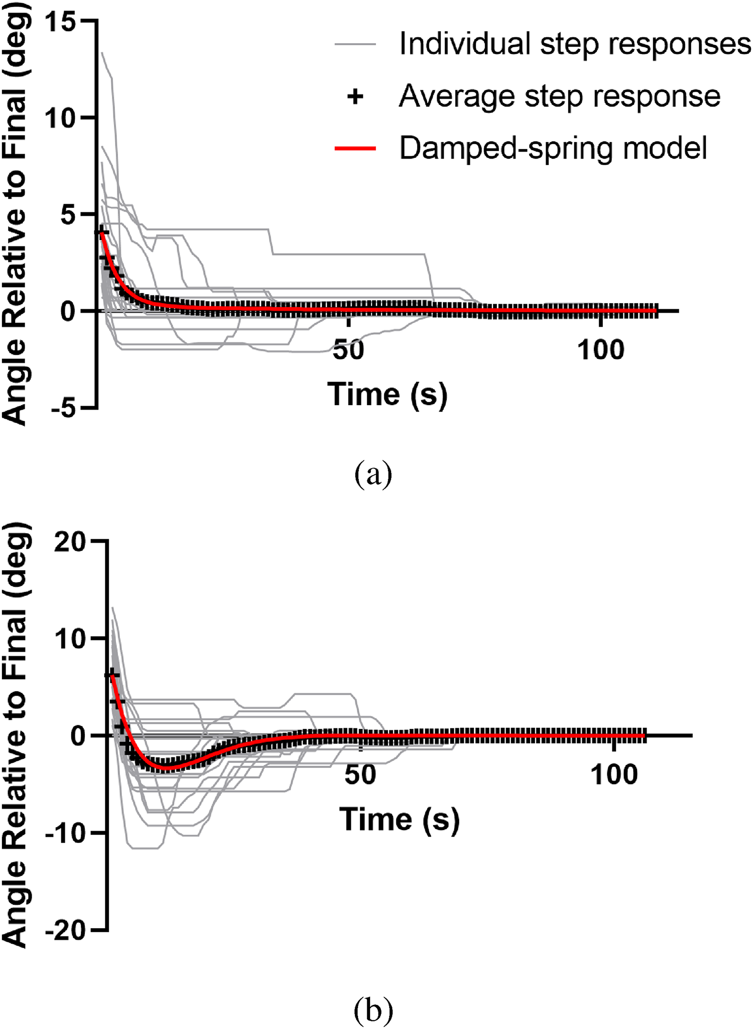
Rectified responses to steps for two participants. Top: Target direction values following the blob steps depicted in Figure 4 for participant ED. Individual responses to a blob step (light gray), the average response (+) and the damped spring model (red) are shown. Bottom: Equivalent step responses for participant MF for comparison. MF’s optimal spring model has a relatively lower damping constant leading to the overshooting seen in the figure.

The optimal spring constants for ED were $b = 0.375$ and $c = 0.008$ . For comparison, they were $b = 0.272$ and $c = 0.024$ for participant MF representing a stronger spring with less damping. The expectation is that these spring characteristics will persist for each individual in the main experiment so these constants were applied when analyzing experimental data.

The MATLAB code used to analyze the training data is included in Supplemental Materials 3.

Experimental Session

The only differences between the experimental and training stimuli were that the Gaussian blob was not present for the experiment and the background elements drifted coherently to produce a sense of movement in a single direction, just as was done with the target. Target and background speeds were equal but directions were different. The background direction is the independent variable and was controlled by the computer while the target direction is the dependent variable and was controlled by the participant using a mouse as in the training session. Sessions lasted $130$ seconds but the first $10$ seconds were not analyzed as with the training session. To ensure that the background direction walk was truly random while also making sure it covered the direction angles under investigation, before each session the program was used to generate a series of trial random walks. The first of these that covered the desired direction space was selected for use. To match the previously conducted trial-based experiment our desired background direction range was the top right quadrant of Euclidean space i.e. 0∘–90∘ measured clockwise from vertical, plus a 10∘ buffer on either side.

Example raw time series for the target and background directions are shown for participant ED in Figure 7.

Figure 7.

Example time series for background and target directions. The background direction ( $x$ ) underwent a random walk under the control of the computer while the participant adjusted the direction of the target ( $y$ ) so that it appeared to move vertically upwards (equations A.1 and A.7 describe the processes for the generation of $x$ and $y$ data). Participant ED.

Analysis

The relationship between $x$ , $y$ and perceived $y$ depicted in Figure 7 is obscured by noise resulting from the use of a continuous regime. These three variables are all related by the theoretical function $f (\hat{x}, \hat{y})$ depicted in the perception panel of Figure 3 and described in equation A.11. This function operates on processed versions of $x$ and $y$ denoted $\hat{x}$ and $\hat{y}$ and produces perceived $y$ that are typically not ideal (i.e. vertical) because time is not allowed at each iteration for the participant to entirely correct for current deviations from vertical. Using the BP model we can calculate new $x$ and $y$ data sets that are closer to those that are actually experienced at the perceptual stage and we can correct for deviations of the perceived target from vertical.

We denote the corrected data sets $x^{*}$ and $y^{*}$ . $x^{*}$ is simply $\hat{x}$ as given by equation B.1. $y^{*}$ is $\hat{y}$ corrected for deviations of perceived $y$ from vertical i.e. $y^{*} = \hat{y} - \tilde{y}$ . Recall that $\tilde{y}$ represents the deviation of perceived $y$ from goal $y$ as described by equation B.2. An explanation for the generation of the new data sets $x^{*}$ and $y^{*}$ is given in Appendix B.

We would expect to see a decreased variance in the $x y$ relationship and a clearer systematic relationship between $x$ and $y$ if our analysis is aligned with the actual processes occurring in real participants. The time series for $x^{*}$ and $y^{*}$ is shown in Figure 8.

Figure 8.

Final data after analysis. Time series for target and background (solid lines) along with raw versions of the same (dotted lines taken from Figure 7) for comparison. The solid black line depicts a time series for $x^{*}$ and the red a time series for $y^{*}$ (see equations B.1 and B.2).

The new background time series is a smoother, lagged version of the original. The new target time series is predominantly an estimate of the intended damped spring-like component of the participant’s actions minus the estimated deviations of the perceived target direction from vertical. The intended component because the unintended action noise $λ_{t}$ is multiplied by $k_{y}$ as per equation A.8 which, in this case, was $0.00052$ . This essentially slides the target time series backwards by a small amount and smooths any sharp features.

For this particular data set the action noise variance ( $σ_{λ}^{2}$ in equation A.7) is $0.22 \deg^{2}$ , the time lag introduced by the Bayesian background estimation process ( $Δ t$ in equation A.12) is $1.51 s$ , the time lag introduced by the damped-spring action system ( $Δ t^{'}$ described in Appendix B) is 2.01 s and the remaining time lag between features in the target and background time series ( $Δ t^{*}$ described in Appendix B) is zero. This means that lags between the original background and target data are fully accounted for by a sluggish representation of the independent background direction due to uncertainty about its direction changes, the time taken to react to the background change and sluggishness in the action system due to its spring-like nature.

In Figure 9 we plot in two ways raw $y$ , representing the target deviation from vertical, against raw $x$ , representing the background direction relative to vertical. In the first case, we show a scatter plot of the data. The second plot is a binning of the data into nine evenly distributed bins with bin number chosen to approximate background directions in our trial-based version of the experiment. We compare these plots to the equivalent plots for $x^{*}$ and $y^{*}$ in the same figure.

Figure 9.

Raw $(x$ and $y)$ and Final $(x^{*}$ and $y^{*})$ data plotted as target direction against background direction. Top: Scatter plot. Bottom: Background direction range divided into nine bins with averages and standard deviations plotted for those bins. Red lines are fits of the model expressed in equation 1. Same data as that shown in Figure 7 and Figure 8 for participant ED.

Comparing the raw $x$ versus raw $y$ scatterplot with final $x^{*}$ versus $y^{*}$ in the top row of Figure 9, we see that:

The general trend in target direction as a function of background direction does not change appreciably as a result of analysis but does change significantly at a local level. For example, where it is impossible to trace target changes resulting from background changes in the raw data it is very clear in the processed data. In the processed data, fields of data points give way to distinct lines representing target values as a function of background values.

For the background directions that occur more than once, the corresponding target directions are generally more similar after analysis. Analysis reveals a consistency in target direction choices for a given background direction that is not obvious in the raw data. The close-to-overlapping pairs of lines at the lower and upper ends of the curves for the final data are clear examples.

Consistent with the last point, the average of the standard deviations represented by the error bars in the bin plots on the bottom row of Figure 9 decreased from

{6.52}^{\circ}

{4.05}^{\circ}

. A fit of the model to the data is shown in red and describes well the relationship between target direction and background direction (Falconbridge et al., 2022). This is our best guess at the function

f

and is denoted

f^{*}

. Our model of the horizontal component of perceived

y

relative to vertical is represented by:

{\tilde{y}}_{x}^{*} = f_{x}^{*} (x_{x}, y_{x}) = y_{x} - β x_{x} + \cos d

(1)

Here

x_{x}

and

y_{x}

are the horizontal components of the vectors representing background and target motion respectively and

d

is a free parameter added to allow for any constant offset a participant may have in their target direction settings relative to background direction. Such an offset results in a nonzero

y

-intercept as seen in Figure 9.

The quality of data fit provides a measure of the strength of a systematic relationship between raw $x$ and $y$ as well as between final $x^{*}$ and $y^{*}$ . For the former, the mean square distance between data and model was ${27.6}^{\circ}$ and for the latter, it was $3 \times 10^{- 6 \circ}$ as determined by using GraphPad Prism’s V9.0.2 least squares nonlinear regression method. Two other measures of how well the data is described by the model are $R^{2}$ which measures how much of the data variance can be accounted for by the model and Akaike’s Information Criterion (AIC) value which is a function of the likelihood that the model represents the underlying cause of the data. $R^{2}$ rose from $0.92$ to $0.98$ and AIC value fell from $43.3$ to $29.6$ which represents a highly significant improvement (a change of $2$ is considered significant, see (Burnham & Anderson, 2002)).

This overall improvement was consistent for all data sets analyzed by us. For the participants ED, MF, and CB whose data is presented below, the average reduction in target standard deviation per bin was significant at $- {2.13}^{\circ}$ ( $t$ (8) = $3.70$ , $p$ = $.003$ , one-tailed paired t-test). The mean square difference from the model decreased significantly from an average of $11.94$ to $0.00014$ ( $t$ (8) = $2.30$ , $p$ = $.025$ , one-tailed paired $t$ -test). The average $R^{2}$ went from $0.70$ to $0.90$ which is a significant change ( $t$ (8) = $2.31$ , $p$ = $.05$ , paired $t$ -test) and AIC average value fell from $39.0$ to $33.4$ which represents a highly significant improvement.

The MATLAB code used to analyze the experimental data is included in Supplemental Materials 2.

Comparing Results to Trial-Based Results

An important measure of any new method is how well its results compare to those from previous established methods. To that end, we compare the results of the continuous experiment just outlined to those from a trial-based version of the same experiment conducted in our lab. We present data from individuals who participated in both experiments.

The trial-based version of the experiment is described in (Falconbridge et al., 2022). For each session, a background motion direction was randomly selected from the set represented in Figure 10. For each trial, a target direction was selected and the resulting stimulus displayed for $0.5$ seconds. The observer responded with a button press indicating whether the target appeared to be moving in a direction left or right of vertical. The Psi-Psychophysical Method built into the Palamedes MATLAB toolbox (Prins & Kingdom, 2018) was used to determine which target direction to display on the next trial based on previous responses. This method is considered efficient for trial-based approaches and produced an estimate after 75 trials of the target direction that most likely appeared vertical for the observer for the given background direction along with an estimate of the error in the prediction as depicted by the error bars in the plot. Each session took about 10 minutes to complete making the data collection time for each curve about 1 h and 40 min.

Figure 10.

Continuous compared with trial-based data.

The first thing to note is that the slopes are similar between experiment types for each individual in that the change in target direction for a given change in background direction is similar between experiment types. This aspect of the relationship was measured using the parameter $β$ , representing the strength of the induced motion effect, in our model. The mean $β$ values for the trial-based experiment were $0.67$ , $0.35$ , and $0.70$ for observers ED, MF, and CB, respectively. The equivalent means for the continuous experiment were similar at $0.71$ , $0.37$ , and $0.76$ . Matched paired $t$ -tests showed no significant differences (individual values and group values). Note that the large variations in $β$ value between individuals seen here appear to be typical for the induced motion effect (Falconbridge et al., 2022; Zivotofsky, 2004) and may result from differences in preference for assigning background motion to self-motion while actually being stationary (Falconbridge et al., 2022; Warren and Rushton, 2007) which may vary by experience.

Unlike the slopes which are consistent for each individual, there is a clear difference between the average vertical offsets in Figure 9 for the two experiment types, particularly for participant CB. The offset is represented by parameter $d$ in our model which was optimized during model fitting. The average offsets were ${13.5}^{\circ} \pm {15.1}^{\circ}$ (95% CI), ${14.2}^{\circ} \pm {18.8}^{\circ}$ and ${10.0}^{\circ} \pm {58.5}^{\circ}$ for ED, MF, and CB, respectively. For the group the average offset was ${12.6}^{\circ} \pm {9.9}^{\circ}$ which is significantly different from $0^{\circ}$ ( $t$ (2) = $9.67$ , $p$ = $0.011$ , one-sample $t$ -test).

The cause of the positive offset may have been adaptation. For the $130 s$ duration of the data-collecting session, the participants viewed target and background motion that almost always had a positive rightward component. Desensitization to rightward motion due to prolonged exposure may have caused the participants to adjust the target more clockwise of vertical as the experiment progressed.

All participants reported at the end of each session when all motion in the scene had ceased and the target and background elements remained on the screen for a second or so, that the target appeared to drift to the left (and downwards). This was noteworthy because, in accordance with the aim of the participant, the prevailing perception during the session was that the target was drifting vertically upwards, not to the right, so a motion after-effect that was leftward was not expected.

In terms of our BP model this indicates that adaptation was occurring at the “sensation” stage of (at least) the dependent variable processing stream where the actual motion of the target (which had a strong rightward component on average), not the perceived motion (which did not), is estimated by the brain. Adaptation at this level would result in progressively lower sensitivity to rightward target motion and, to compensate, one would expect participants to adjust the target in a more and more clockwise direction which would lead to the positive offset observed.

Note also that the reported leftward aftereffect was relative to the background. Although participants may have adapted to the rightward component of the background over time which would make the background less effective at repulsing target motions which, in turn, would potentially counteract adaptation to the target motion, this effect was not as strong as the target adaptation effect.

A Symmetric Version of the Continuous Experiment

In an attempt to avoid the target adaptation effect, we conducted a second experiment where the random direction walk of the background spanned a full 180∘ centered on vertical so that there was, on average, an equal amount of leftward and rightward motion for the background, and by extension, the target. In order to cover more ground without the background having to step faster we extended the data collection time from $120$ seconds to $240$ seconds making each session $250$ seconds long. The resulting data and model fits are shown in Figure 11. Data and model fits for the first rightward motion-containing experiment are shown for comparison in the left column. In the right column are shown “de-adapted” versions of the same data where a simple adaptation model has been applied. This model is explained in the next subsection. All plots use the same axes for ease of comparison.

Figure 11.

Data from Rightward and Symmetric experiments compared along with a “De-adapted” version of the symmetric data.

Interestingly, the offset persisted in the symmetric version of the experiment. It dropped from an average value of ${12.6}^{\circ}$ to a value of ${8.6}^{\circ} \pm {7.1}^{\circ}$ but the offset remained significantly different from zero for the group ( $t$ (8) = $2.81$ , $p$ = $0.023$ , one-sample $t$ -test). Nevertheless, the persistent offset may still be a result of adaptation. For all participants, the data sets with the higher offsets came from sessions where the random background and target directions happened to be almost exclusively clockwise of vertical for the first half of the session. This was the case for 5 out of 9 sessions. This equates to about two minutes of rightward target motion, just like in the original rightward experiment before there is any leftward motion.

By the adaptation hypothesis, this would lead to an accumulated desensitization to rightward motion and thus a shifting of target directions more clockwise. When the background passes from positive to negative values the target values would be biased in a positive direction. The bias may slowly disappear during the second half of the experiment but the average target directions would be more clockwise than expected.

Only 3 of the 9 sessions happened to have almost exclusively leftward background motion in the first half and, consistent with our hypothesis, these produced the most negative offsets. The other two sessions had a mix in the first half and the resulting offsets were in the middle of the group. It should be possible to minimize these effects by a more deliberate selection of the set of background motions in the testing sequence.

Simple Adaptation Model

To test the adaptation hypothesis further we applied a very simple adaptation model to the symmetric data. The model asserts that the longer the exposure to a rightward (leftward) component of motion and the greater the magnitude of the rightward (leftward) component, the more the user adjusts the target to the right (left) in order to counteract a decreased sensitivity to rightward (leftward) motion. To that end, for each target data point like those shown in Figure 7, we subtracted a constant $q$ times the horizontal component values for all previous time steps to create a new data set devoid of the adaptation effect. The constant $q$ was optimized for each data set to produce “de-adapted” target x-components that had regression lines passing as close as possible through the origin using MATLAB’s fminsearch algorithm. Average $q$ values for ED, MF, and CB were $4.1 \times 10^{- 5}$ , $1.9 \times 10^{- 4}$ and $7.8 \times 10^{- 5}$ respectively.

The resulting data sets are represented in the right column of Figure 10 for participants ED and MF. The resulting average offset for the group was ${1.0}^{\circ} \pm {1.8}^{\circ}$ which is not significantly different from $0^{\circ}$ ( $t$ (8) = $1.25$ , $p$ = $0.25$ , one-sample $t$ -test). This should not be surprising as the $q$ values are deliberately chosen to decrease the offset in the target so that the value of applying the adaptation model must be measured in other ways.

As with our BP model, we ask whether the application of the adaptation model produces a more reliable relationship between the background and target data. For ED and MF it does, but for participant CB it does not. The data shown in the bottom left and middle plots for CB in Figure 11 suggests a clockwise bias in the perception of vertical. Accordingly, rather than optimizing the adaptation constant so that the regression line passed through the origin, we optimized for a positive $y$ -intercept. The optimization producing the best relationship between the target and background data has an offset of $9^{\circ}$ representing a potential bias in CB’s perception of vertical that is $9^{\circ}$ clockwise of vertical. The resulting target/background relationship is plotted in the bottom right of Figure 11.

Note that the positive bias is not apparent in CB’s trial-based results in Figure 10 indicating that there was something about the stimulus, task, and/or other factors in the continuous experiments that evoked the bias. As the trial-based data was collected two years previously it is also possible that the bias developed via external factors over time.

As indicated by the curves and error bars in the last column of Figure 11, applying the adaptation model increased the reliability of the relationship between the target and the background data. The average $R^{2}$ value rose from $0.94$ to $0.96$ (nonsignificant, $t$ (8) = $1.98$ , $p = .09$ , paired $t$ -test) and the average AIC fell from $52.2$ to $49.7$ which represents a significant improvement in the predictive power of the model. At the same time, average variation in target values for each given background value, as represented by the error bars in Figure 10, also decreased significantly from $5.57$ to $5.32$ ( $t$ (120) = $2.51$ , $p = .01$ , paired $t$ -test). This represents an overall improvement in data statistics by the addition of the adaptation model indicating that it likely reflects that the participants were actually experiencing adaptation, as would be expected from periods of continuous exposure to a moving pattern. In the General Discussion, we consider the validity of the adaptation rates, $q$ , that were used to produce our fits.

Note that average $β$ values were not significantly altered for each individual by the switch to a symmetric regime ( $t$ (4) = $0.25$ , $0.24$ and $0.25$ ; $p = .81$ , $.82$ and $.81$ for ED, MF, and CB, respectively; two-sample $t$ -test) nor by the addition of our adaptation model ( $t (4) = 0.69$ , $1.52$ and $0.11$ ; $p = .53$ , $.20$ and $.92$ ; two sample $t$ -test comparing rightward to de-adapted data).

General Discussion

We have demonstrated, using a continuous version of an induced motion experiment, that our BP model can be effectively applied to analyze data from continuous psychophysics experiments. It allows the conversion of noisy raw independent and dependent variable data sets into cleaner data sets that are comparable to those from traditional trial-based experiments. Table 1 lists the the “pros” and “cons” of our continuous approach compared with a traditional trial-based approach based on our direct experience with the two.

Table 1.

The advantages and disadvantages of our continuous approach compared to our trial-based approach.

Advantages	Disadvantages
Data collection is rapid	There is a need for a training session
Task is engaging	Task can feel “intense”
Natural perception/action loops engaged	The possibility of adaptation

In converting from the raw continuous data to our “ideal” data using our BP model, the amount of variance in the data significantly decreased and the relationship between the independent and dependent variables became significantly clearer bringing the data closer to that from a more controlled trial-based experiment. If target perception truly is a function the actual target and background motions, then there should be a consistent relationship between those three variables if noise sources can be removed. The application of a good model of noise sources inherent in the perceptual and action systems should reveal the consistent relationship whereas an incorrect model would further disguise the relationship.

There is decreased variability in the final data produced using our BP model as well as a more consistent relationship between perceived and actual target/background motions. This indicates that the principles upon which the BP analysis is based are a good approximation to the true perception and action principles active in real participants in a continuous experimental environment.

As technology improves, the possibility of collecting human behavioral data rapidly and under more naturalistic conditions becomes increasingly viable. In order to make use of such data, new models of the relationship between internal psychological states and outward stimuli and actions under continuous, dynamic experimental conditions need to be proposed and validated. Our BP model represents such an attempt.

It is a model, specifically, of a participant’s internal states and actions in the case of an above-threshold, continuous-correction two-variable experiment, where one variable is continuously adjusted by the participant in response to continuous changes in a second variable that influences the first. In Appendix D we show that it is also possible to apply the model to continuous tracking experiments involving two variables. We have argued that studies looking at relationships between two above-threshold variables are ideal places to apply a continuous approach.

The data analysis approach taken in our study was to take the dependent and independent data produced by the participant and computer respectively and to refine it. Refining equates to calculating the inputs and outputs of an imagined function $f$ that represents the mechanism driving the interaction between the dependent and independent variables. The inputs are Bayes-optimal estimates of the dependent and independent values assuming an agent whose visual system receives noisy copies of the raw data. The outputs are estimates of dependent “perceptions” that drive the actions of the participant.

We have shown in the main text and Appendix A how the perceptual system that creates the inputs to $f$ is Bayes-optimal. We have only briefly discussed how the action system is also Bayes-optimal. For the interested reader, in Appendix C we show how the action system is consistent with BDT (Parmigiani et al., 2001).

Adaptation Issue

Implementing our BP model with our induced motion continuous experiment revealed a potentially disruptive issue with the continuous psychophysics regime, namely the issue of adaptation. Stimulus exposure times in continuous experiments are generally much longer than they are for trial-based experiments and years of research have established that perceptual systems turn down the gain on representations of persistent stimuli (Webster 2015).

In our case, we had motion in a persistent direction which appeared to reduce sensitivity to motion in that direction leading to participants increasing the motion component in that direction. What our experiment also highlights is that the adapting component of the stimulus may not be registered consciously. Our participants behaved, in our first experiment, as if adapting to a persistent rightward component of target motion, but consciously they would have seen the target moving predominantly upwards, as their task was to keep perceived target direction vertical. Our model offers the explanation that the adaptation must have been occurring at a pre-perceptual stage of processing (sensation stage in Figure 3) where rightward target motion would have been registered.

We offer two approaches for dealing with adaptation in continuous experiments. The first is to alter the stimulus to avoid longer-than-needed periods of exposure to persistent stimulus attributes. This reduced adaptation effects in our case but it did not erase them completely. Our results suggest that a more deliberate selection of the independent variable random walk may further reduce adaptation effects.

The second approach is to remove adaptation effects from the data with the use of a simple adaptation model. We do this in the present paper by simply subtracting a small constant times the sum of the horizontal components of all previous dependent data points. We showed that the resulting data was improved by the addition of this analysis step indicating that our model reflected a process that was actually occurring. Evidence for the process is apparent by consistency in the data and the fact that the difference between the expected relationship between variables and the measured data decreases as a result of applying our adaptation model.

Our simple model of adaptation postulates that at any time, the decrease in sensitivity to rightward positive or negative target motion is simply a constant times the amount of rightward motion accumulated up until that moment i.e. $\sum_{τ = 0}^{t} y_{τ}$ . However, motion adaptation studies show that the time course of adaptation to a constant motion stimulus is exponential in nature. Sensitivity decreases quickly early on and more slowly as exposure time progresses (Bex et al., 1999; Giaschi et al., 1993; Hammett et al., 2000). The difference for us is that our motion directions changed with time, thereby stimulating new populations of direction-selective cells (Albright, 1984; Hubel & Wiesel, 1959; Zeki, 1978) as significant direction changes randomly occurred.

A given set of neurons may have adapted for a while, recovered, then adapted again as the target direction realigned with the cells’ preferred direction. Our analysis found that the accumulated effect was better modeled by a linear function than an exponential one. The average constant $q$ value was 1.0 x 10^-4 which would mean that if the target were moving directly to the right at 6∘/s (the actual target speed in our experiments) its perceived speed after 1 s would drop to 5.988∘/s thereby changing by a factor of 0.2%. If this perceived speed change is extrapolated, it would be about half that found over a two-minute adaptation period to a similar speed grating moving at a constant velocity in Thompson (1981) and a 30s adaptation period to a similar stimulus in Bex et al. (1999). This appears plausible given the diffuse allocation of adaptation amongst different populations of neurons over time in our experiment.

Relationship to Other Continuous Psychophysics Approaches

Bonnen’s (2015) Kalman filtering approach and Straub’s (2022) Linear Quadratic Gaussian control approach to analyzing data from continuous experiments are closest to our approach. These studies are the only continuous psychophsyics studies among those cited in the Introduction where a dynamic model of a participant in a continuous environment is attempted. Bonnen’s is a model of just the perception side of the participant (using a Kalman filter approach) whereas Straub’s is composed of a Kalman filter which models perception and (various forms of) a Linear Quadratic Regulator which models the action system of the participant. Both models are designed to deal with data from single-variable continuous tracking experiments where participants are tasked with tracking just a single stimulus variable, for example, the position of the center of a random-walking Gaussian blob. In relation to our model, this represents a single-stage, single-variable model equivalent to just the two top left panels of Figure 3 in the case of Bonnen’s model and the two top left panels plus the bottom right panel in the case of Straub’s. In theory, it should be possible to extend these models to deal with two variables. In comparison to Straub’s, our model is much simpler in that it has fewer equations and parameters for the same aspects of the model which makes the modeling of more complex experiments more tractable. However, it also means that fewer internal states can be tracked.

As it is, our BP modeling approach represents a major step forward for continuous psychophysics as it offers a possible picture of the internal states of a participant in an above-threshold, two-variable continuous experiment and allows for the analysis of data from such experiments; both continuous correction and continuous tracking-type experiments. As argued above, quickly exploring the relationships between two above-threshold stimulus variables is an ideal application for continuous psychophysics.

Supplemental Material

sj-m-1-ipe-10.1177_20416695231214440 - Supplemental material for Continuous psychophysics for two-variable experiments; A new “Bayesian participant” approach

Supplemental material, sj-m-1-ipe-10.1177_20416695231214440 for Continuous psychophysics for two-variable experiments; A new “Bayesian participant” approach by Michael Falconbridge, Robert L. Stamps, Mark Edwards and David R. Badcock in i-Perception

Supplemental Material

sj-m-2-ipe-10.1177_20416695231214440 - Supplemental material for Continuous psychophysics for two-variable experiments; A new “Bayesian participant” approach

Supplemental material, sj-m-2-ipe-10.1177_20416695231214440 for Continuous psychophysics for two-variable experiments; A new “Bayesian participant” approach by Michael Falconbridge, Robert L. Stamps, Mark Edwards and David R. Badcock in i-Perception

Supplemental Material

Footnotes

Appendix A

Appendix B

Appendix C

Appendix D

Appendix E

Acknowledgments

RSL acknowledges support from the University of Manitoba.

Author Contribution(s)

Michael Falconbridge: Conceptualization; Data curation; Formal analysis; Investigation; Methodology; Writing – original draft.

Robert L. Stamps: Methodology; Project administration; Supervision; Writing – review & editing.

Mark Edwards: Formal analysis; Investigation; Project administration; Writing – review & editing.

David R. Badcock: Conceptualization; Formal analysis; Investigation; Project administration; Supervision; Writing – review & editing.

Declaration of Conflicting Interests

The author(s) declared no potential conflicts of interest with respect to the research, authorship, and/or publication of this article.

Funding

The author(s) received the following financial support for the research, authorship and/or publication of this article: This work was supported by Australian Research Council grants DP160104211, DP190103474, and DP190103103 and by the University of Manitoba.

ORCID iDs

Michael Falconbridge

David R. Badcock

Supplemental Material

Supplemental material for this article is available online.

How to cite this article

Falconbridge, M., Stamps, R. L., Edwards, M., & Badcock, D. R. (2023). Continuous psychophysics for two-variable experiments; A new “Bayesian participant” approach. i-Perception, 14(0), 1-31.

References

Adelson

E. H.

Movshon

J. A.

(1982). Phenomenal coherence of moving visual patterns. Nature, 300, 523–5.

Albright

T. D.

(1984). Direction and orientation selectivity of neurons in visual area mt of the macaque. Journsl of Neurophysiol, 52, 1106–30.

Amano

Edwards

Badcock

D. R.

Nishida

(2009). Adaptive pooling of visual motion signals by the human visual system revealed with a novel multi-element stimulus. Journal of Vision, 9, 41–25.

Ambrosi

Burr

D. C.

Cicchini

G. M.

(2022). Ideal observer analysis for continuous tracking experiments. Journal of Vision, 22, 3–3.

André

Kostrubiec

Buisson

J.-C.

Albaret

J.-M.

Zanone

P.-G.

(2014). A parsimonious oscillatory model of handwriting. Biological Cybernetics, 108, 321–336.

Bex

P. J.

Bedingham

Hammett

S. T.

(1999). Apparent speed and speed sensitivity during adaptation to motion. Journal of the Optical Society of America A, 16, 2817–2824.

Blackwell

H. R.

(1952). Studies of psychophysical methods for measuring visual thresholds*

†

. Journal of the Optical Society of America, 42, 606–616.

Bonnen

Burge

Yates

Pillow

Cormack

L. K.

(2015). Continuous psychophysics: Target-tracking to measure visual sensitivity. Journal of Vision, 15, 14.

Bonnen

Huk

A. C.

Cormack

L. K.

(2017). Dynamic mechanisms of visually guided 3D motion tracking. J Neurophysiol, 118, 1515–1531.

10.

Borst

C. W.

Indugula

A. P.

(2006). A spring model for whole-hand virtual grasping. Presence: Teleoperators and Virtual Environments, 15, 47–61.

11.

Burge

Cormack

L. K.

(2020). Target tracking reveals the time course of visual processing with millisecond-scale precision. bioRxiv, page 2020.08.05.238642.

12.

Burnham

Anderson

(2002). Model selection and inference: A practical information-Theoretic approach. (2nd ed.). Springer-Verlag.

13.

Cullen

K. E.

(2004). Sensory signals during active versus passive movement. Current Opinion in Neurobiology, 14, 698–706.

14.

de Lussanet

M. H.

Smeets

J. B.

Brenner

(2002). Relative damping improves linear mass-spring models of goal-directed movements. Human Movement Science, 21, 85–100.

15.

Duncker

(1929). Über induzierte bewegung. ein beitrag zur theorie optisch wahrgenommener bewegung. [concerning induced movement. a contribution to the theory of visually perceived movement.]. Psychologische Forschung, 12, 180–259.

16.

Falconbridge

Hewitt

Haille

Badcock

D. R.

Edwards

(2022). The induced motion effect is a high-level visual phenomenon: Psychophysical evidence. i-Perception, 13, 20416695221118111.

17.

Farell

Pelli

(1999). Psychophysical methods, or how to measure a threshold, and why. Vision Research: A Practical Guide to Laboratory Methods, 129–136.

18.

Farrell-Whelan

Wenderoth

Wiese

(2012). Studies of the angular function of a duncker-type induced motion illusion. Perception, 41, 733–46.

19.

Fechner

(1966/1860). Elements of psychophysics. Holt, Rinehart and Winston.

20.

Geisler

W. S.

(2003). Ideal observer analysis. The Visual Neurosciences, 10, 12–12.

21.

Giaschi

Douglas

Marlin

Cynader

(1993). The time course of direction-selective adaptation in simple and complex cells in cat striate cortex. Journal of Neurophysiology, 70, 2024–2034.

22.

Green

D. M.

Swets

J. A.

(1966). Signal detection theory and psychophysics, theory and psychophysics. John Wiley, Oxford.

23.

Grillini

Hernández-García

Renken

R. J.

Demaria

Cornelissen

F. W.

(2021). Computational methods for continuous eye-tracking perimetry based on spatio-temporal integration and a deep recurrent neural network. Frontiers in Neuroscience, 15, 650540.

24.

Hammett

S. T.

Thompson

P. G.

Bedingham

(2000). The dynamics of velocity adaptation in human vision. Current Biology, 10, 1123–1126.

25.

Hollerbach

J. M.

(1981). An oscillation theory of handwriting. Biological Cybernetics, 39, 139–156.

26.

Hubel

D. H.

Wiesel

T. N.

(1959). Receptive fields of single neurones in the cat’s striate cortex. J Physiol, 148, 574–91.

27.

Huk

Bonnen

B. J.

(2018). Beyond trial-based paradigms: Continuous behavior, ongoing neural activity, and natural stimuli. The Journal of Neuroscience: The Official Journal of the Society for Neuroscience, 38, 7551–7558.

28.

Körding

K. P.

Wolpert

D. M.

(2006). Bayesian decision theory in sensorimotor control. Trends in Cognitive Sciences, 10, 319–326. Special issue: Probabilistic models of cognition.

29.

Kuo

Bonnen

Huk

Cormack

(2017). The cost of time in multi-object tracking tasks. Journal of Vision, 17, 1313–1313.

30.

Lakshminarasimhan

K. J.

Avila

Neyhart

DeAngelis

G. C.

Pitkow

Angelaki

D. E.

(2020). Tracking the mind’s eye: Primate gaze behavior during virtual visuomotor navigation reflects belief dynamics. Neuron, 106, 662–674.e5.

31.

Medendorp

W. P.

(2011). Spatial constancy mechanisms in motor control. Philosophical Transactions of the Royal Society of London. Series B, Biological Sciences, 366, 476–491.

32.

Parmigiani

Smelser

N. J.

Baltes

P. B

(2001). Decision Theory: Bayesian. Oxford. pages 3327–3334.

33.

Patricio Décima

Fernando Barraza

López-Moliner

(2022). The perceptual dynamics of the contrast induced speed bias. Vision Research, 191, 107966.

34.

Prins

et al. (2016). Psychophysics: A practical introduction. Academic Press.

35.

Prins

Kingdom

F. A. A.

(2018). Applying the model-comparison approach to test specific research hypotheses in psychophysical research using the palamedes toolbox. Frontiers in Psychology, 9, 1250–1250.

36.

Reinhardt-Rutland

A. H.

(1988). Induced movement in the visual modality: An overview. Psychological Bulletin, 103, 57–71.

37.

Rider

A. T.

McOwan

P. W.

Johnston

(2009). Motion-induced position shifts in global dynamic gabor arrays. J Vis, 9, 1.

38.

Speich

J. E.

Shao

Goldfarb

(2005). Modeling the human hand as it interacts with a telemanipulation system. Mechatronics, 15, 1127–1142.

39.

Straka

Simmers

Chagnaud

B. P.

(2018). A new perspective on predictive motor signaling. Current Biology, 28, R232–R243.

40.

Straub

Rothkopf

C. A.

(2022). Putting perception into action with inverse optimal control for continuous psychophysics. eLife, 11, e76635.

41.

Swets

J. A.

Smelser

N. J.

Baltes

P. B.

(2001). Signal Detection Theory, History of, pages 14078–14082. Pergamon, Oxford.

42.

Szalma

Hancock

(2015). Psychophysical methods and signal detection: Recent advances in theory. Cambridge Univerisy Press. pages 22–38.

43.

Thompson

(1981). Velocity after-effects: The effects of adaptation to moving stimuli on the perception of subsequently seen moving stimuli. Vision Research, 21, 337–345.

44.

Warren

P. A.

Rushton

S. K.

(2007). Perception of object trajectory: Parsing retinal motion into self and object movement components. Journal of Vision, 7, 2–2.

45.

Wichmann

F. A.

Jäkel

Wixted

(2018). Methods in psychophysics. Stevens handbook of experimental psychology and cognitive neuroscience, 5, 265–306.

46.

Zeki

S. M.

(1978). Uniformity and diversity of structure and function in rhesus monkey prestriate visual cortex. The Journal of Physiology, 277, 273–290.

47.

Zimmermann

Bremmer

(2016). Visual neuroscience: The puzzle of perceptual stability. Current Biology, 26, R199–R201.

48.

Zivotofsky

A. Z.

(2004). The duncker illusion: Intersubject variability, brief exposure, and the role of eye movements in its generation. Invest Ophthalmol Vis Sci, 45, 2867–72.

Supplementary Material

Please find the following supplemental material available below.

For Open Access articles published under a Creative Commons License, all supplemental material carries the same license as the article it is associated with.

For non-Open Access articles published, all supplemental material carries a non-exclusive license, and permission requests for re-use of supplemental material or any part of supplemental material shall be sent directly to the copyright owner as specified in the copyright notice associated with the article.

0.00 MB

0.03 MB

0.01 MB

Continuous psychophysics for two-variable experiments;A new “Bayesian participant” approach

Abstract

Keywords

Introduction

BP Model

Stimulus

Sensation

Perception

Action

Application of the BP Model to Induced Motion

Training Session

Experimental Session

Analysis

Comparing Results to Trial-Based Results

A Symmetric Version of the Continuous Experiment

Simple Adaptation Model

General Discussion

Adaptation Issue

Relationship to Other Continuous Psychophysics Approaches

Supplemental Material

sj-m-1-ipe-10.1177_20416695231214440 - Supplemental material for Continuous psychophysics for two-variable experiments; A new “Bayesian participant” approach

Supplemental Material

sj-m-2-ipe-10.1177_20416695231214440 - Supplemental material for Continuous psychophysics for two-variable experiments; A new “Bayesian participant” approach

Supplemental Material

Footnotes

Appendix A

Appendix B

Appendix C

Appendix D

Appendix E

Acknowledgments

Author Contribution(s)

Declaration of Conflicting Interests

Funding

ORCID iDs

Supplemental Material

How to cite this article

References

Supplementary Material