Colors and Things

Abstract

How many colors are there? Quoted numbers range from ten million to a dozen. Are colors object properties? Opinions range all the way from of course they are to no, colors are just mental paint. These questions are ill-posed. We submit that the way to tackle such questions is to adopt a biological approach, based on the evolutionary past of hominins. Hunter-gatherers in tundra or savannah environments have various, mutually distinct uses for color. Color differences aid in segmenting the visual field, whereas color qualia aid in recognizing objects. Classical psychophysics targets the former, but mostly ignores the latter, whereas experimental phenomenology, for instance in color naming, is relevant for recognition. Ecological factors, not anatomical/physiological ones, limit the validity of qualia as distinguishing signs. Spectral databases for varieties of daylight and object reflectance factors allow one to model this. The two questions are really one. A valid question that may replace both is how many distinguishing signs does color vision offer in the hominin Umwelt? The answer turns out to be about a thousand. The reason is that colors are formally not object properties but pragmatically are useful distinguishing signs.

It was upon a Sommers shynie day,

When Titan faire his beames did display,

In a fresh fountaine, farre from all mens vew,

She bath’d her brest, the boyling heat t’allay;

She bath’d with roses red, and violets blew,

And all the sweetest flowres, that in the forrest grew.

        Sir Edmund Spenser The Faerie Queene (1590)

        Book Three, Canto vi, Stanza 6 (our italics).

Introduction

In the aforementioned verse, the author silently assumes that colors are object properties. The aim of this article is to explore the validity of this folk wisdom. The answer turns out to be implicate.

Colorimetry was created by Maxwell (1855) and von Helmholtz (1855, 1867). It is amazingly successful in putting a formal structure on the possibilities of discrimination of radiant spectral power distribution by a majority of the (human) population.

Remarkably, the formal structure is almost perfectly linear, indicating that it is due to elementary physical processes rather than complicated (and most likely nonlinear) physiological, or even psychological ones. Indeed, the theory is rooted in the physical process of the absorption of photons by three distinct pigments. No neural transformations or psychological processes are involved at that stage. So any properties decided at the earliest stage do not depend on processes at higher stages of the nervous system.

The formalism ¹ involves a linear operator ² (to be determined empirically) acting on the space of radiant power spectra (Centore, 2017; Koenderink, 2010a). The radiant power spectra are parameterized as vectors in an infinitely dimensional Hausdorff space (Arkhangelskii & Pontryagin, 1990), the continuous parameter being wavelength. ³ When two radiant spectra map on the same element, they are equivalent, meaning that they can be mutually substituted for each other without visible effects (Grassmann, 1853). This puts an equivalence structure, a partition, on the domain of the operator. ⁴ It is the complete formalism of colorimetry. Although formally trivial, it has remarkable predictive power.

Formally, this implies that being mutually equivalent implies differing by an element of the null-space of the linear operator. This null-space is empirically of codimension three (the generic case, covering over 95% of the population), a fact known as trichromacy. It is a fact about the generic human condition. ⁵ One encounters a variety of codimensions throughout the animal kingdom. Thus, except for three degrees of freedom, humans are blind to the infinities of spectral compositions as these occur in nature.

One defines a color as an equivalence class (Brualdi, 2004) of mutually equivalent radiant spectra. The elements of the space of colors then are these equivalence classes. By elementary linear geometry, these are mutually parallel copies of the null-space (Koenderink, 2010a). Color space is itself a linear space of dimension three.

Both Maxwell and Helmholtz perfectly understood this; it was axiomatized by Grassmann (1853) in the mid-19th century.

Going beyond this formalism was first attempted by von Helmholtz (1867, 1891, 1892a, 1892b). As is only to be expected, almost any such an excursion away from colorimetry proper involves nontrivial physiology or phenomenology. Consequently, color science is a vastly more complicated area than colorimetry proper. In this article, we draw only on basic colorimetry and physics, thus ignoring most of mainstream color science. We believe the results to be relevant for phenomenology too, because the structure of the Umwelt, together with the lifestyle, must drive the evolution of awareness.

Perhaps the best known, basic colorimetric structure is the locus of colors defined by monochromatic beams. It is a convex cone ⁶ with an open sector and can conveniently be represented by the cut with some well-chosen plane. This intersection is a convex arc with the topological structure of a horseshoe, that is, a circle with a gap. ⁷ This was empirically discovered by Maxwell (who called it a “hook”), and later Helmholtz. ⁸ In this article, we mainly use an extended construction, specifically targeted at object colors, which is essentially due to Schrödinger (1920).

For practical purposes, one may use the Commission Internationale de l'Éclairage (cie) xyz color matching functions as a numerical representation of the linear operator for the generic human observer (CIE, 1932; Smith & Guild, 1931–1932). For pure colorimetry, any nonsingular linear transformation of it serves equally well. ⁹ The cie system ¹⁰ has the advantage of familiarity. ¹¹ We use it to set up a framework that is better adapted to the case of object colors. The latter formalism is fully equivalent to the cie one but better adapted because of a close relation between spectral reflectances (object properties) and (colorimetric) colors. It is closely similar to the system of generic red–green–blue (rgb) display colors and therefore more intuitive (Koenderink, 2018a).

Problems With the Colorimetric Formalism

The formalism sketched earlier is indeed perfectly capable to achieve what it was set up for. It allows one to predict whether two radiant spectra will be equivalent to the generic human observer. That is all it can do.

The formalism has led to various counterintuitive predictions, and the formalism yields no handle on phenomenology (Albertazzi, 2013; Albertazzi et al., 2015; Hering,1905–1911; Kuehni, 2004; Munsell, 1905, 1912; Quiller, 1989). A singular exception is the approach by Wilhelm Ostwald (1917, 1919). In Ostwald’s system, colors and canonical spectral reflectance functions exist on equal footing. This is an excellent idea, unfortunately largely ignored today. We will use a similar technique here, although our choice of canonical spectra differs from that of Ostwald.

A perhaps counterintuitive prediction of basic colorimetry is that it allows one to prove that color is not an object property. Thus, “Roses are Red, Violets are Blue,” which associates colors with objects, is (formally) nonsense. Spenser’s verse is mere artistic fancy. We formally prove this in Appendix C. One might not initially understand the theorem when formulated in terms of colorimetry proper, for there would be no mention of “white light” and “hues,” and there would be no names for qualia such as “red” or “blue.” There would just be illuminating beams $I,I\prime ,I″,\cdots$ , spectral reflectance factors $R,R\prime ,R″,\cdots$ , and colors $c,c\prime ,c″,\dots$ . Then, there would be possible or impossible relations holding between these. Pragmatically, the formalism is only relevant in the context of an interpretation.

An interesting interpretation of one formal theorem is that colors (in the phenomenological sense) are not object properties (in the sense of physics). It is indeed possible to design artificial roses, violets, and two radiant sources such that these (fake) roses are red, and these (fake) violets are blue as seen under one source (of fake daylight), whereas the same roses are blue, and the same violets are red under the other source (of another fake daylight). This pertains, even though a (real) daisy would look the same under either fake source, that is, “white,” as it looks under real daylight. Because it is thus visually obvious (the daisy is proof!) that both artificial sources provide white light, the rose and violet color change appears magical and implies that colors are not object properties. The formal proof is constructive, thus beyond doubt.

Notice that this is a purely colorimetric/physical fact. It simply exploits the human blind spots (usually known as metamerism) in the optical processing of spectral compositions.

Other problems with basic colorimetry have to do with the nature of achromatic (lack of any particular hue) radiation. There is simply no way to handle this colorimetrically, as this does refer to phenomenology. This is very annoying. One tends to assume (silently referring to phenomenology) that the monochromatic beams have mutually distinct hues. ¹² But then, Brouwer’s (1912) fixed point theorem forces the existence of a point inside the spectrum locus that is hueless. ¹³

It is even more pressing for the object colors, because phenomenologically the most vivid object colors lie on a topological (full!) circle. ¹⁴ Thus, there really has to be a colorless object color. Fortunately, in the context of object colors, one may call physics to the rescue.

The White and Black Objects

Although not strictly colorimetry, there certainly exists a principled way to define white without reference to phenomenology. This necessarily involves object color. We are not aware of any such arguments that might help define achromatic beams. In the latter case, all one might do is to arbitrarily point out a certain beam as achromatic by decree. ¹⁵

We skip a thorough discussion of phenomenology here. It should be understood that object color also implies being seen as an object (or part of an object). This is by no means guaranteed. It requires an ecologically valid context.

An obvious definition of a white object would require it to at least scatter all incident radiation without any spectrally selective process. That is obviously a necessary condition for achromaticity and one that singularly applies to object colors.

The requirement is by no means sufficient. It would include perfect mirrors and diffraction gratings. A mirror has no color, and the diffraction grating has all colors. A mirror may take on any color, depending on what is reflected in it. A diffraction grating shows different colors as you view it from different directions.

An additional requirement is that a white object should scatter the same beam to the eye, irrespective of where the eye is with respect to the object. This invariance might be taken as a definition of visual object. If this seems odd, then remember that a mirror is a physical object, but by no means a unique visual object. It lacks a color. A mirror may appear in any color, depending on what it incidentally happens to reflect.

Technically, this implies that the white object has to be a Lambertian surface of unit spectral albedo. This definition does in no way refer to particular materials. It is very generic.

Although our “white object” is a purely formal one, it is also necessary to have white reference objects in radiometric laboratory practice. In practice, white chalk or blotting paper come close. Pressed baryte ( ${\text{BaSO}}_4$ ) powder or a “smoked on” magnesium oxide ( $\text{MgO}$ ; Tellex & Waldron, 1955) has been used as a white standard in laboratories for decades. Yet another issue involves “white references” in a scene. We cannot go into that complicated issue here. A wide range of possibilities has been indicated (Koenderink, 2010a). One possible candidate is the maximum of the red, green, and blue coordinates over the whole scene.

The definition of the white object is simply physics. It does not refer to phenomenology. Thus, one may well ask whether such an object actually appears white at all? The answer is that it sometimes does, sometimes not. In this article, we stick to settings in which it usually does (to be explained later).

A black object is even simpler to define than the white object. It is a surface that does not scatter any radiation in any direction. Thus, an aperture that opens into infinite empty space (say the clear night sky between stars, “outer space”) would be perfect. Again, this definition is simply physics. It does in no way refer to particular materials. It is generic and unique. In the laboratory, one has to be satisfied with material implementations such as black velvet. ¹⁶ Not perfect, but often good enough. ¹⁷

Thus, the realm of object colors readily admits of a number of concepts—such as black and white—that greatly increase the use of colorimetric methods. It imposes fundamental constraints that the colorimetry of radiant beams lacks.

One might attempt to define an achromatic beam phenomenologically as a beam that makes a white object appear white. But this will not work. In practice, one finds that white objects appear white under a wide range of colorimetrically distinct beams. People tend to use contextual information. This makes excellent biological sense. Consequently, colors as appearances do not uniquely correspond to colorimetric coordinates. Indeed, from an ontological perspective, colors as appearance and colors as colorimetric objects are mutually distinct entities.

Colorimetry in the Presence of a Standard Illuminant

Historically, sunlight or average daylight have been intuitively taken as standard (Goethe, 1810; Newton, 1704; Ostwald, 1917, 1919; Quiller, 1989; Runge, 1810; Schopenhauer, 1816) by which one means colorless, or achromatic. From a biological perspective, this makes sense. Why is water tasteless? Obviously because you were born with water in your mouth. The same argument applies to daylight.

Hominins evolved in savannah or tundra environments (Gibbons, 2006). We still have a visual system that is optimized for a hunter-gatherer lifestyle in such environments. Average daylight would be the norm. Colors would be distinguishing marks pertaining to generic objects (ripe berries are red, unripe ones green, say). Thus, perhaps the major importance of color is in locating key objects for bare survival (Gegenfurtner & Rieger, 2000; Witzel & Gegenfurtner, 2018).

A colorimetry that might fit the hominin Umwelt would thus center on daylight and natural objects. The objects, recognized as such by vision, would be at least very approximately Lambertian. Indeed, anything not approximately Lambertian would not be a true visual object. In such cases, one might have a process (instead of an object), or have one physical object split in a number of mutually distinct visual objects.

Objects in real scenes may have a schizophrenic being, like a face seen en face may appear different from the same face seen en profil. The realization that Hesperus is Phosphorus (Frege, 1892) is of a cognitive nature. But we are discussing immediate awareness, which is precognitive. It is exactly like that with objects far from Lambertian scattering. Think of morpho butterfly wings. This schizophrenia may be so severe that the very notion of (visual) objecthood becomes void, as in the case of mirrors. ¹⁸

Biologically Constrained Colorimetry

A biologically constrained colorimetry focusses on roughly Lambertian objects seen under some variety of daylight. It will be convenient to select a particular standard illuminant. A convenient instance is cie illuminant d65 average daylight (Figure 1).

Figure 1.

The cie d65 Average Daylight Spectrum. Here, the domain rather markedly exceeds what one might call the “visual range,” which is more like 400 to 700 nm.

The selection of a white standard object is less arbitrary. It will have to be a perfect Lambertian surface of unit albedo. One has no choice.

To make a quick start, consider a simplified, standard setup. A number of colored papers—including the white standard—are laid out flat on a tabletop. They are illuminated with a uniform beam, say daylight from an overcast sky. ¹⁹

The biological setting introduces ecological constraints that serve to “tame” the counterintuitive traits of pure colorimetry. For instance, it suggests that spectral articulations at arbitrarily fine scales simply will not occur and that correlations between spectral reflectance spectra and irradiance spectra have ecological probability zero. This renders our proof in the Appendix C that colors are not object properties irrelevant. In fact, colors can be shown to be excellent distinguishing marks for objects in the umwelt. Roses are Red, Violets are Blue is good enough for hominin existence.

For colorimetry to be a useful tool in the life sciences, biological relevance is a key requirement. This implies distinct colorimetries for different species. Here, we construct a biologically appropriate colorimetry for the generic human observer.

Colorimetry in the Presence of a Standard Source

Consider a standard source. The source needs to have spectral radiant power over the full visual range. In our examples, we use cie d65 (Figure 1). The color of the light is apparent from the perceived color of the white object. White light is seen when white daisies (objects!) look white. This requires a generic context. When we refer to the spectrum of the source, we refer to the spectrum $D(\lambda )>0$ of the beam scattered by the white reference.

Arbitrary Lambertian sources cannot scatter more radiation than the white reference. Therefore, we consider radiant spectra $S(\lambda )$ that are dominated by the spectrum scattered by the white reference. The beam scattered by the standard white is the envelope of all admissible radiant spectra. It dominates them. Formally, we have the constraint $S(\lambda )\le D(\lambda )$ . This is the fundamental, nonlinear, physical constraint that defines the formal structure of the realm of object colors.

Geometrically, the realm of such admissible spectra claims an infinitely dimensional hypercrate ²⁰ in the space of radiant spectra. It is convex and centrally symmetric. Because colors derive from a linear transformation (a projection) of the space of radiant beams, convexity and central symmetry are conserved (Koenderink, 2010a).

The volumetric region of colors induced by the standard source is the Schrödinger color solid (Figure 2). Schrödinger (1920) proves that the colors on the boundary of the color solid are characterized by the following:

Figure 2.

Various Perspectives on the Color Solid for Average Daylight cie d65 in cie xyz Space. (The coloring is just for convenient orientation; this is colorimetry, not phenomenology.) The color solid is a finite, convex volume in color space.

1. The spectrum is $\chi (\lambda )D(\lambda )$ with the characteristic function $\chi (\lambda )$ either 0 or 1;

2. The characteristic function $\chi (\lambda )$ has at most two $0\leftrightarrow 1$ transitions.

This enables one to compute this object. Its surface is smooth except for singular-edge singularities and conical-point singularities (Figure 2).

In order to find a pragmatic representation, we attempt to construct the largest inscribed crate ²¹ to the color solid (Koenderink, 2010a). Here, largest is well defined. The space of radiant spectra is only a Hausdorff space; it has no metric. But ratios of volumes are invariants of linear transformations.

The crate is unique, as is found by exhaustive search. The solution is a tripartition of the visual range induced by two cut loci: ${\lambda }_1=482.65$ nm and ${\lambda }_2=565.433$ nm. Thus, the visual range is partitioned into three parts (Figure 3), namely:

Figure 3.

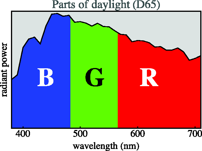
The Three Parts of Daylight Indicated in the Daylight Spectrum. The transitions between the parts are at 482.65 nm and 565.433 nm. An object that reflects all radiation in the blue part but nothing in the green and red parts will look blue, and so forth for green and red. The white object reflects all three parts completely. The best yellow paint will reflect the red and green parts, but not the blue. There are eight distinct such subsets; they define spectra whose colors are the vertices of the rgb cube. They are yellow, green, cyan, blue, magenta, red, white, and black.

blue part where $\chi (\lambda )=1$ for ${\lambda }_{\text{uv}}\le \lambda <{\lambda }_1$ , otherwise 0;

green part where $\chi (\lambda )=1$ for ${\lambda }_1\le \lambda <{\lambda }_2$ , otherwise 0;

red part where $\chi (\lambda )=1$ for ${\lambda }_2\le \lambda <{\lambda }_{\text{ir}}$ , otherwise 0,

where one may take ²² the approximate spectrum limits as ${\lambda }_{\text{uv}}=$ 380 nm and ${\lambda }_{\text{ir}}=$ 720 nm. The crate claims ca. 65% of the volume of the color solid (Figure 4; Bouma, 1946).

Figure 4.

The Skeleton Structure Induced by the Color Solid in cie d65 in the cie xy-Chromaticity Diagram (Left) and in cie xyz Space (Right). The red curve is the locus of $\chi (\lambda )=1$ for $\lambda >{\lambda }_2$ , ${\lambda }_2\in ({\lambda }_{\mathrm{uv}},{\lambda }_{\mathrm{ir}})$ , otherwise 0. The blue curve is the locus of $\chi (\lambda )=1$ for $\lambda <{\lambda }_1$ , ${\lambda }_1\in ({\lambda }_{\mathrm{uv}},{\lambda }_{\mathrm{ir}})$ , otherwise 0. The green curve is the locus of $\chi (\lambda )=1$ for ${\lambda }_1<\lambda <{\lambda }_2$ , $\overline{{\lambda }_{\mathrm{ir}}}<{\lambda }_{1,2}<\overline{{\lambda }_{\mathrm{uv}}}$ (the bar notation $\overline{\lambda }$ indicates the complementary wavelength of λ), otherwise 0. The purple curve is the locus of $\chi (\lambda )=0$ for ${\lambda }_1<\lambda <{\lambda }_2$ , $\overline{{\lambda }_{\mathrm{ir}}}<{\lambda }_{1,2}<\overline{{\lambda }_{\mathrm{uv}}}$ , otherwise 1. The crate has been indicated at right, its vertices colored for easy reference. At left, it appears as a triangle, as the chromaticity diagram is a projection from the origin. The triangle shows the gamut of chromaticities claimed by the crate. It is very similar to the gamut claimed by generic electronic display units. The curve marked with wavelengths is the spectrum locus, the horse shoe shape referred to earlier. We use this figure also to indicate that the cie xyz and rgb (remainder of the text) parameterizations can be used ex æquo in the representation of colorimetric structures. The rgb system yields more geometrically appealing and intuitive pictures though (e.g., Figure 5).

That these formally defined spectra indeed correspond to seen blue, green, red, and so forth is a remarkable fact of experimental phenomenology. It was noticed by Schopenhauer (1816) in an attempt to make scientific sense of Goethe’s (1810) intuitions. It is a brute fact because there can be no causal reason. Yet it cannot honestly be denied by generic observers.

Denoting the parts R, G, and B, any color (of some beam dominated by the standard) can be written as the color of rR + gG + bB, where $r,g,b\le 1$ . The beam rR + gG + bB will be referred to as the canonical representation of the color. The spectrum that gave rise to the color is metameric to the canonical representation.

The domain of the coefficients {r, g, b} is the unit cube ${\mathbb{I}}^3$ , which we will refer to as the “rgb cube.” The vertex {0, 0, 0} represents black (abbreviated k). The vertex {1, 1, 1} represents white (abbreviated w).

The remaining vertices may be divided into primary and secondary cardinal colors. The primary colors are {1, 0, 0} (r for red), {0, 1, 0} (g for green), and {0, 0, 1} (b for blue), whereas the secondary colors are {0, 1, 1} (c for cyan), {1, 0, 1} (m for magenta), and {1, 1, 0} (y for yellow). The cardinal colors occur in the natural periodic sequence ygcbmr. ²³ They are indeed “cardinal” because the only rgb cube points that lie on the boundary of the color solid. Proceeding from primary and secondary, we find that white is the unique tertiary cardinal color. Going in the reverse direction, we may add black. By construction, the pairs rc, gm, by, as well as kw are mutually supplementary (add to white). Standard colorimetry would reckon these “complementary with respect to the illuminant”; it has no natural notion of supplementarity.

All the vertices of the rgb cube lie on the surface of the color solid. The color solid (which is necessarily convex) appears as a slightly inflated unit cube (Figure 5).

Figure 5.

Three depictions of the color solid. At left, the rgb cube inside the color solid, depicted in rgb space. It is the largest (qua volume) inscribed crate to the color solid. Here, we split the color solid into two mutually congruent halves. The cut is by the red and blue curves shown in Figure 4 right. Notice that the color solid appears as a slightly inflated unit cube. This is also seen in the figure at right, which is a view from the outside. Notice that the vertices of the rgb cube lie on the boundary of the color solid.

On mapping databases of natural colors in color space, one finds that typically over 99% lie in the interior of the rgb cube. The ones that do not, have some coordinate only marginally different (0.01 range, see later) from 0 or 1. From a formal perspective, the rgb cube is the natural arena for the object colors (Küppers, 1978, 1989, 2005; Smith & Lyons, 1996).

Taking the conventional display color nonlinearity (often referred to as gamma correction; Poynton, 1993) ²⁴ into account, the rgb cube is very similar to the RGB pixel space of jpeg images (Pennebaker & Mitchell, 2004). Thus, one has a useful map from spectra to pixel values and even from pixel values to spectra (the canonical representations). The latter observation yields a very useful heuristic with numerous applications (see Figure 6). This renders the rgb representation much more convenient and intuitive than the conventional cie xyz representation (Figure 7).

Figure 6.

A Reflectance Spectrum of a Californian Poppy (Eschscholzia californica [Papaveraceæ]; Spectrum From the Floral Reflectance Database [FReD, reflectance.co.uk]) Flower and Its Canonical Spectrum. The poppy color under standard daylight is $\{0.156,0.057,0.016\}$ , the rgb coordinates are the levels of the canonical representation.

Figure 7.

The Color Matching Functions. At left, the cie xyz color matching functions; at right, the rgb color matching functions that refer to the parts of daylight (Figure 3) as primaries. They are simply linear combinations of each other; thus, they lead to exactly the same colorimetry. (Colors used in the graphics at left arbitrarily chosen.) The rgb representation is far more intuitive in applications to the life sciences, as it allows much clearer graphical representations in virtually all cases. (In this case, the colors used in the graphics at right signify the “red” [long wavelengths], “green” [medium wavelengths], and “blue” [short wavelengths] parts of the partition of white.)

The construction of rgb space is based on average daylight. That is exactly why the representation is intuitive and useful in biological contexts. Without a designated illuminant, there is not much formal structure. However, because daylight may vary capriciously, one should be prepared to handle such variations (see later).

Colorimetry of Object Colors

Again, the standard setup, that is the simplest possible setting, considers colored papers, laid out flat on a tabletop and illuminated by a uniform source, such as the northern sky, the classical illumination of artist’s studios (Friel, 2010).

Let the object gamut contain a white object. It serves to anchor the gamut (Gilchrist et al., 1999). This is a bare bones context from which one may deviate, or articulate into various directions.

Let the radiance of the beam scattered by the white reference be denoted $D(\lambda )$ . Let spectral reflectance factors be denoted $F_i(\lambda )$ (the index i ranging over the various objects). Then, the beam scattered to the eye by the $i\text{th}$ object is $F_i(\lambda )D(\lambda )$ . One finds the parameters $\{r_i,g_i,b_i\}$ such that $r_{i}R+g_{i}B+b_{i}B$ and $F_i(\lambda )D(\lambda )$ are metameric. This involves the color matching functions shown in Figure 7 (right). ²⁵ One also finds the parameters $\{r_0,g_0,b_0\}$ such that $r_{0}R+g_{0}B+b_{0}B$ and $D(\lambda )$ are metameric. Then, one defines $\{r,g,b\}=\{\frac{r_i}{r_0},\frac{g_i}{g_0},\frac{b_i}{b_0}\}$ as the colorimetric coordinates of the object color defined by the reflectance F_i. The division implements “color constancy” (Olkkonen et al., 2009; von Kries, 1905).

This forces the object colors to lie in the unit cube ${\mathbb{I}}^3$ , henceforth referred to as the rgb cube. ²⁶ The division by the white reference implements an adaptation, or anchoring, that is familiar from phenomenology (Gilchrist et al., 1999).

The white object serves to scale for the overall radiance. That is to say the illuminant $D\prime =\alpha D$ with $\alpha >0$ will yield results that do not depend on α. Thus, we have modeled the “adaptation” that is well known to apply to a huge range of radiances in the case of human vision.

An extrapolation of this is to admit spectral variations and uses illuminants $\overline{D}(\lambda )$ instead of $D(\lambda )$ , while using the same formalism throughout. For the white object, this has the effect that it is invariant against spectral changes of the illuminant. It is trivially true for the black object too and thus for the kw body diagonal of the cube. It is not necessarily true for the other colors.

How useful this is, is a matter of empirical investigation. The intuition is that it should work fine for relatively minor variation about the standard illuminant. This implements the automatic white balance of human vision. The mechanism is similar to the “von Kries coefficients Law” ²⁷ (von Kries, 1905).

When the spectrum of the illuminant is changed, the color solid itself changes, and the inscribed crate can no longer be the largest one. It will remain very close to that for relatively minor spectral variations, though. Colors might conceivably move in or out of the rgb cube. In the (ecologically valid) settings considered here, this is exceedingly rare (see later).

How descriptive this model is can only be judged on the basis of variations that remain in the ecologically valid range. Thus, the issue has to be investigated on the basis of statistical models of the generic environment (Koenderink, 2018b).

There can hardly be any doubt that visual systems evolve according to Umwelt (both ecology and anatomical/physiological apparatus) and Lebenswelt (or lifestyle) ²⁸ (see von Uexküll, 1926, 2010).

Ecological Variations

Colorimetry as such has nothing to say about the structure of color space, except that it is a linear space. Color space is just a projection of the space of spectra.

There are two, categorically distinct, ways to explore the metrical structure of color space. One is psychophysics. For instance, one might measure hue discrimination (Farnsworth, 1943; van Esch et al., 1984; Wright & Pitt, 1934), or even general just noticeable differences all over color space (MacAdam, 1942, 1947; Noorlander & Koenderink, 1983). It defines a graininess and a Riemann metric. One finds that human observers may differentiate as many as 10 ⁶ to 10 ⁷ colors (Wyszecki & Stiles, 1967). This suggests an uncertainty of about 0.01 in the rgb coordinate values (Koenderink et al., 2018). ²⁹ This is not unreasonable in view of the thumb rule of 1% for the Weber fraction of radiant powers.

Other ways to explore structure is through phenomenology (for instance, Munsell, 1905, 1912) or through ecology (Koenderink, 2018b). The latter is the main topic of this section. The biological perspective suggests that the phenomenological resolution will have evolved to match the uncertainties due to ecologically valid variations.

The Realm of Illuminants

For diurnal, terrestrial animals, the illuminants are varieties of daylight. Daylight changes with time of day, meteorological conditions, and ambient scattering (Koschmieder, 1925; Schuster, 1905; Strutt, 1899).

Exceptions that we ignore are such radiant sources as the bioluminescence of glowworms, fire light, and so forth. Glowworm light is a vital issue in the glowworm world, even if it is a mere curiosity in ours. Different animals, different realities. Hominins are no less special cases than the Lampyridæ are. In biology (psychology is different by design), anthropocentrism implies dubious science.

There are two aspects to this: the Umwelt and the lifestyle. The Umwelt contains all the ways the environment can work on the animal. For humans, this includes radiation in the visual band but excludes radio waves. It also includes all the ways the animal can work on the world. For humans, this includes moving stones but excludes generating strong electric fields without assisting technology.

Animals may live in very different Umwelts. The lifestyle involves the use of Umwelt elements in the course of generic actions (von Uexküll, 2010). For instance, the tiger and the lamb have similar Umwelts but very different lifestyles.

The ecologically valid realm of illuminants is evidently the range of daylight spectra. Hominins might have known fire light as a case of secondary importance. Yet it is the daylight—hunting–gathering time—that would have driven their evolution.

Fortunately, there exist databases that cover daylights under parametric variation of:

time of day	dusk to dawn
meteorological circumstances	open weather, overcast, fog, hydrometeors
geographical latitude	the height of sun at noon
season	the height of sun at noon, atmospheric haze
ambient scattering	scattering from vegetation, bushes, trees

and a few more. Because it is awkward to mix databases, we use just a single database from the Kohonen laboratory (Kohonen et al., 2006; examples in Figure 8). It should cover most ecological variation. This database contains 52 radiant spectra.

Figure 8.

Some Instances Taken From the Kohonen Daylights Database (Kohonen et al., 2006).

This database may well be slanted toward extreme cases. Anyway, the major influence of the illuminant is by way of spectral slope (color temperature) and (already much less so) spectral curvature. The more or less random component due to environmental factors (Morimoto et al., 2019) hardly plays a quantitatively important role.

The Realm of Objects

The primordial object for the terrestrial, diurnal animal is a volumetric region (its interior not optically revealed) bounded by an opaque, approximately Lambertian scattering surface. Think of a potato. Local surface elements of such objects scatter the same radiant beam to the eye from wherever the animal might be with respect to the object. The large majority of biologically important objects in nature are of this generic type. These include stones, earth, vegetation, animals, and processed things such as roots, wood, bones, meat, fat, and more. Even huge areas in the visual field such as the sky or large expanses of water fall in a different class. Their colors tend to be of little interest when you are hunting, or gathering, for your daily meal.

Common exceptions from our contemporary Umwelt tend to be man-made; think of polished metals. They came into existence after the evolution of hominin vision was already well on the way to its current state. A mirror has no color. The beam scattered to your eye depends critically on your position. In a hall of mirrors you are lost, albeit differently from being lost in the woods. In a hall of mirrors you may run into the walls, but in a forest, there is no reason to run into tree trunks. Tree trunks are bona fide visual objects, whereas mirrors are not.

It is difficult—indeed, probably impossible—to define an ecologically valid, statistically balanced, generic range of objects. It should certainly include:

vegetation	leaves, flowers, bark, moss, grass
internal or subterranean parts	fruits, nuts, roots
animal coverings	skin, fur, scales, feathers
animal internal parts	flesh, fat, bones, gut
minerals	earth, stones, mineral pigments

A study of spectral reflectance factors suggests that the spectral articulations found in these classes are statistically very similar.

For a start, we select two databases: one on vegetation (Kohonen et al., 2006; examples in Figure 9) and one on mineral pigments.^30,31 The vegetation database has 219 items: leaves, stems, flowers, and dry brown leaves. The mineral pigments database has 723 items of mainly classical painter’s pigments in powdered, dry form. After deleting samples with a significant specular component, 651 items are left. We let these represent the “earth colors” as different from the vegetation colors. Perhaps unfortunately, we are missing animal colors. There appears to be no suitable databases in the public domain. A spot check on spectral reflectances of bone, fat, meat, and skin suggests that it would hardly change the picture much, if at all. We feel that we cover the realm sufficiently.

Figure 9.

Some Samples From the Finnish Vegetation Database (Kohonen et al., 2006).

Perhaps regrettably, we have no data on the frequency of occurrence or on the relative relevancy for the hunter-gatherer lifestyle. Our choice is likely to overrepresent singular outliers. But perhaps this is not such a great disadvantage. We are likely to obtain a somewhat pessimistic view of the ecological graininess.

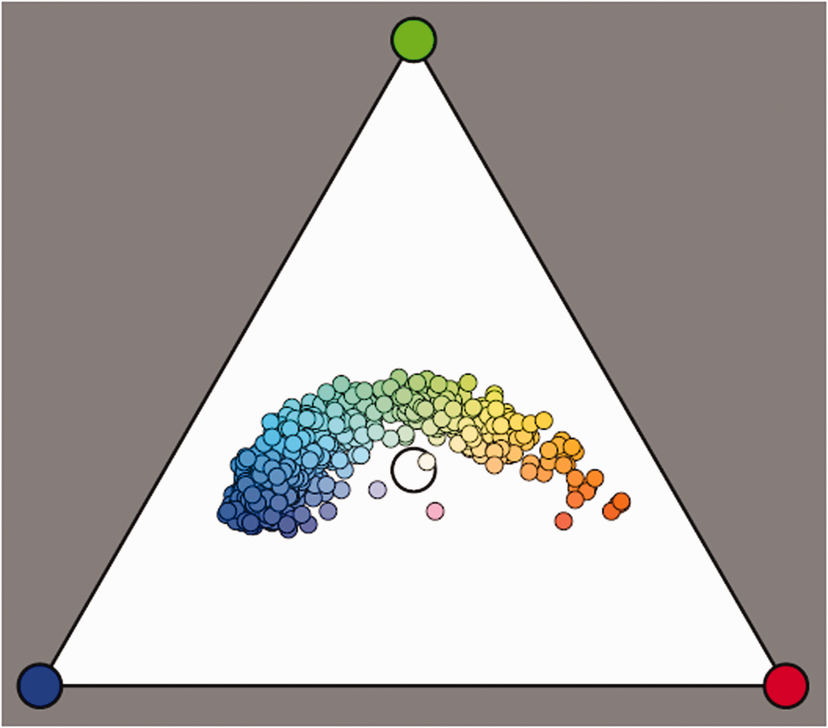
Neither database fills the rgb cube more or less homogeneously (Figure 10). This is indeed typical of all ecologically valid databases. The convex hull of the colors in the vegetation database claims 21% of the volume of the cube and that of the mineral pigments claims 44%. Because convex hull volume is essentially determined by the outliers, these are certainly overestimations.

Figure 10.

The Distributions of the Vegetation Database (Left) and the Mineral Pigments Database (Right). These are the colors under the standard source cie d65.

Figure 10 yields a good illustration of our earlier remark that in practice almost all object colors lie in the interior of the rgb cube. For the vegetation database, there are three cases (out of 219) in which the green coordinate is less than $-0,01$ , the actual values being –0.0186, –0.0171, and –0.0118; there are no values greater than 1.01. For the mineral pigments (among more containing the most vivid artist’s pigments), there are 5 cases in the red, 35 in the green, and 3 in the blue with coordinate values less than 0, and there are 2 cases in the red for which the coordinate values exceeded 1. In the former case, the median undershoot is 0.018, and in the latter, the overshoot is 1.026. This is typical; it is one reason why the rgb representation is so useful. ³²

The Graininess Induced by Illumination Changes

A very straightforward investigation simply puts all objects under all illuminants. Thus, we obtain 52 colors for each object. To streamline the presentation, we summarize these sets by covariance ellipsoids at the 95% level (Figure 11).

Figure 11.

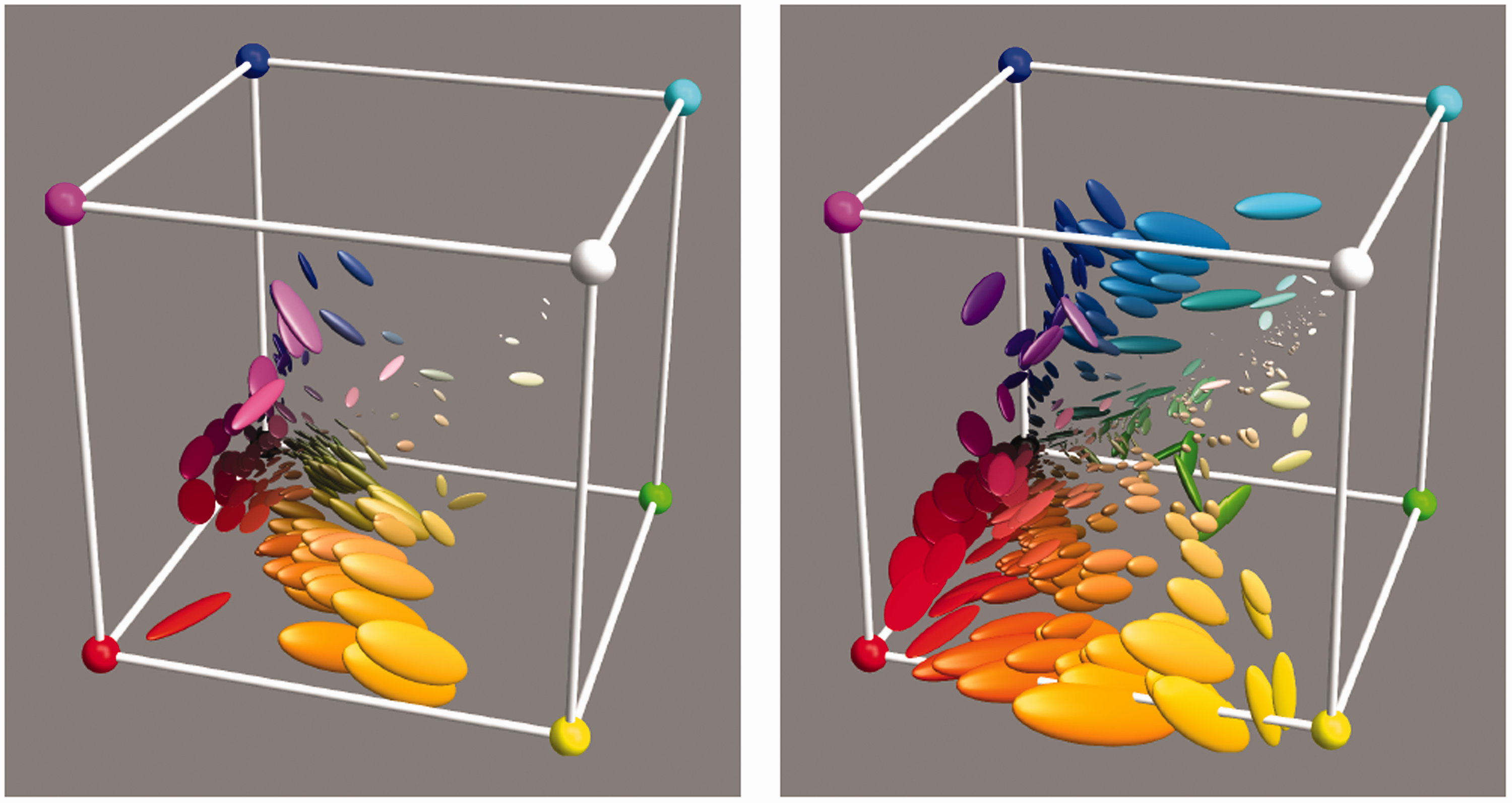
The 95% Confusion Ellipsoids Due To the Variation of the Illuminant for the Items in the Vegetation Database (Left) and the Mineral Pigments Database (Right).

We find that the automatic white balance works really well. This perhaps reminds one of results obtained by hyperspectral imaging (Nascimento et al., 2002). Although the illuminants vary over the full daylights database, the various items stick quite close to the location they have when illuminated by the standard source (Figure 10).

The capricious variations of color appearances, noticeable as deviations from color constancy, cannot be accounted for by the observer on the basis of available visual observations. They are due to hidden variables and thus naturally occur magically.

We define the equivalent radius of an ellipsoid as the radius of the sphere with the same volume as that ellipsoid. We also define the maximum radius as the maximum semiaxis of the ellipsoid.

For the vegetation database, the range for the equivalent radius is $(0.000,0.059)$ , and the quartiles are $(0.006,0.013,0.02)$ . The range for the maximum radius is $(0.000,0.165)$ , and the quartiles are $(0.019,0.034,0.058)$ .

These numbers are in terms of the edge length of the rgb cube; thus, they are quite small. The mean ellipsoid volume is only $5.4{10}^{-5}$ of the volume of the rgb cube. This implies a Weber fraction per rgb coordinate of a few percent (take the cube root); thus, it exceeds the psychophysical discrimination level. It provides for about 20,000 (take the reciprocal) distinct colors, much higher than numbers from experimental phenomenology (about a thousand).

For the mineral pigments database, the range for the equivalent radius is $(0.000,0.076)$ , and the quartiles are $(0.002,0.008,0.019)$ . The range for the maximum radius is $(0.000,0.0076)$ , and the quartiles are $(0.006,0.024,0.053)$ . Thus, there is not much difference in the results for the two, ontologically very different, databases.

The confusion ellipsoids are evidently not isotropic. There is apparently an overall trend, although there is hardly a smooth field on the local scale. One reason for a trend is probably the fact that the daylight spectra differ mainly in one, at most two dimensions (the spectral slope and curvature, the slope being the dominant factor). The more or less abrupt variations are expected. They are doubtless due to the idiosyncrasies of the object spectra. These differ from the corresponding canonical spectra in manifold ways. One expects that taking the metamers of the object spectra into account would tend to smooth things out.

The Additional Graininess Induced by Metamerism

Both conceptually and technically, metamerism poses a problem. It is quite clear what has to be done in principle though, namely:

Given a color, determine the ecologically valid set of (mutually metameric) spectra that will yield this color under the standard illuminant;

Determine the color of each of the metamers as seen under all ecologically valid illuminants;

Summarize the resulting distribution, for instance, as a covariance ellipsoid;

Repeat this for all colors in the rgb cube.

Problems are that the color is not likely to be in the database and that the database will not yield a set of representative metameric instances. For investigations of this type, the existing databases are hugely insufficient. The only way out is to summarize the databases in terms of generative statistical models (Griffin, 2019; Koenderink, 2010b; Koenderink & van Doorn, 2017; Zhang et al., 2016).

Of course, setting up such statistical models is a worthwhile scientific enterprise by itself. It has to be one of the fundaments required in studies of the evolution of the human visual system.

To be able to proceed, we first need to consider some basic complications one immediately runs into in an attempt to implement this program. These mainly involve methods to deal with the nature of the domains. Such methods should not rely solely on formal methods. They need to be rooted in concepts from basic physics.

Dealing With the Nonlinear Constraints

The computational machinery of formal colorimetry is linear algebra. This cheerfully operates with entities that have no possible physical existence. Such entities (such as the elements from the null-space of the color matching matrix) may well represent very useful virtual objects. However, eventually both the input and the output of computations need to represent physical entities.

Physics introduces a number of constraints on the objects that formal colorimetry works with. In a more positive vein, the physical constraints yield very important structures. The color solid itself is a prime example of that.

Failure to reckon with physical constraints easily leads to erroneous results. A common instance involves nonphysical predictions being “cured” by clipping. Principal components analysis (PCA) is often made to work that way.

It should be recognized when something is fundamentally flawed. Correct methods should make it impossible to ever obtain nonsensical results. In most cases, the solution is to use some variety of homomorphic filtering (Oppenheim et al., 1968).

The Nonnegativity of Radiant Power

Radiant power is necessarily nonnegative. An obvious way to deal with this is to consider the logarithm of radiant power (Koenderink & van Doorn, 2017). This is very natural from the perspective of physics. Most interactions involving radiant power are of a multiplicative nature. Another reason is that the fully noninformative Bayesian prior is hyperbolic, therefore uniform on the log scale (Jaynes, 1968, 1973). The general method to deal with the constraint is to use a variety of homomorphic filtering. One maps the radiant power to the logarithmic (one might call it the physical) domain, operates on it (e.g., does various statistics), and transforms back.

In the physical domain, one may use linear methods, as the structure of ${ℝ}^{+}$ was transformed into $\mathbb{A}$ , the full affine line. This solves any sign problems with PCA. Another problem with PCA is that it requires a metric. In using PCA, a default metric tends to be silently (or even upfront; Lenz, 2002) assumed. It really should be a first consideration. It requires reasons based on considerations of physics. Here, the logarithmic transform also helps out, because the Bayesian prior becomes uniform.

Dealing With the Finite (0,1)–Reflectance Range

The domain $\mathbb{I}$ , the unit interval, also renders the use of linear methods, such as PCA, fundamentally flawed. Nevertheless, it is often used (Chiao et al., 2000; Lenz, 2002; Maloney, 1986). Only sheer luck prevents sign, or overflow problems to emerge. The conventional solution to simply clip results to the unit interval is a mere kludge.

The reflectance is ultimately due to optical processes that depend on physical parameters such as absorption and scattering cross sections. Such physical quantities are defined on the nonnegative reals, suggesting that one should identify the appropriate physical domain. This is complicated, because various processes may account for ecologically relevant reflectance factors.

Perhaps the dominant process is well described in terms of the Kubelka–Munk theory (Joshi et al., 2001; Kubelka, 1948, 1954; Kubelka & Munk, 1931) of radiative transfer in layered, turbid media. This applies to papers, paints, and textiles in our present society (Hubbe et al., 2008; Judd & Wyszecki, 1975; Pauler, 2001; Stenius, 1951a, 1951b, 1953; Van den Akker, 1949). Perhaps more appropriately, it equally applies to earth, vegetation, skin, and bones in the hunter-gatherer’s world.

The reflectance depends upon the ratio of the absorption K and scattering S cross sections. This spectral signature K/S is widely used in materials research. It only depends on physical quantities that live in ${ℝ}^{+}$ . This suggest that the appropriate physical domain is the logarithm of the spectral signature, that is $\log (K/S)$ .

The spectral signature depends only upon the scattering and absorption cross sections and thus is a true object property. Using the Kubelka–Munk theory, one can move back and forth between the spectral reflectance and the spectral signature. To do that, we define a pair of mutually inverse functions $f(r))$ and $g(\rho )$ (Appendix A, Figure 12).

Figure 12.

The Function f(r) (Left) and $g(\rho )$ (Right). Notice that $f:\mathbb{I}\mapsto ℝ$ , whereas $g:ℝ\mapsto \mathbb{I}$ .

The spectral signature is simply related to the reflectance factor of an optically thick turbid layer. The function $f(r))$ maps the unit interval $\mathbb{I}$ on the full affine line $\mathbb{A}$ , and the inverse function $g(\rho )$ maps the full line to the interval (Figure 12).

That this is generally a good idea is clear when one compares histograms of pixel values in photographs of vegetation (tundra or savannah-like scenes). Although the raw pixel histograms tend to be complicated, often bimodal, the histograms in the physical domain tend to look much more unimodal and symmetric (Koenderink & van Doorn, 2017). It is apparently the more appropriate domain for statistics. This is another instance of homomorphic filtering. In any case, one tries to map from the ecological to some appropriate physical domain.

One may meet with a variety of physical processes. In any specific case, one identifies the most appropriate homomorphic representation. This calls for a broad familiarity with classical physics (Feynman et al.,1964–1966).

Statistical Models of the Illuminant

For the purpose of colorimetry in the context of the hominin Umwelt, the absolute levels of radiant power are largely irrelevant. It is mainly the spectral distributions that count. So the first thing to do is to somehow normalize the individual items, perhaps by shifting them in the physical domain.

All instances are eventually due to sunlight, filtered by the atmosphere and affected by ambient scattered radiation. These are all multiplicative processes that become additive in the physical domain.

Sunlight derives from the sun’s photosphere and is essentially thermal radiation of a ${5777}^{°}\text{K}$ black body, articulated by a number of atomic absorption lines. Filtering by the atmosphere introduces additional molecular absorption, as well as the effect of extinction due to Rayleigh scattering and perhaps ærosol scattering. This basic structure will reappear in all instances. Thus, the ensemble mean in the physical domain is meaningful.

Time of day and height above the horizon are expected to lead to changes of overall slope and perhaps curvature. These are most properly caught by the low-order PCs. Remaining variations are likely to be due to a variety of random causes. These are most appropriately modeled by some fractal signal. There is perhaps something to say for using Planck’s formula for thermal radiation augmented by a low-order polynomial model for the deterministic part. For many applications, that would avoid overfitting. In our application, the microarticulation had perhaps better be retained. They might accidentally correlate with microarticulations in spectral reflectance factors.

The main decision is the level at which the deterministic (PCA) low order should give way to some random fractal. It appears to be the level after the PCs that essentially represent curvature or perhaps cubical structure. This yields a simple model that may serve to generate novel instances of “daylight spectra” (Figure 13).^33,34 We use the ensemble mean, a linear combination of the PCs with coefficients generated by a multinormal distribution (using the distribution of projections of the database instances on the PC-basis to define the covariance matrix), and a fractal fuzz. Finally, we transform to the ecological domain.

Figure 13.

Chromaticities of a Number of Random Daylight Instances. This convenient (because symmetrical in r, g, b) chromaticity diagram is the projection from the black point on the triangle spanned by the red, green, and blue vertices of the rgb cube. It was used by Maxwell and by Helmholtz as a natural representation. The cie has pushed the deformed version (cie xy chromaticity diagram) that includes properties that not belong to colorimetry per se (luminance) and that can be found all over the Internet.

The nature of the “fractal fuzz” is estimated from the slope of the power spectrum of the residual structure, after subtracting the PCA approximation.

Statistical Models of the Objects

In this case, the absolute level is important. Thus, we do not normalize in any sense. We just move to the physical domain, assuming radiative transport in turbid layers as the dominant process. There is no a priori reason to expect a bias in spectral slope or curvature. One expects the spectral articulation to be translation invariant in a statistical sense. The reason is that the visual range is very narrow and does not involve switchovers between distinct physical processes. Molecular mechanics dominates the infrared, atomic electronic transitions the ultraviolet, whereas the visual range largely involves various changes in chemical constitution induced by the impinging photons (Feynman et al., 1964–1966). This is also the reason why this range is of major biological significance.

To have a rough check, we compute the histograms of spectral radiant power density over the whole vegetation database as a function of wavelength (Figure 14, left). One finds some structure that might well prove specific for the vegetation database. We also find an overall slope (see also Griffin, 2019) that might well have a generic relevance.

Figure 14.

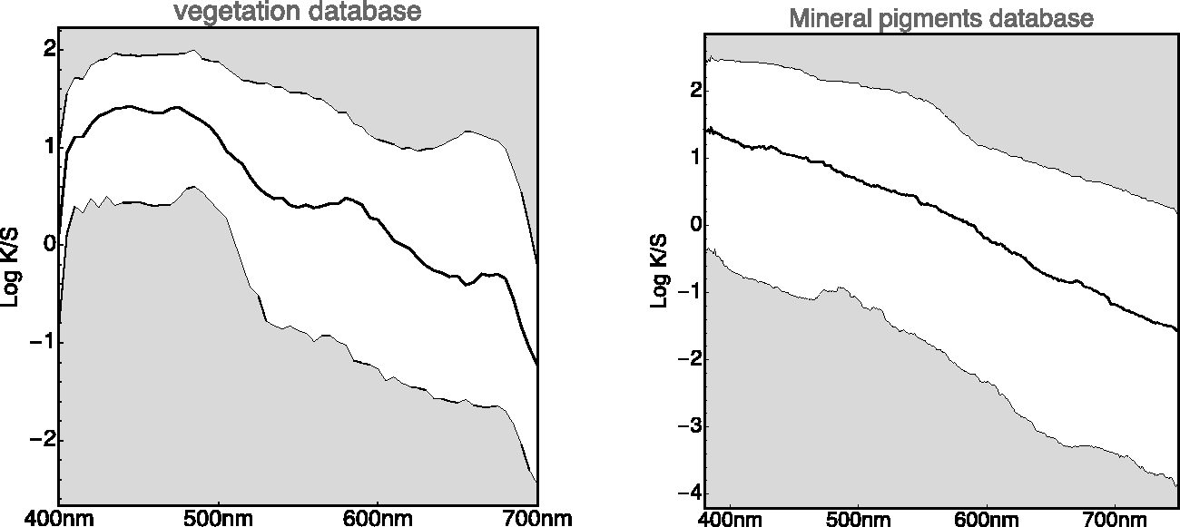
Summarized “Spectral Histograms” of the Vegetation Database (Left) and the Mineral Pigments Database (Right). “Summarizing” implies plotting the median and quartile ranges as a function of wavelength. In addition (not shown here), one tests for approximate normality of the distribution as a function of wavelength. (Note. The logarithm used here is the natural logarithm, different from Figure 15. Whenever the base 10 logarithm is used, we use the notation ${ }^{10}$ Log.)

At first blush, it perhaps looks like an imprint of the chlorophyll absorption spectrum. One way to check this is a comparison with databases of very different materials, say minerals (Figure 14, right). Here, we find the same slope, so the chlorophyll bands, typical for vegetation, are apparently not the issue. It rather is something generic that should at one point receive an explanation in terms of ecological physics. The items from the minerals database have a higher resolution (380–780 nm at 1 nm intervals); moreover. the database volume is larger than that of the vegetation data. As a result, the spectral histogram is less noisy. One notices a well-defined spectral gradient of the spectral signature with wavelength. Notice the similar trends in these very different databases. We have not seen such summaries as in Figure 14 elsewhere (but see Griffin, 2019). They evidently are a must-have in all cases.

The average wavelength dependence probably derives from the size of the microparticles in the granular media, as chemical properties are apparently irrelevant. Particle sizes are in the ten to a hundred micrometers range; thus, neither Rayleigh nor Mie scattering theories apply. The type of analysis that might apply is discussed in Pilorget et al. (2016).

The behavior near the uv spectrum limit seen in Figure 14 may be due to instrumental problems. It is absent in a huge database obtained from hyperspectral imaging, ³⁵ which otherwise reveals the same pattern. We have only used the latter database to check whether trends are similar to the databases used here (they are). The reason we do not use this huge hyperspectral database further is that this database seems very uneven and is likely to be troubled by systematic errors pertaining to large subsets of items.

Because the flower spectra look rather diverse, a generic model might simply be a random fractal. We find the Fourier power spectrum of the spectral articulation (of course, in the physical domain; see Figure 15). It turns out to fall off as the inverse fourth power of frequency in all databases we tested. Thus, a fractal dimension of two seems indicated. This suggests a simple model of the phenomenological optics (see also Griffin, 2019).

Figure 15.

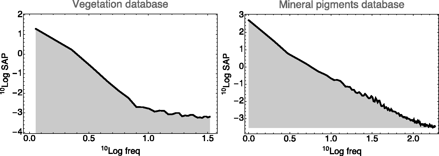
The Power Spectrum of the Spectral Articulations of the Vegetation Database (Left) and the Mineral Pigments Database (Right). The frequency is in cycles per visual range. (We let sap stand for “spectral articulation power.”) Signals were carefully windowed and so forth. The two databases are available on slightly different spectral ranges. One notices a fall off by an inverse fourth power. Such spectra are another must-have for any database.

The spectrum will be the result of various (perhaps many) mutually independent physical causes. Each process will imprint a local structure on the spectrum at some random location. For the present purposes, the spectral width of the local structures is the relevant property. For a start, one considers just a single width and a random, uniformly distributed location. A simple, generic model of this physics is provided in Appendix B (see Koenderink, 2010b; Koenderink & van Doorn, 2017).

The model allows a formal description of the autocorrelation function of the spectral articulation. The formalism relates it to the power spectrum. From the empirical power spectrum, we estimate that the halfwidth of the autocorrelation function is about the width of the visual range (Koenderink & van Doorn, 2017). This implies that natural spectra are not highly articulated. They vary only gradually with wavelength.

This suggests a very simple algorithm to generate instances.^36,37 One generates a fractal and adjusts its variance to that encountered in the database. One adds either the database mean, or just a constant slope. Converting from the physical to the ecological domain then yields the instance. As seen in Figure 16, such instances fail to fill the rgb cube. This is only natural (Koenderink, 2010b) but is also inconvenient (see later).

Figure 16.

The Colors of a Number of Instances From the Reflectance Algorithm Fail to Fill the rgb Cube (Left, Samples; Right, Their Chromaticities [see Figure 13 legend] and the corresponding convex hull). This is expected (compare Figure 10).

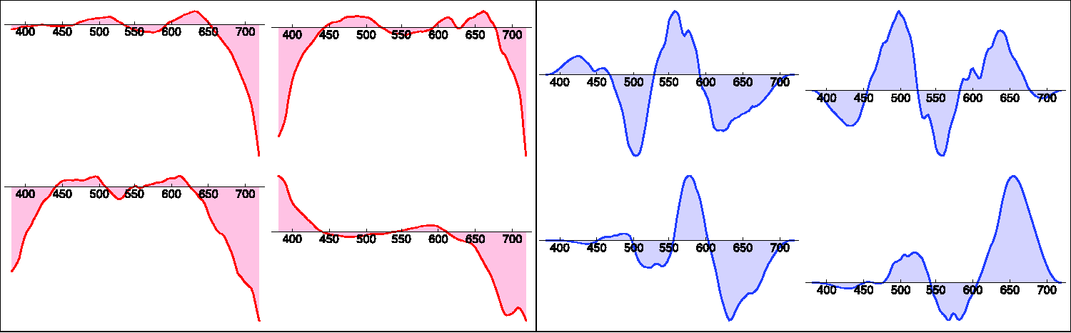
In Figure 17, we show examples (for clarity only 16 × 16 = 256 samples each) of instance of daylight and object colors generated by the statistical models.

Figure 17.

Instances of Daylight Colors (Left) and Object Colors (Right) Generated by the Statistical Models. The daylight colors have been normalized to have the maximum rgb coordinate value 1; the object colors are shown under the standard cie d65 illuminant. The models proper generate spectra, of course, not colors.

Generating Metamers

For this investigation, we need to be able to generate arbitrarily many metamers for any given color. This is substantially complicated by the constraint that the metamers should be ecologically valid. Generically, there exist infinitely many mutually metameric spectral reflectance factors that will generate the given color under the standard illuminant. However, the overwhelming majority fails to be acceptable as an ecological valid reflectance. Thus, one needs to design specific methods for this case.

The databases let one generate ecologically valid metamers as linear combinations of random instances. Given three of such instances, one may combine them to yield the given color. The result will be reasonable if the three instances have colors close to that of the given color. Here starts a problem; for the databases, let one find colors only in a part of the rgb cube. Moreover, the databases yield not sufficient variation in the neighborhood of any item.

One (partial) solution is to limit the investigation to colors within the convex hull of the database colors. From a pragmatic perspective, this is not even such a bad idea. Colors far outside the convex hull are likely to be irrelevant anyway.

For more formal investigations, a way out of this problem is to generate metamers as metameric variations of canonical spectra. Because there always exists a canonical instance, this is guaranteed to work for all colors. All one needs to do to generate metameric variations is to add random metameric blacks to canonical spectra. Of course, such metameric blacks should themselves be ecologically valid.

One easily generates such metameric blacks by generating four random instances and combining them linearly so as to obtain a black color modulo the amplitude. ³⁸ Unfortunately, this tends to lead to unreasonably large amplitudes near the spectrum limits (Figure 18). ³⁹ It renders the metameric blacks ineffective due to the physical constraints. Because the reflectance should be in (0, 1), the maximum amplitude of a perturbation is limited by that (Figure 19). A simple cure is to use a Hanning window ⁴⁰ over each of the four instances. This leads to metameric black spectra that have appreciable amplitude in the region that counts and are statistically much closer to the databases (Figures 18 and 19).

Figure 18.

Four Random Black Reflectances Without (Left) and Four With (Right) the Use of a Hanning Window. In practice, such apodization is necessary.

Figure 19.

These Are Metameric Spectral Reflectance Factors for the Average Gray Color $\{0.5,0.5,0.5\}$ . The black reflectances have been maximally scaled, that is, till the reflectance values hit one of the zero or one constraints. These are obviously quite “bad” grays, although they—by design—appear perfectly identical under the standard illuminant.

We construct random metameric reflectance spectra for a given color by adding ecologically valid black spectra to the canonical spectrum. This allows us to reach any point in the rgb cube. Unfortunately, this does not take account of the probability density of metameric blacks. This no doubt depends upon the location in the rgb cube.

It is a priori clear that colors on the boundary of the color solid are unique, that is, have no metamers. This is because the corresponding spectra have values of either 0 or 1, thus cannot be freely perturbed. For our choice of canonical spectra, this also applies to the boundary of the rgb cube.

The probability density of the metameric black amplitudes is something we do not have access to. We simply use the maximum values; thus, our estimates of the influence of metamerism are certainly overly pessimistic. The examples (Figure 19) of metameric grays reflect that.

The Overall Graininess Due To Ecological Variation and Constraint

In an extensive investigation, we start with any color coordinates, call it the fiducial color. We find its canonical reflectance and perturb it with a random black. Next, we find a random instance of a daylight spectrum. Then, we compute the color and the color of the white reference, and from these, the new color coordinates. These latter will typically differ from the color coordinates we started with. We repeat this a hundred or a thousand times (say) and determine the covariance ellipsoid of the resulting set of colors that surround the fiducial one. ⁴¹ In Figure 20, we show an example, a thousand instances at the center of the rgb cube, $\{0.5,0.5,0.5\}$ .

Figure 20.

A Thousand Samples at Median Gray (Red Points). The bluish ellipsoid is the 95% boundary. This yields a good notion of the nature of the summary description by way of ellipsoidal volumes (bluish volume).

Repeating this procedure for many colors, we obtain a sampling of the field of covariance ellipsoids over color space (Figure 21). This defines the grain due to metamerism for the given ecological constraints. As expected, the confusion regions are larger than in the case of mere illuminance variation (Figure 11). This is due to the inclusion of metameric reflectances. The range of the maximum radius is $(0.038,0.220)$ , and the quartiles are 0.087, 0.119, and 0.145. The range of the equivalent radius is $(0.012,0.079)$ , and the quartiles are 0.033, 0.041, and 0.051.

Figure 21.

The 95% Confusion Ellipsoids in rgb Display Space ( $\gamma =2.2$ ). This yields a realistic view on the size of the ellipsoids in jpeg photographs with automatic white balance. At left, a view that shows the black–white and green–magenta dimensions to best advantage; at center, a view that shows the black–white and red–blue dimensions to best advantage; and at right, a view that clearly shows the distribution over hues.

The mean ellipsoid volume is $4.17{10}^{-4}$ ; thus, one estimates that there is ample room for over a thousand distinguishing marks. Thus, the proof (see Appendix C) that colors are not fit as object properties (in general!) is robbed of much of its grim impact. The proof simply does not apply to niches, like the human hunter-gatherer tundra or savannah existence. In retrospect, this was to be expected. The present calculations pin it down quantitatively.

The mean ellipsoid volume of $4.17{10}^{-4}$ suggests a Weber fraction per rgb coordinate of about 7% to 8%. This far exceeds the psychophysical discrimination thresholds but is comparable to estimates of color reproduction from experimental phenomenology (Koenderink et al., 2016, 2018). These estimates are roughly comparable with estimates based on hyperspectral images of natural scenes (Linhares et al., 2008; Marin-Franch & Foster, 2010).

Discussion

The Graininess of Human Color Vision

Psychophysical grain size data show that humans may resolve in the order of 10 ⁶ to 10 ⁷ colors (Pointer & Attridge, 1998). Such psychophysical data are based on just noticeable differences (jnds) that consider only the segmentation function. They disregard the function of color as label, or as distinguishing mark. The jnds are likely due to physical (photon noise) and physiological factors. A number like 10 ⁶ is at least three orders of magnitude larger than the grain size suggested from our investigation of the ecology.

In a recent investigation (Koenderink et al., 2018), we had 50 observers synthesize a total of 3,000 randomly selected colors using a color picker (Koenderink et al., 2016). The task made it impossible to rely on a common boundary, or transition region. The observers had to look back and forth between the fiducial and the target that they had to adjust. It was also impossible to compare either fiducial or target to a common background. In such a setting, the errors become very much larger. We found that humans resolve about 10 ³ rgb colors if they are forced to use colors as distinguishing marks. Physical or physiological factors cannot be responsible for this grain size. These data address the factors of biological relevance (Gegenfurtner & Rieger, 2000; Koenderink, 2018b; Olkkonen et al., 2009) as opposed to physical limits.

The precise distribution of the covariance ellipsoids found in our study (Koenderink et al., 2018) is not clearly reflected in the calculations (Figure 21). This is perhaps to be expected, as the calculations take no account of ecological or ethological weights. However, the overall magnitudes are in the right ballpark. The difference of three to four decades in size between these ellipsoids and the jnd volumes may appear huge. However, taking trichromacy into account, it drops to a factor of perhaps a little over 10 (take the cube root). This renders the number intuitively acceptable.

The grain induced by ecological variations limits the number of colors that might be used as distinguishing marks under all circumstances to about 10 ³ . This seems amply sufficient for most hunter-gatherer needs. Colors as distinguishing marks are really useful in the ecological setting, although they are formally proven useless in general.

Colors as Object Properties

Are colors object properties? Our findings immediately relate to this question. It addresses an issue that has been widely debated in philosophy (Byrne & Hilbert, 2003). From a general and logical perspective, the answer has to be in the negative. Our formal, constructive proof in the Appendix leaves no doubt. It degrades colors to mere mental paint. Neither are Roses Red, nor are Violets Blue.

However, colors remain useful labels of things from the ecological perspective. Thus, the biological answer to the question has to be in the affirmative. For all practical purposes, colors are object properties. This conviction is reflected in the significance conventionally attributed to the colors of national flags. Roses are Red, Violets are Blue. The question of whether colors are object properties is an academic one. “Object properties” or not, colors are certainly useful as distinguishing marks. They boost biological fitness.

This will be hardly surprising from most people’s intuition. Color is obviously one distinguishing mark that helps deciding between tomatoes and lemons. Perhaps oddly, a scientific backing of this intuition is lacking thus far. Our study solves this issue from a pragmatic, biological point of view—at the same time putting the intuitions of philosophers in the right. Colors are useful distinguishing marks for a hunter-gather existence in tundra or savannah ecologies.

Note that this does in no way imply that colors may not have other biologically important uses. For instance, they are instrumental in the presemantic segmentation of the optic array. For such uses, it is only relevant to be able to mutually distinguish colors, not to be able to identify, or recognize any of them. However, color used this way is not categorical, thus has no relation to colors as qualia. Having spectral discrimination is by no means the same as having “color vision.”

Of course, colors may occasionally fail as distinguishing marks in artificial environments. Las Vegas casinos are a case in point. This is even more so as radiant sources based on rare earths electronic structures become increasingly cheap and widely available.

The philosophical issue is by no means decided by this. Any “solution” will have to shift the formal definition of what counts as an “object property.” From a biological perspective object, properties are distinguishing marks for “things,” affordances that play a role in the agent’s life world.

No distinguishing mark is expected to be decisive in isolation, except—perhaps—in cases of the ethological releasers. An example is the impact of the red of the male stickleback belly for the female stickleback (Tinbergen, 1963). Typically, biological agents use as many distinguishing marks as are available over their various sense modalities. A few tend to suffice to clinch the matter, as smallish, independent ⁴² probabilities combine multiplicatively. But even a single distinguishing mark may elicit a (possibly vague) anticipation. In biology, “object properties” can be more or less; they are not like the philosopher’s all or none. Nor deals biology with absolute truth. Evolution is driven by statistics, not (classical) logical values.

How many distinguishing marks does one need anyway? If two berries have the same color, you may always consider the habitus of the branch from which they hang. Distinguishing marks are usually used in connection with one or two (independent!) others. Coincidences of relative rare marks soon amount to practical certainty; for small probabilities of mutually uncorrelated instances, multiply.

The metameric variations of “the” color of an object do not find a possible explanation in the agent’s Umwelt. They are due to hidden variables that are the spectral articulations not resolved by the color matching functions. In the absence of God’s Eye’s view (the position of a biological organism), there is no way to reckon with that. The reason is the nonlinear (multiplicative) relation due to surface scattering. This magically promotes two mutually distinct sets of hidden variables into the observable domain.

There evidently is something fishy about the general, “perfectly conclusive” proof. The reason is twofold. Both source and reflectance spectra are of limited articulation. The spectral correlation is appreciable over the visual range. Even more important, source and reflectance spectra are essentially never mutually correlated. This is due to their distinct physical origin. Thus, the major premisses that enable the proof in the Appendix C are rendered ineffective due to ecological factors. The magical effects of the hidden variables are (fortunately!) only minor.

In the final instance, this is why human color vision works.

Outlook to Further Progress

We have outlined a set of methods and a framework that enable one to study the influence of ecological factors on the utility of colors as distinguishing marks of significant objects in the hunter-gatherer tundra or savannah environment. That is the context in which the hominin visual system developed. The methods are fully general and can immediately be applied to any species, not just mammals.

Such methods allow a perspective that has been sadly underrepresented in the literature of (human) color science. For instance, the fact that human observers are able to discriminate over a million colors is enthusiastically cited, but it gains a novel (in-)significance in view of data such as presented in Figures 11 and 21.

The applicability of these methods depends critically upon the availability of relevant databases. Unfortunately, there is not much to choose from, and novel data are not readily forthcoming. One wishes that hyperspectral imaging techniques will change that. This would also yield a possible handle on the ecological/ethological weights. ⁴³ This is a topic that we unfortunately were not able to address.

If the desired data are not forthcoming soon (which appears likely), the only way to progress appears to be the development of generic models of source and reflectance spectra. This appears a definite possibility in view of such findings as shown in Figures 14 and 15. Such models will have to depend upon very generic properties of the physics of the terrestrial environment.