Sage Journals: Discover world-class research

Abstract

Visually induced illusions of self-motion are often referred to as vection. This article developed and tested a model of responding to visually induced vection. We first constructed a mathematical model based on well-documented characteristics of vection and human behavioral responses to this illusion. We then conducted 10,000 virtual trial simulations using this Oscillating Potential Vection Model (OPVM). OPVM was used to generate simulated vection onset, duration, and magnitude responses for each of these trials. Finally, we compared the properties of OPVM’s simulated vection responses with real responses obtained in seven different laboratory-based vection experiments. The OPVM output was found to compare favorably with the empirically obtained vection data.

Keywords

vection latency duration magnitude index model

Introduction

When a large area of the visual field is stimulated by coherent motion, stationary observers often (illusorily and incorrectly) perceive that they themselves are moving (typically in the opposite direction to the stimulus motion). This type of visually induced illusion of self-motion has traditionally been referred to as “vection” (e.g., Dichgans & Brandt, 1978; however, see Palmisano, Allison, Schira, & Barry, 2015, for other alternative uses of this term in the context of self-motion perception). While there are considerably earlier documented observations of vection,¹ the first systematic experimental examinations of this phenomenon only appeared in print in the early 1970s. Following Brandt, Dichgans, and Koenig’s (1973) seminal paper, hundreds of vection studies have since been published. A recent PubMed search for the term vection produced 358 papers and book chapters (search conducted on the 19th August, 2017). Of these vection articles, there have also been several major reviews of this literature, including comprehensive reviews of the early vection research (see Dichgans & Brandt, 1978; Howard, 1982), as well as later reviews of more recent vection developments (e.g., Hettinger, Schmidt, Jones, & Keshavarz, 2014; Palmisano, Allison, Kim, & Bonato, 2011; Palmisano et al., 2015; Riecke, 2010; Väljamäe, 2009).

Due to recent improvements in virtual reality and self-motion simulation technology, vection is now becoming an increasingly popular topic of research. For example, one particularly active area of vection research is the investigation of potential relationships between visually induced vection and visually induced motion sickness (e.g., D’Amour, Bos, & Keshavarz, 2017; see Keshavarz, Riecke, Hettinger, & Campos, 2015, for a review). However, despite the recent upsurge in scientific research on vection, there have been comparatively few attempts to mathematically model the phenomenon itself (see Jürgens, Kliegl, Kassubek, & Becker, 2016; Zacharias & Young, 1981, for two exceptions; both models were focused on explaining the onset latency of visually induced illusions of self-rotation, known as circular vection). This article seeks to remedy this situation by developing a mathematical model of how observers respond to visually induced vection. Specifically, this model is aimed at explaining how the (objective) state of vection might be translated into the observer’s (subjective) vection ratings and other reporting behaviors. Thus, the model must be able to capture both the reported characteristics of the vection time course (its reported onset latency, its reported duration, the occurrence of reported dropouts, etc.) as well as the key aspects of its reported subjective experience (such as its reported strength or intensity).

While vision is not the only modality that can induce illusions of self-motion (see also auditory, haptokinetic, arthokinetic, and biomechanical vection),² the majority of studies conducted to date have investigated visually induced self-motion (see Palmisano et al., 2015, for a recent review). Traditionally, this “visual” vection research has examined how different visual stimulus parameters affect the onset, strength, and speed of the vection experience (see Riecke, 2010). However, more recent research has also begun to examine how visually induced vection is influenced by cognitive factors (e.g., Lepecq, Giannopulu, & Baudonniere, 1995; Riecke, Schulte-Pelkum, Avraamides, von der Heyde, & Bülthoff, 2006) and the simultaneous stimulation of the nonvisual self-motion senses (e.g., Keshavarz, Hettinger, Vena, & Campos, 2014; Riecke, Väljamäe, & Schulte-Pelkum, 2009). Since we currently have a much greater understanding of visually induced vection, this article focusses specifically on developing a mathematical model for visually induced vection. From this point on in the article, we will refer to “visually induced vection” simply as “vection.” As the few past models have focused primarily on circular vection, we have instead chosen to focus on linear vection in the present article—as research on illusory self-translation has increased dramatically in recent years with the use of computer-generated vection studies. Accordingly, the model will be developed based on well-documented observations about responses to linear vection, and then tested using empirical response data obtained in seven recent experimental studies examining different types of linear vection.

In past studies, three characteristics of vection responding have been repeatedly observed: (a) there is a finite delay of 1 to 10 s after display motion begins before vection onset is first reported, (b) there is then an increase in reported vection strength over time until reported vection strength eventually plateaus, and (c) vection dropouts are often reported after the initial vection induction and before the display motion ceases (e.g., Dichgans & Brandt, 1978; Howard, 1982; Riecke, 2010). As the vection-inducing motion stimuli used in these studies typically had constant speeds and were presented continuously, these characteristics of human vection responding suggest that subjective experiences of vection are both unstable and oscillatory. The past research also indicates that there can be substantial individual differences in vection responding to the same inducing stimulus (in terms of both reported vection strength and reported vection time course). Thus, we aimed to incorporate all of these aspects of human vection responding into our mathematical model.

In principle, there are many potential benefits of creating a viable model of vection responding. Using such a model, large numbers of conditions can be investigated as the outputs of millions of simulated trials can be generated easily. By varying the internal parameters of our model, we aimed to simulate the substantial individual differences in human responding observed in past vection experiments. If successful, these model simulations should reveal important insights into (a) the origins of these individual differences in reporting or responding and (b) the processes or mechanisms involved in both consciously experiencing and responding to vection. This in turn should suggest new future directions for human vection research. In the past, the construction of mathematical models for vision science has led to increased research activity into, and improved knowledge of, many different types of perceptual phenomena (such as motion perception and surface perception—see Adelson & Bergen, 1985; Motoyoshi, Nishida, Sharan, & Adelson, 2007).

This article will focus on developing a mathematical model of responding to visually induced vection: The Oscillating Potential Vection Model (OPVM). There are no specific sensory input variables included in the model. The model instead includes a general parameter representing the inducing potential of the optic flow. The focus of the model is therefore on generating the following three vection response outputs (similar to those obtained in most typical laboratory experiments) based on this simulated inducing stimulus: (a) vection onset latency, (b) simulated vection duration, and (c) vection strength. To investigate the limitations of the model and to further refine it, we also tested our model by comparing the simulated onset latency, duration, and magnitude responses generated by the model to equivalent responses obtained from human observers in real vection experiments.

The OPVM

This model investigates the processes underlying vection responding to visual motion stimulation. Vection is typically induced by large patterns of optical flow. However, the model is not focused on relationships between physical modulations of this optic flow and the objective experience of vection, but instead it focusses on how the reported subjective experience of vection might be generated.

Constructing the Mathematical Model

The mathematical model was constructed to conform to the following well-documented properties of vection responding:

Property 1: There will always be a finite delay between the start of the visual motion stimulation and the onset of vection (e.g., Brandt et al., 1973; Bubka, Bonato, & Palmisano, 2008; Dichgans & Brandt, 1978). During this initial period in the trial, the observer typically perceives the optic flow as being entirely due to object motion. Vection onset latency is thought by many to represent the time it takes to resolve sensory conflicts generated by presenting optic flow displays to physically stationary observers (Jürgens et al., 2016; Mergner, Schweigart, Müller, Hlavacka, & Becker, 2000; Palmisano et al., 2011; Weech & Troje, 2017; Zacharias & Young, 1981). Since the vestibular stimulation which would normally accompany this type of visual self-motion information is absent, this visual-vestibular conflict is proposed to cause the observed delay between the start of visual motion stimulation and the first report of vection. However, this vection onset latency might also represent the time it takes to suppress the default visual processing responsible for object motion perception, prior to the actual induction of vection (e.g., Palmisano, Barry, De Blasio & Fogarty, 2016).

Property 2: After the initial onset of vection, the observer first perceives a mixture of object-and-self-motion before he or she eventually experiences exclusive self-motion (known as vection saturation—see Dichgans & Brandt, 1978). As a result, vection magnitude generally builds toward a plateau over the course of the trial (e.g., Apthorp & Palmisano, 2014).

Property 3: Vection can “dropout” after induction—particularly when the induced vection is weak or ambiguous. It is common in these situations for the observer to experience a perceptual alternation between vection (ON) and nonvection (OFF) periods (e.g., Brandt et al., 1973; Kano, 1991; Nakamura, 2010; Seno, Ito, & Sunaga, 2009).

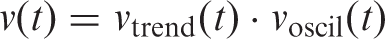
Any model of vection responding must therefore be capable of simulating both supra- and subthreshold vection experiences during continuous periods of visual motion stimulation. Accordingly, OPVM includes a threshold (θ) that demarks ON and OFF vection periods (ON periods occur whenever the modeled response exceeds the threshold for reporting a conscious experience vection).

Vection response output at time t during the trial (i.e., $V (t)$ ) is described by the following formula (with 1 and 0 representing ON and OFF vection periods, respectively):

V (t) = {\begin{matrix} 1 if v (t) \geq θ \\ 0 otherwise \end{matrix}

where

v (t)

describes internal state regarding the potential for the participant to experience vection, and θ is the threshold for reporting a conscious experience of vection.

We also employed a function $v_{trend} (t)$ that increased this potential gradually over time (to satisfy aforementioned Properties 1 and 2), as well as a periodic function $v_{oscil} (t)$ (to satisfy aforementioned Property 3):

v (t) = v_{trend} (t) \cdot v_{oscil} (t)

Directly after the start of the stimulus motion $(t = 0)$ , the vection response output $V (t)$ should be 0 (i.e., only object motion should be perceived at this time). $v (t)$ should then increase over time, eventually starting to plateau following expected vection saturation. Thus, we set the function $v_{trend} (t)$ as follows:

v_{trend} (t) = 1 - exp (- α t) (α > 0)

where the parameter α controls the latency to vection onset through

v_{trend} (t)

α

depends on visual motion stimulation S (which is regarded as the inducing potential of the optic flow). When there is no visual motion stimulation (

S = 0

), then

α (0)

will be

0

. However, when a vection inducing motion stimulus is presented (

S > 0

), then

α (S) > 0

. S and

α (S)

both increase with the vection inducing potential of the optic flow (e.g., they should increase as the size of the optic flow pattern increases—Dichgans & Brandt, 1978). As

α (S)

increases, the acceleration rate of

v_{trend}

also increases, which should result in shorter onsets and stronger magnitudes of vection responding. This is how the relationship between the visual motion stimulation and vection responding was incorporated into the model.

To model the alternation between ON and OFF vection reporting periods, we used a simple sinusoidal function:

v_{oscil} (t) = \frac{sin (2 π t / T) + β}{1 + β} (β > 1)

where T is the period of the oscillation during the plateau phase and β controls the value of the oscillation center. To perceive optic flow as being due to self-motion, it has been speculated that the system would need to first inhibit the default visual processing which is responsible for normally perceiving object or scene motion (e.g., Palmisano, Barry, De Blasio & Fogarty, 2016). The β and T values in this model control the oscillation between ON and OFF vection responding. It was proposed that they might represent the degree of inhibition of object motion processing (so as to instead favor self-motion processing) and the amount of time such inhibition is successful over the course of the “trial,” respectively.

Our mathematical model of vection (OPVM) was thus created by multiplying these two functions, $v_{trend} (t)$ and $v_{oscil} (t)$ . An example of the behavior of this model can be seen in Figure 1. The equation is able to satisfy all three of the vection properties identified previously in Constructing the Mathematical Model section. Values of $v_{trend} (t) and v_{oscil} (t)$ can range from 0 to 1. The internal potential $v (t)$ is therefore also able to vary from 0 to 1.

Figure 1.

The Oscillating Potential Vection Model (OPVM). The horizontal black arrows indicate “TIME” from the stimulus onset. The black fluctuating sinusoidally curved line indicates the simulated internal state of the participant over time. Whenever this curved line exceeds the threshold indicated by the green dashed line, vection will be reported (the onset of reported vection can therefore be estimated as the first time the curved line cuts the threshold). The tan boxes in the figure indicate “with vection periods.” Thus, the total size of these saw-toothed tan areas can be converted into an estimate of the overall vection magnitude for the trial.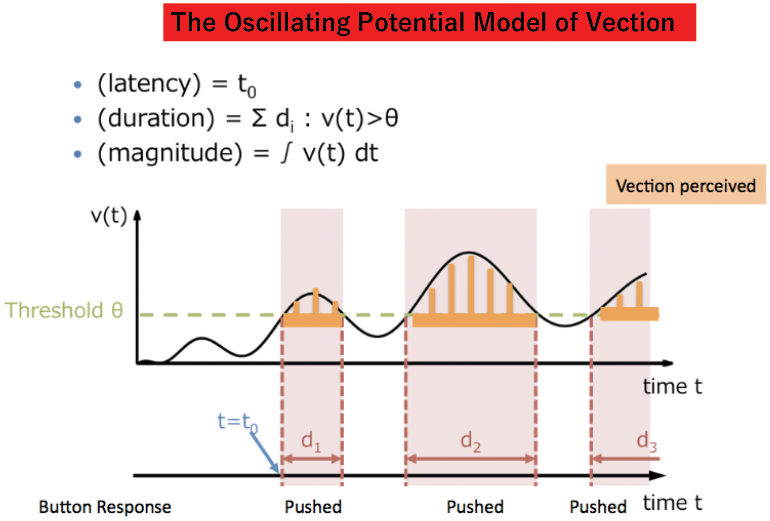

Modeling Empirically Observed Individual Differences

In this section, we will introduce and explain our mathematical model. Each parameter involved in the model (α, β, T, and θ) is important in determining the subjective vection response output ( $V (t)$ ). Figure 2(a) shows the simulated internal potential and resulting vection response output when the values of α, β, T, and θ are 0.1, 3, 10, and 0.6, respectively. As $α$ increases from 0.1 to 1 in Figure 2(b), the simulated vection onset latency can be seen to decrease. When β is reduced from 3 to 1.2 in Figure 2(c), the duration of the ON periods are reduced (e.g., compared with Figure 2(a)). The value of T can also be seen to affect the duration of ON and OFF periods. As T increases from 10 to 20, the initial ON duration increases and the frequency of switching between ON and OFF periods decreases (see Figure 2(d)). By modifying the values of these parameters, it should therefore be possible to model empirically observed individual differences in human vection responding.

Figure 2.

Examples of OPVM behavior with different α, β, T, and θ parameter sets. The horizontal and vertical axes are time and the value of $v (t)$ , respectively. The simulated participant experiences vection when $v (t) > θ$ (indicated by bold lines on the horizontal axes). Please see the main text for descriptions of a)-d) above.

Choosing the Vection Indices to Model

We next used OPVM response output to reconstruct the typical vection indices obtained in human laboratory experiments. In the past, the three most commonly employed measures of vection³ obtained in such studies have been (a) the latency to vection onset (i.e., the delay between the start of the visual motion stimulation and the observer’s first reported experience of illusory self-motion), (b) the total duration of the vection (i.e., the total amount of time that the observer reported experiencing vection during the trial), and (c) magnitude estimates or ratings of the vection experience (e.g., verbal ratings using a linear scale from 0 = no vection to 100 = very strong vection) (see Figure 3).

Figure 3.

A schematic illustration of the three vection measures: latency, duration, and magnitude. The horizontal black arrow indicates “TIME” between the onset and offset of the stimulus presentation. Boxes 1, 2, and 3 indicate “with vection periods” and the spaces between them indicate “vection dropouts”.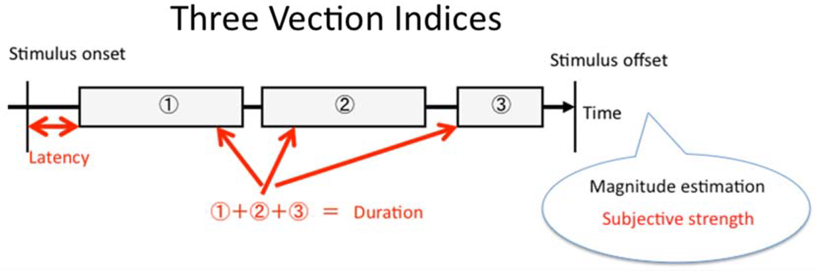

In our review of the recent literature, we found more than 50 papers where all three of these measures were obtained in the same experiment (see Allison, Ash, & Palmisano, 2014; Apthorp & Palmisano, 2014; Bonato & Bubka, 2006; Bonato, Bubka, Palmisano, Phillip, & Moreno, 2008; Brandt et al., 1973; Bubka & Bonato, 2010; Bubka et al., 2008; Gurnsey, Fleet, & Potechin, 1998; Guterman, Allison, Palmisano, & Zacher, 2012; Keshavarz et al., 2015; Keshavarz, Speck, Haycock, & Berti, 2017; Kim & Palmisano, 2008, 2010a; Mohler, Thompson, Riecke, & Bülthoff, 2005; Nakamura, 2006, 2010, 2012, 2013a, 2013b, 2013c, 2013d, 2013e; Nakamura, Palmisano, & Kim, 2016; Nakamura, Seno, Ito, & Sunaga, 2010, 2013; Nakamura & Shimojo, 1998, 1999, 2003; Ogawa, Ito, & Seno, 2015; Ogawa & Seno, 2014; Ogawa, Seno, Matsumori, & Higuchi, 2015; Palmisano, 1996; Palmisano, Burke, & Allison, 2003; Palmisano & Chan, 2004; Palmisano, Gillam, & Blackburn, 2000; Palmisano & Kim, 2009; Palmisano et al., 2011, 2015; Palmisano, Summersby, Davies & Kim, 2016; Riecke et al., 2006, 2009; Riecke, Feuereissen, Rieser, & McNamara, 2011; Sasaki, Seno, Yamada, & Miura, 2012; Seno, Abe, & Kiyokawa, 2013; Seno & Fukuda, 2012; Seno, Funatsu, & Palmisano, 2013; Seno, Ito, & Sunaga, 2009, 2010, 2011; Seno, Ito, Sunaga, & Palmisano, 2012; Seno, Kitaoka, & Palmisano, 2013; Seno & Palmisano, 2012; Seno, Palmisano, & Ito, 2011; Seno, Palmisano, Ito, & Sunaga, 2012; Shirai, Imura, Tamura, & Seno, 2014; Shirai, Seno, & Morohashi, 2012; Tamada & Seno, 2015; Tarita-Nistor, González, Spigelman, & Steinbach, 2006).

While other studies did not obtained all three measures together, most obtained at least one or more of them⁴ (e.g., Allison, Zacher, Kirollos, Guterman, & Palmisano, 2012; Andersen & Braunstein, 1985; Ash & Palmisano, 2012; Ash, Palmisano, Apthorp, & Allison, 2013; Ash, Palmisano, Govan, & Kim, 2011; Ash, Palmisano, & Kim, 2011; Becker, Raab, & Jürgens, 2002; Brandt, Dichgans, & Büchele, 1974; Brandt, Wist, & Dichgans, 1975; Delorme & Martin, 1986; Diels, Ukai, & Howarth, 2007; Fushiki, Takata, & Watanabe, 2000; Giannopulu & Lepecq, 1998; Haibach, Slobounov, & Newell, 2009; Held, Dichgans, & Bauer, 1975; Howard & Heckmann, 1989; IJsselsteijn, de Ridder, Freeman, Avons, & Bouwhuis, 2001; Ishida, Fushiki, Nishida, & Watanabe, 2008; Ito & Shibata, 2005; Ito & Takano, 2004; Ji, So, & Cheung, 2009; Jürgens et al., 2016; Kano, 1991; Kennedy, Hettinger, Harm, Ordy, & Dunlap, 1996; Kim & Khuu, 2014; Kim, Palmisano, & Bonato, 2012; Lubeck, Bos, & Stins, 2015; Ohmi & Howard, 1988; Ohmi, Howard, & Landolt, 1987; Palmisano, 2002; Palmisano, Allison, & Howard, 2006; Palmisano, Apthorp, Seno, & Stapley, 2014; Palmisano, Bonato, Bubka, & Folder, 2007; Palmisano, Kim, & Freeman, 2012; Palmisano, Mursic, & Kim, 2017; Post, 1988; Previc & Donnelly, 1993; Riecke & Feuereissen, 2012; Riecke, Freiberg, & Grechkin, 2015; Riecke & Jordan, 2015; Seno, Palmisano, Ito, & Sunaga, 2013; Seno, Palmisano, Riecke, & Nakamura, 2015; Tanahashi, Ujike, & Ukai, 2012; Tarita-Nistor, González, Markowitz, Lillakas, & Steinbach, 2008; Telford & Frost, 1993; Telford, Spratley, & Frost, 1992; Thurrell & Bronstein, 2002; Wong & Frost, 1981).

In these laboratory studies, the human observers were exposed to patterns of optic flow. Then, they typically had to press a button when they first experienced vection and hold this button down as long as this experience continued (releasing the button if the vection “dropped out” and pressing it again if the experience returned). The observers would then also typically provide a magnitude rating of the vection experience for that trial after the display motion had ceased.⁵

Reconstructing Vection Onset, Duration, and Magnitude From OPVM Response Output

We next used the OPVM response output to reconstruct each of these vection measures (onset, duration, and magnitude). Since a conscious vection experience occurs whenever $v (t) \geq θ$ , the first instance of $v (t) \geq θ$ in a simulation trial was used as the onset of vection. The total duration of vection was then calculated by summing all of the times in the particular simulation trial when $v (t) \geq θ$ . And finally, an estimate of the vection magnitude for the trial was calculated by integrating the area that the $v (t)$ function covers above the threshold line.

Testing OPVM

To investigate OPVM, we next conducted a large-scale virtual vection experiment. The three simulated response measures (onset latency, duration, and magnitude) were generated for each of the trials in this virtual experiment. Afterward, we compared this simulated response data with real data obtained previously in seven different vection experiments.

Virtual Vection Experiment

OPVM was used to simulate a virtual vection experiment consisting of 10,000 trials. The aim was to generate vection onset, duration, and magnitude response data which displayed individual differences similar to those commonly seen in human participants (i.e., due to their different sensitivities to vection, different response biases, etc.). To this end, the values of each parameter used in the simulation were randomly drawn from uniform distributions—except for α, which was drawn from a log-uniform distribution for each virtual trial. These uniform (other than α) and log-uniform (in the case of α) distributions ranged between $0.01$ and $1$ for α, $0$ and $5$ for β, $3$ and $20$ for T, and $0$ and $1$ for θ. While θ was free to span all possible values between 0 and 1, the ranges of α and T were determined during earlier pilot simulations. The value of α was chosen from a log-uniform distribution since this parameter has an exponential effect on the behavior of $v (t)$ . The size of $β$ was limited, because at larger values, there would be no simulated vection dropouts (i.e., instead, the range of βwe chose allowed for possible perceptual alternations between vection ON and OFF periods).

Results of the Virtual Experiment

The vection onset, duration, and magnitude data generated by OPVM for each of the 10,000 simulated trials is shown in Figure 4. These data are plotted as the correlations between (a) vection latency and magnitude, (b) vection duration and magnitude, and (c) vection latency and duration.

Figure 4.

The top three panels show the relationships between the virtual vection onset, duration, and magnitude responses generated by OPVM (only the first 1,000 of the total 10,000 trials are shown here for the sake of visibility). Significance levels are all p < .001. The bottom three panels show their corresponding heat maps. Intensity indicates the density of data points (i.e., brighter cells include more data points).

High correlations were found between all three of these simulated vection indices. In this analysis, “no vection” responses were treated as having a duration of 0 s and an onset latency of 40 s. In trials where vection was experienced, the sum of the onset and duration values was always less than 40 s (since there was always a finite delay before vection was experienced and motion stimulation only lasted 40 s). This is the reason that no data points appear in the upper right field of the latency-duration plot (Figure 4). Thus, these latency and duration data were not fully independent of each other (they were at least partially methodologically dependent on each other).

OPVM Performance Compared With Laboratory Vection Data

To further test the model, we next compared the simulated vection data (discussed in the Testing OPVM section) with real vection data obtained in seven different laboratory experiments. This real data consisted of human vection onset latency, duration, and magnitude responses. The details of these laboratory experiments are described in the following subsections.

Laboratory Experiments

Five out of these seven laboratory experiments had been published as scientific articles (in either English or Japanese—see Ogawa, Ito, & Seno, 2015; Ogawa & Seno, 2016; Ogawa, Seno, Matsumori, & Higuchi, 2015; Seno & Nagata, 2016; Seno, Ogawa, Tokunaga, & Kanaya, 2016). The remaining two experiments have yet to be published as papers. However, they have been both presented at international conferences (ICP: Ogawa, Seno, Ito, & Okajima, 2016; VSAC: Seno, Palmisano, & Nakamura, 2016).

Human participants

These experimental data were obtained from 107 different individuals (who were undergraduate students, graduate students, as well as staff and faculty members of Kyushu University). Participants reported no health issues at the time of testing. They had either normal or corrected to normal vision and no history of vestibular system diseases. While some of the authors of this article were participants, they did not know the purpose of these studies at the time of testing. Written informed consent was obtained from all participants prior to testing.

Apparatus

The vection stimuli were generated by and controlled via computers (MacBook Pro, MD101J/A, Apple Inc., Cupertino, CA; or ALIENWARE M18x, Dell Inc., Round Rock, TX) and presented on a 65-in. plasma display (3D VIERA TH-65AX800, Panasonic Corporation, Osaka, Japan) which had a resolution of 1920 × 1080 pixels and a refresh rate of 60 Hz. These experiments were all conducted in a dark room and participants always sat on a rocking chair to enhance their vection experience. No chin-rests or head-rests were used. Viewing distance to the display was held constant at approximately 57 cm across all of these experiments.

Stimuli

Two different types of experimental stimulus displays were used. In some experiments, a radially expanding optic flow stimulus was used, whereas in the remainder, a vertical optic flow stimulus was used. In both cases, these visual motion displays subtended a visual area of 100 (horizontal) × 80 (vertical) degrees² and the stimulus motion always lasted 40 s. The stimulus motion completely filled the display. Thus, the size of the stimulus and the display were approximately the same. The radially expanding pattern of optic flow consisted of white dots (38 cd/m²) presented on a black background (0 cd/m²). This display simulated forwards self-motion in depth at 16 m/s relative to a 3D cloud of 16,000 randomly positioned dots (see Figure 5, Top). As individual dots disappeared off the edges of the screen, they were moved back in depth to the far depth plane, thereby creating an endless optic flow display. Approximately 1,240 dots were visible in each frame, with each dot subtending a visual angle of 0.03° to 0.05° (their size remained constant as their simulated distances from the observer changed). Since these dots did not form a density gradient, motion perspective was the only cue to motion in depth. The second stimulus display presented the constant upward motion of a black grid (0 cd/m²) on a uniform white background (38 cd/m²)—it simulated downward self-motion at 18°/s (see Figure 5, Bottom). One side of each square in this rectangular grid subtended approximately 8° in visual angle.

Figure 5.

Schematic illustrations of the two types of stimuli used in the experiments in this article. (Top) Radially expanding optic flow. (Bottom) A vertically moving grid pattern.

Procedure

Participants observed these vection-inducing stimuli while sitting on a rocking chair inside a dark viewing chamber. Their task was (a) to press a button when they first experienced illusory self-motion and (b) to keep this button depressed as long as the experience continued (which provided data about both the onset latency and the duration of vection). After each stimulus presentation, they also had to report the subjective strength of their vection experience using 101-point rating scale (from 0 = no vection to 100 = very strong vection). Each stimulus display condition was repeated four times in each experiment. The 317 data sets used in this analyses were the result of testing 1,268 discrete vection trials. Each of the individual data sets consisted of the average onset, duration, and magnitude values obtained for a single subject in one experiment.

Results

Laboratory vection data

Correlational analyses were conducted on 317 discrete sets of laboratory-obtained vection data. Figure 6 shows the relationships between the three different vection measures. All combinations of these measures were found to generate significant correlations (latency–magnitude, R (317) = −.55, p < .001; duration–magnitude, R (317) = .66, p < .001; latency–duration, R (317) = −.79, p < .001; see also Figure 4). These three correlation coefficients were significantly different to each other (z = 2.13, p = .03, z = 3.51, p < .001, and z = 3.51, p < .001, respectively, for latency-magnitude and duration-magnitude, duration-magnitude and latency-duration, and latency-magnitude and latency-duration). Magnitude ratings were found to account for 30% of the variability in vection onset latency and 44% of the variability in vection duration. The strongest relationship was found for the two time course measures—with vection duration accounting for ∼62% of the variability in vection onset latency responses. The strength of this relationship between vection onset and duration was presumably due in part to the unavoidable trade-off between the two time course measures (as vection onset latency increased, vection duration typically decreased. As noted earlier, these latency and duration data were at least partially methodologically dependent on each other).

Figure 6.

The top three panels show the vection onset, duration, and magnitude responses obtained in the seven laboratory experiments. The bottom three panels show their corresponding heat maps. Intensity again indicates the density of data points (i.e., brighter cells include more data points).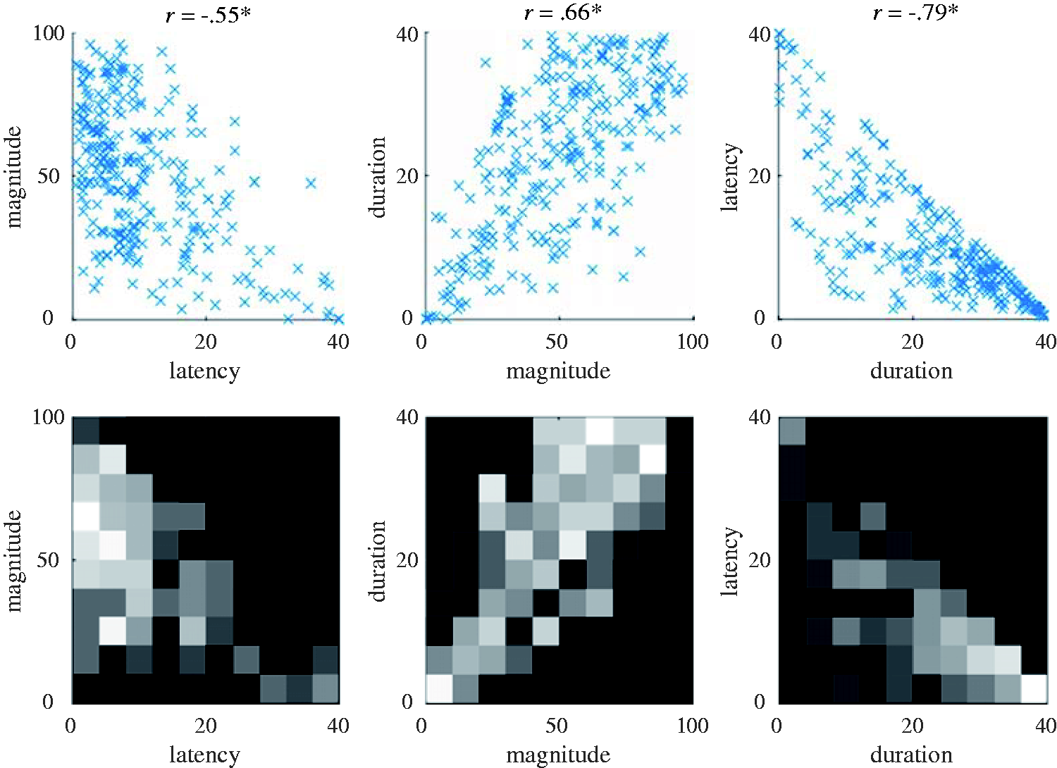

Comparison of OPVM and laboratory results

When we compared the corresponding virtual and laboratory vection data with each other, we noticed a number of similarities in their distributions. To better visualize these similarities between OPVM-generated and human data, we superimposed data points from our earlier virtual (Figure 4, Top) and laboratory (Figure 6, Top) plots—thereby creating the new Figure 7.⁶

Figure 7.

Comparisons of OPVM’s simulated data (blue) with the empirical data (red) obtained in the laboratory vection experiments.

This new figure depicts the relationships between latency and magnitude, magnitude and duration, as well as latency and duration for the OPVM and laboratory-based vection response data. Both the OPVM and human data were found to produce (a) significant positive relationships between magnitude and duration (R = .87 and R = .66, respectively), (b) significant negative relationships between magnitude and latency (R = −.56 and R = −.55, respectively), and (c) significant negative relationships between latency and duration (R = −.67 and R = −.79).

OPVM also appeared to be successful in generating substantial variability in the responding. Indeed, this variability in responding appeared to mimic (at least superficially) some of the individual differences seen in the human responding. However, OPVM’s responding appeared to be less variable than the human responding. These discrepancies in response variability appeared to be more obvious in the latency versus magnitude and the duration versus magnitude plots (compared with the latency versus duration plot). These discrepancies will be discussed in detail later.

Discussion

In this article, we developed and tested a model of responding to visually induced vection, the OPVM. OPVM was constructed based on three well-documented properties of the vection experience: (a) that there is a finite delay before the reported onset of vection, (b) that there is a subsequent increase of reported vection magnitude over time until vection responding eventually plateaus, and (c) that vection dropouts are reported to occur (after vection induction and before the display motion ceases). Next, in our 10,000 virtual trial simulation experiment, we attempted to model not only these three properties of vection but also commonly observed individual differences in vection responding (by altering the values of key parameters of OPVM: α, β, T, and θ). Vection onset latency, duration, and magnitude estimates were reconstructed (based on the OPVM response outputs) for each virtual trial. Finally, we compared the performance of our model with the results of previous laboratory studies which obtained the same vection measures. Statistical analyses of the real and model-based vection data indicated that all three measures correlated significantly with each other.

Our results demonstrate that both overall and specific vection responding (including individual differences) can be described quite well by OPVM. However, there also appeared to be some notable inconsistencies between the real and simulated vection response data. These can best be seen in the Latency-Magnitude correlation (Figures 7, Left) and the Duration-Magnitude correlation (Figure 7, Middle) plots. In the latter case, magnitude ratings appeared to be considerably larger for longer vection durations during simulation, whereas the equivalent relationship between magnitude and duration was noticeably weaker for the real vection data. We speculate that this particular discrepancy might reflect idiosyncrasies in human responding rather than potential inadequacies of OPVM. During the vection experiments, participants observed each visual motion display for 40 s and only provided their magnitude ratings after the display motion ceased. It is likely that the magnitude ratings made by our human participants did not accurately reflect the average strength of their vection experience across the entire trial but instead were biased by stronger vection experiences they had toward the end of the trial. If this explanation is valid, then this real versus simulated vection data discrepancy might reflect a recency effect.⁷ Future work should thus be aimed at incorporating such human response characteristics (particularly those common when making perceptual judgments) into OPVM.

To better understand and predict the conscious experience of vection, OPVM will need to be further developed and refined. In the current version of OPVM, we utilized sinusoidal and exponential functions in an attempt to model the experience of vection. However, these are rather simple mathematical functions. It is likely that more complex mathematical functions may be required to improve the model (e.g., it is highly likely that temporal changes in both human perception and responding may be different from the sinusoidal changes currently incorporated into OPVM). This will undoubtedly require further empirical investigations of vection (obtaining new data by using different display manipulations and other measurement methods). For example, several previous studies have had participants press different buttons that correspond to the subjective magnitude of the vection they are experiencing at the time (no vection, weak, modest, and strong) and then examined the total amount of time that each of these buttons was depressed during the trial (e.g., Mohler et al., 2005; Riecke et al., 2006, 2009, 2011; Seya, Shinoda, & Nakaura, 2015; Seya, Tsuji, & Shinoda, 2014; Seya, Yamaguchi, & Shinoda, 2015). The accumulation of these magnitude values over entire stimulus presentation period was then used to assess the overall vection experience. Other studies have used joysticks, slider devices, or levers to collect continuous ratings of vection magnitude over the entire course of each trial (e.g., Apthorp, Nagle, & Palmisano, 2014; Apthorp & Palmisano, 2014; Berthoz, Pavard, & Young, 1975; Bonato & Bubka, 2006; Bubka et al., 2008; Kim & Palmisano, 2010b; Palmisano, 2002; Seno, Yamada, & Palmisano, 2012; Telford et al., 1992; Trutoiu, Mohler, Schulte-Pelkum, & Bülthoff, 2009; Weech & Troje, 2017). By employing similar methods, we might be able to analyze the tendencies of the temporal change in vection strength more precisely and incorporate the results into OPVM. Vection strength and time averaging should therefore be further examined in future.

As noted earlier, another potential issue with the current investigation was that the latency and duration data (both reported in seconds) were not fully independent of each other. As in the majority of past laboratory studies, these data were at least partially methodologically dependent on each other (because the trial duration was fixed; therefore, longer vection onsets would be more likely to be associated with shorter vection durations—even factoring in the possibility of subsequent vection dropouts). An alternative way to examine the relationships between these temporal vection measures might be to recode the latter duration measure as a percentage of the time that vection was experienced as a function of the entire stimulus presentation period (as has been recently suggested by Keshavarz et al., 2017). For example, a vection experience lasting 30 s during a 40-s stimulus presentation period would be recoded as a % duration value of 75. Reexamining our model with this and other alternative vection response measures should therefore also be a future task for us.⁸

Furthermore, vection is not restricted to vision, but vection can also be induced by stimulating other sensory modalities, for example, auditory vection (e.g., Väljamäe & Sell, 2014; Väljamäe, 2009, for review) and cutaneous vection (Murata, Seno, Ozawa, & Ichihara, 2014). In the development of OPVM, only the properties of visually induced vection were considered. However, there are similarities between the vection experiences induced by visual and other perceptual modalities. Thus, it is possible that the model could be applied or extended to vection induced by other nonvisual modalities.

Although the OPVM has room for improvement as noted earlier, the current version is capable of describing the reported experience of vection quite well (despite its rather simplistic component functions). OPVM therefore has the potential to be a useful tool in understanding both the overall and specific experiences of vection.

Footnotes

Declaration of Conflicting Interests

The author(s) declared no potential conflicts of interest with respect to the research, authorship, and/or publication of this article.

Funding

The author(s) disclosed receipt of the following financial support for the research, authorship, and/or publication of this article: This work was supported by the Program to Disseminate Tenure Tracking System to T.S., and by JSPS KAKENHI Grant Numbers JP26700016 and 17K12869 (Grants-in-Aid for Young Scientists A and Young Scientists B) to T.S. and Y.F., JP15K21484 and JP26381000 (Grants-in-Aid for Young Scientists B and Scientific Research C) to H.K., from Ministry of Education, Culture, Sports, Science and Technology of Japan. Part of this work was carried out under the Cooperative Research Project Program of the Research Institute of Electrical Communication, Tohoku University.

Notes

Author Biographies

Takeharu Seno: is an associate professor in the Faculty of Design at Kyushu University, in Fukuoka, Japan. His research topic has been “Vection” for more than 15 years. He became interested in vection while working on his PhD under the supervision of Professor Takao Sato at the University of Tokyo and later on as a post-doctoral fellow working with Professor Hiroyuki Ito at Kyushu University. Also, he studied and worked in the University of Wollongong under the supervision of Professor Stephen Palmisano, in Wollongong, Australia.

Ken-ichi Sawai: is a research associate in Graduate Schools for Law and Politics at The University of Tokyo. He received a PhD in Information Science and Technology from The University of Tokyo. His main research interests are mathematically understanding the human perception and cognition.

Hidetoshi Kanaya: is an assistant professor in the Faculty of Human Informatics, Aichi Shukutoku University, Japan. He received PhD in Psychology from The University of Tokyo under the supervision of Professor Takao Sato. His research interests include visual perception (motion, depth), attention, self-motion, multimodal perception and action, and embodied cognition.

Toshihiro Wakebe: is a lecturer at Fukuoka Jo Gakuin University in Fukuoka, Japan. He has investigated in human memory based on experimental psychology and cognitive neuroscience. He got a PhD in psychology from the University of Tokyo (supervisor: Yohtaro Takano) and later devoted himself to research on memory and plasticity using rTMS, tACS, ECoG, and EEG at Department of Medicine, the University of Tokyo (supervisor: Katsuyuki Sakai).

Masaki Ogawa: is a researcher of Faculty of Design, Kyushu University, Japan. He received his Ph.D in Design from Kyushu University in 2015. His research interests are visual attention and illusory self-motion perception (vection).

Yoshitaka Fujii: is a post-doctoral fellow at Ritsumeikan University. His insterets are in depth pereception, stereo vision and vection. He recieved a PhD from Tokyo Institute of Technology (Tokyo, Japan), and worked in York University (Canada), Tokyo institute of technology, Kanazawa Institute of Technology and Kyushu University (Japan).

Stephen Palmisano: is an associate professor in the School of Psychology at the University of Wollongong. His research investigates how people perceive their own self-motions (both real and illusory) and how having two eyes benefits their perception of depth. Stephen became interested in both areas of research while working on his PhD under the supervision of Scientia Professor Barbara Gillam at UNSW and later on as a post-doctoral fellow working with Distinguished Research Professor Ian P. Howard at the Centre for Vision Research, York University, Canada.

References

Adelson

E. H.

Bergen

J. R.

(1985) Spatiotemporal energy models for the perception of motion. Journal of the Optical Society of America A 2: 284–299. doi: 10.1364/JOSAA.2.000284.

Allison

R. S.

Ash

Palmisano

(2014) Binocular contributions to linear vertical vection. Journal of Vision 14: 1–23. doi:10.1167/14.12.5.

Allison

R. S.

Howard

I. P.

Zacher

J. E.

(1999) Effect of field size, head motion, and rotational velocity on roll vection and illusory self-tilt in a tumbling room. Perception 28: 299–306. doi: 10.1068/p2891.

Allison

R. S.

Zacher

J. E.

Kirollos

Guterman

P. S.

Palmisano

(2012) Perception of smooth and perturbed vection in short-duration microgravity. Experimental Brain Research 223: 479–487. doi: 10.1007/s00221-012-3275-5.

Andersen

G. J.

Braunstein

M. L.

(1985) Induced self-motion in central vision. Journal of Experimental Psychology: Human Perception and Performance 11: 122–132. doi: 10.1037/0096-1523.11.2.122.

Apthorp

Nagle

Palmisano

(2014) Chaos in balance: Non-linear measures of postural control predict individual variations in visual illusions of motion. PLoS One 9: e113897, 1–22. doi:10.1371/journal.pone.0113897.

Apthorp

Palmisano

(2014) The role of perceived speed in vection: Does perceived speed modulate the jitter and oscillation advantages? PLoS One 9: e92260, 1–14. doi:10.1371/journal.pone.0092260.

Ash

Palmisano

(2012) Vection during conflicting multisensory information about the axis, magnitude and direction of self-motion. Perception 41: 253–267. doi: 10.1068/p7129.

Ash

Palmisano

Apthorp

Allison

R. S.

(2013) Vection in depth during treadmill walking. Perception 42: 562–576. doi: 10.1068/p7449.

10.

Ash

Palmisano

Govan

D. G.

Kim

(2011) Display lag and gain effects on vection experienced by active observers. Aviation, Space, and Environmental Medicine 82: 763–769. doi: 10.3357/ASEM.3026.2011.

11.

Ash

Palmisano

Kim

(2011) Vection in depth during consistent and inconsistent multisensory stimulation. Perception 40: 155–174.

12.

Becker

Raab

Jürgens

(2002) Circular vection during voluntary suppression of optokinetic reflex. Experimental Brain Research 144: 554–557.

13.

Berthoz

Pavard

Young

L. R.

(1975) Perception of linear horizontal self-motion induced by peripheral vision (linearvection): Basic characteristics and visual-vestibular interactions. Experimental Brain Research 23: 471–489.

14.

Bles

(1981) Stepping around circular vection and coriolis effects. In: Longand

Baddeley

(eds) Attention and performance IX, Hillsdale, NJ: Lawrence Erlbaum Associates, pp. 47–61.

15.

Bonato

Bubka

(2006) Chromaticity, spatial complexity, and self-motion perception. Perception 35: 53–64.

16.

Bonato

Bubka

Palmisano

Phillip

Moreno

(2008) Vection change exacerbates simulator sickness in virtual environments. Presence: Teleoperators and Virtual Environments 17: 283–292.

17.

Brandt

Dichgans

Büchele

(1974) Motion habituation: Inverted self-motion perception and optokinetic after-nystagmus. Experimental Brain Research 21: 337–352.

18.

Brandt

Dichgans

Koenig

(1973) Differential effects of central versus peripheral vision on egocentric and exocentric motion perception. Experimental Brain Research 16: 476–491.

19.

Brandt

Wist

E. R.

Dichgans

(1975) Foreground and background in dynamic spatial orientation. Perception & Psychophysics 17: 497–503.

20.

Bubka

Bonato

(2010) Natural visual-field features enhance vection. Perception 39: 627–635.

21.

Bubka

Bonato

Palmisano

(2008) Expanding and contracting optic-flow patterns and vection. Perception 37: 704–711.

22.

Carpenter-Smith

T. R.

Futamura

R. G.

Parker

D. E.

(1995) Inertial acceleration as a measure of linear vection: An alternative to magnitude estimation. Perception & Psychophysics 57: 35–42.

23.

Cuturi

L. F.

MacNeilage

P. R.

(2014) Optic flow induces nonvisual self-motion aftereffects. Current Biology 24: 2817–2821.

24.

D’Amour

Bos

J. E.

Keshavarz

(2017) The efficacy of airflow and seat vibration on reducing visually induced motion sickness. Experimental Brain Research 235: 2811–2820.

25.

de Graaf

Wertheim

A. H.

Bles

(1991) The Aubert-Fleischl paradox does appear in visually induced self-motion. Vision Research 31: 845–849.

26.

Delorme

Martin

(1986) Roles of the retinal periphery and depth periphery in linear vection and visual control of standing in humans. Canadian Journal of Psychology 40: 176–187.

27.

Dichgans

Brandt

(1978) Visual-vestibular interaction: Effects on self-motion perception and postural control. In: Held

Leibowitz

H. W.

Teuber

H.-L.

(eds) Handbook of sensory physiology Vol. 8, Berlin, Germany: Springer, pp. 755–804. . doi:10.1007/978-3-642-46354-9_25.

28.

Diels

Ukai

Howarth

P. A.

(2007) Visually induced motion sickness with radial displays: Effects of gaze angle and fixation. Aviation, Space, and Environmental Medicine 78: 659–665.

29.

Fushiki

Takata

Watanabe

(2000) Influence of fixation on circular vection. Journal of Vestibular Research 10: 151–155.

30.

Giannopulu

Lepecq

J. C.

(1998) Linear-vection chronometry along spinal and sagittal axes in erect man. Perception 27: 363–372.

31.

Gurnsey

Fleet

Potechin

(1998) Second-order motions contribute to vection. Vision Research 38: 2801–2816.

32.

Guterman

P. S.

Allison

R. S.

Palmisano

Zacher

J. E.

(2012) Influence of head orientation and viewpoint oscillation on linear vection. Journal of Vestibular Research 22: 105–116.

33.

Haibach

Slobounov

Newell

(2009) Egomotion and vection in young and elderly adults. Gerontology 55: 637–643.

34.

Held

Dichgans

Bauer

(1975) Characteristics of moving visual scenes influencing spatial orientation. Vision Research 15: 357–365.

35.

Hettinger

L. J.

Schmidt

Jones

D. L.

Keshavarz

(2014) Illusory self-motion in virtual environments. In: Hale

K. S.

Stanney

K. M.

(eds) Handbook of virtual environments: Design, implementation, and applications, 2nd ed. New York, NY: CRC Press, pp. 435–466.

36.

Howard

I. P.

(1982) Human visual orientation, New York, NY: John Wiley & Sons.

37.

Howard

I. P.

Heckmann

(1989) Circular vection as a function of the relative sizes, distances, and positions of two competing visual displays. Perception 18: 657–665.

38.

Howard

I. P.

Zacher

J. E.

Allison

R. S.

(1998) Post-rotatory nystagmus and turning sensations after active and passive turning. Journal of Vestibular Research 8: 299–312.

39.

Ihaya

Seno

Yamada

(2014) Più mosso: Fast self-motion makes cyclic action faster in virtual reality. Revista Latinoamericana de Psicología 46: 53–58.

40.

IJsselsteijn

de Ridder

Freeman

Avons

S. E.

Bouwhuis

(2001) Effects of stereoscopic presentation, image motion, and screen size on subjective and objective corroborative measures of presence. Presence: Teleoperators and Virtual Environments 10: 298–311.

41.

Ishida

Fushiki

Nishida

Watanabe

(2008) Self-motion perception during conflicting visual-vestibular acceleration. Journal of Vestibular Research 18: 267–272.

42.

Ito

Shibata

(2005) Self-motion perception from expanding and contracting optical flows overlapped with binocular disparity. Vision Research 45: 397–402.

43.

Ito

Takano

(2004) Controlling visually induced self-motion perception: Effect of overlapping dynamic visual noise. Journal of Physiological Anthropology and Applied Human Science 23: 307–311.

44.

J. T. T.

R. H. Y.

Cheung

R. T. F.

(2009) Isolating the effects of vection and optokinetic nystagmus on optokinetic rotation-induced motion sickness. Human Factors 51: 739–751.

45.

Jürgens

Kliegl

Kassubek

Becker

(2016) Optokinetic circular vection: A test of visual-vestibular conflict models of vection nascensy. Experimental Brain Research 234: 67–81.

46.

Kano

(1991) The perception of self-motion induced by peripheral visual information in sitting and supine postures. Ecological Psychology 3: 241–252.

47.

Kennedy

R. S.

Hettinger

L. J.

Harm

D. L.

Ordy

J. M.

Dunlap

W. P.

(1996) Psychophysical scaling of circular vection (CV) produced by optokinetic (OKN) motion: Individual differences and effects of practice. Journal of Vestibular Research 6: 331–341.

48.

Keshavarz

Hettinger

L. J.

Vena

Campos

J. L.

(2014) Combined effects of auditory and visual cues on the perception of vection. Experimental Brain Research 232: 827–836.

49.

Keshavarz

Riecke

B. E.

Hettinger

L. J.

Campos

J. L.

(2015) Vection and visually induced motion sickness: How are they related? Frontiers in Psychology 6. , 472, 1–11. doi:10.3389/fpsyg.2015.00472.

50.

Keshavarz

Speck

Haycock

Berti

(2017) Effect of different display types on vection and its interaction with motion direction and field dependence. i-Perception 8: 1–18. doi:10.1177/2041669517707768.

51.

Kim

Khuu

(2014) A new spin on vection in depth. Journal of Vision 14: 1–10. doi:10.1167/14.5.5.

52.

Kim

Palmisano

(2008) Effects of active and passive viewpoint jitter on vection in depth. Brain Research Bulletin 77: 335–342.

53.

Kim

Palmisano

(2010a) Visually mediated eye movements regulate the capture of optic flow in self-motion perception. Experimental Brain Research 202: 355–361.

54.

Kim

Palmisano

(2010b) Eccentric gaze dynamics enhance vection in depth. Journal of Vision 10: 1–11. doi:10.1167/10.12.7.

55.

Kim

Palmisano

Bonato

(2012) Simulated angular head oscillation enhances vection in depth. Perception 41: 402–414.

56.

Kruijff, E., Riecke, B., Trepkowski, C., & Kitson, A. (2015). Upper body leaning can affect forward self-motion perception in virtual environments. Proceedings of the 3rd ACM Symposium on Spatial User Interaction (pp. 103–112). New York, NY: ACM. doi:10.1145/2788940.2788943.

57.

Lepecq

J.-C.

Giannopulu

Baudonniere

P.-M.

(1995) Cognitive effects on visually induced body motion in children. Perception 24: 435–449.

58.

Lubeck

A. J. A.

Bos

J. E.

Stins

J. F.

(2015) Interaction between depth order and density affects vection and postural sway. PLoS One 10: e0144034, 1–12. doi:10.1371/journal.pone.0144034.

59.

McAnally

K. I.

Martin

R. L.

(2008) Sound localisation during illusory self-rotation. Experimental Brain Research 185: 337–340.

60.

Mergner

Schweigart

Müller

Hlavacka

Becker

(2000) Visual contributions to human self-motion perception during horizontal body rotation. Archives Italiennes de Biologie 138: 139–166.

61.

Miller

M. A.

O’Leary

C. J.

Allen

P. D.

Crane

B. T.

(2015) Human vection perception using inertial nulling and certainty estimation: The effect of migraine history. PLoS One 10. e0135335, 1–25. doi:10.1371/journal.pone.0135335.

62.

Mohler, B. J., Thompson, W. B., Riecke, B., & Bülthoff, H. H. (2005). Measuring vection in a large screen virtual environment. Proceedings of the 2nd ACM symposium on applied perception in graphics and visualization (pp. 103–109). New York, NY: ACM. doi:10.1145/1080402.1080421.

63.

Motoyoshi

Nishida

Sharan

Adelson

E. H.

(2007) Image statistics and the perception of surface qualities. Nature 447: 206–209.

64.

Murata

Seno

Ozawa

Ichihara

(2014) Self-Motion perception induced by cutaneous sensation caused by constant wind. Psychology 5: 1777–1782.

65.

Mursic

R. A.

Riecke

B. E.

Apthorp

Palmisano

(2017) The Shepard-Risset glissando: Music that moves you. Experimental Brain Research 235: 3111–3127.

66.

Nakamura

(2006) Effects of depth, eccentricity and size of additional static stimulus on visually induced self-motion perception. Vision Research 46: 2344–2353.

67.

Nakamura

(2010) Additional oscillation can facilitate visually induced self-motion perception: The effects of its coherence and amplitude gradient. Perception 39: 320–329.

68.

Nakamura

(2012) Effects of stimulus eccentricity on the perception of visually induced self-motion facilitated by simulated viewpoint jitter. Seeing & Perceiving 25: 647–654.

69.

Nakamura

(2013a) The minimum stimulus conditions for vection—Two- and four-stroke apparent motions can induce self-motion perception. Perception 42: 245–247.

70.

Nakamura

(2013b) Separate presentation of additional accelerating motion does not enhance visually induced self-motion perception. Multisensory Research 26: 277–285.

71.

Nakamura

(2013c) Effects of additional visual oscillation on vection under voluntary eye movement conditions—Retinal image motion is critical in vection facilitation. Perception 42: 529–536.

72.

Nakamura

(2013d) Visual jitter inhibits roll vection for an upright observer. Perception 42: 751–758.

73.

Nakamura

(2013e) Rotational jitter around the observer’s line of sight can facilitate visually induced perception of forward self-motion (forward vection). Multisensory Research 26: 553–560.

74.

Nakamura

Palmisano

Kim

(2016) Relative visual oscillation can facilitate visually induced self-motion perception. i-Perception 7: 1–18. doi:10.1177/2041669516661903.

75.

Nakamura

Seno

Ito

Sunaga

(2010) Coherent modulation of stimulus colour can affect visually induced self-motion perception. Perception 39: 1579–1590.

76.

Nakamura

Seno

Ito

Sunaga

(2013) Effects of dynamic luminance modulation on visually induced self-motion perception: Observers’ perception of illumination is important in perceiving self-motion. Perception 42: 153–162.

77.

Nakamura

Shimojo

(1998) Stimulus size and eccentricity in visually induced perception of horizontally translational self-motion. Perceptual and Motor Skills 87: 659–663.

78.

Nakamura

Shimojo

(1999) Critical role of foreground stimuli in perceiving visually induced self-motion (vection). Perception 28: 893–902.

79.

Nakamura

Shimojo

(2003) Sustained deviation of gaze direction can affect “inverted vection” induced by the foreground motion. Vision Research 43: 745–749.

80.

Nesti

Beykirch

K. A.

Pretto

Bülthoff

H. H.

(2015) Self-motion sensitivity to visual yaw rotations in humans. Experimental Brain Research 233: 861–869.

81.

Nordahl, R., Nilsson, N. C., Turchet, L., & Serafin, S. (2012). Vertical illusory self-motion through haptic stimulation of the feet. Proceedings of the IEEE VR Workshop on Perceptual Illusions in Virtual Environments (PIVE) (pp. 21–26). New York, NY: IEEE. doi:10.1109/PIVE.2012.6229796.

82.

Ogawa

Ito

Seno

(2015) Vection is unaffected by circadian rhythms. Psychology 6: 440–446.

83.

Ogawa

Seno

(2014) Vection is modulated by the semantic meaning of stimuli and experimental instructions. Perception 43: 605–615.

84.

Ogawa

Seno

(2016) Vection strength can be socially modulated through conformity to the reported perception of others. Transactions of the Virtual Reality Society of Japan 21: 23–29.

85.

Ogawa, M., Seno, T., Ito, H., & Okajima, K. (2016). Vection strength is determined by the subjective size of a visual stimulus modulated by amodal completion. Paper presented at the 31st International Congress of Psychology (ICP 2016), Pacifico Yokohama, Japan (July 2016).

86.

Ogawa

Seno

Matsumori

Higuchi

(2015) Twenty-hour sleep deprivation does not affect perceived vection strength. Journal of Behavioral and Brain Science 5: 550–560.

87.

Ohmi

Howard

I. P.

(1988) Effect of stationary objects on illusory forward self-motion induced by a looming display. Perception 17: 5–11.

88.

Ohmi

Howard

I. P.

Landolt

J. P.

(1987) Circular vection as a function of foreground-background relationships. Perception 16: 17–22.

89.

Palmisano

(1996) Perceiving self-motion in depth: The role of stereoscopic motion and changing-size cues. Perception & Psychophysics 58: 1168–1176.

90.

Palmisano

(2002) Consistent stereoscopic information increases the perceived speed of vection in depth. Perception 31: 463–480.

91.

Palmisano

Allison

R. S.

Howard

I. P.

(2006) Illusory scene distortion occurs during perceived self-rotation in roll. Vision Research 46: 4048–4058.

92.

Palmisano

Allison

R. S.

Kim

Bonato

(2011) Simulated viewpoint jitter shakes sensory conflict accounts of vection. Seeing & Perceiving 24: 173–200.

93.

Palmisano

Allison

R. S.

Schira

M. M.

Barry

R. J.

(2015) Future challenges for vection research: Definitions, functional significance, measures, and neural bases. Frontiers in Psychology 6: 1–15. doi:10.3389/fpsyg.2015.00193.

94.

Palmisano

Apthorp

Seno

Stapley

P. J.

(2014) Spontaneous postural sway predicts the strength of smooth vection. Experimental Brain Research 232: 1185–1191.

95.

Palmisano

Barry

R. J.

De Blasio

F. M.

Fogarty

J. S.

(2016) Identifying objective EEG based markers of linear vection in depth. Frontiers in Psychology 7: 1–11. doi:10.3389/fpsyg.2016.01205.

96.

Palmisano

Bonato

Bubka

Folder

(2007) Vertical display oscillation effects on forward vection and simulator sickness. Aviation, Space, and Environmental Medicine 78: 951–956.

97.

Palmisano

Burke

Allison

R. S.

(2003) Coherent perspective jitter induces visual illusions of self-motion. Perception 32: 97–110.

98.

Palmisano

Chan

A. Y. C.

(2004) Jitter and size effects on vection are immune to experimental instructions and demands. Perception 33: 987–1000.

99.

Palmisano

Gillam

B. J.

(1998) Stimulus eccentricity and spatial frequency interact to determine circular vection. Perception 27: 1067–1077.

100.

Palmisano

Gillam

B. J.

Blackburn

S. G.

(2000) Global perspective jitter improves vection in central vision. Perception 29: 57–67.

101.

Palmisano

Kim

(2009) Effects of gaze on vection from jittering, oscillating, and purely radial optic flow. Attention, Perception, & Psychophysics 71: 1842–1853.

102.

Palmisano

Kim

Freeman

T. C. A.

(2012) Horizontal fixation point oscillation and simulated viewpoint oscillation both increase vection in depth. Journal of Vision 12: 1–14. doi:10.1167/12.12.15.

103.

Palmisano

Mursic

Kim

(2017) Vection and cybersickness generated by head-and-display motion in the Oculus Rift. Displays 46: 1–8.

104.

Palmisano

Pinniger

G. J.

Ash

Steele

J. R.

(2009) Effects of simulated viewpoint jitter on visually induced postural sway. Perception 38: 442–453.

105.

Palmisano

Summersby

Davies

R. G.

Kim

(2016) Stereoscopic advantages for vection induced by radial, circular, and spiral optic flows. Journal of Vision 16: 1–19. doi:10.1167/16.14.7.

106.

Post

R. B.

(1988) Circular vection is independent of stimulus eccentricity. Perception 17: 737–744.

107.

Previc

F. H.

Donnelly

(1993) The effects of visual depth and eccentricity on manual bias, induced motion, and vection. Perception 22: 929–945.

108.

Riecke

B. E.

(2010) Compelling self-motion through virtual environments without actual self-motion—Using self-motion illusions (‘vection') to improve user experience in VR. In: Kim

J.-J.

(ed.) Virtual reality, New York, NY: InTech. 161–188. doi:10.5772/13150.

109.

Riecke, B. E., & Feuereissen, D. (2012). To move or not to move: Can active control and user-driven motion cueing enhance self-motion perception (“vection”) in virtual reality? Proceedings of the ACM Symposium on Applied Perception (pp. 17–24). New York, NY: ACM. doi:10.1145/2338676.2338680.

110.

Riecke

B. E.

Feuereissen

Rieser

J. J.

McNamara

T. P.

(2011) Spatialized sound enhances biomechanically-induced self-motion illusion (vection). Proceedings of the SIGCHI Conference on Human Factors in Computing Systems, Vancouver. 2799–2802. doi:10.1145/1978942.1979356.

111.

Riecke

B. E.

Freiberg

J. B.

Grechkin

T. Y.

(2015) Can walking motions improve visually induced rotational self-motion illusions in virtual reality? Journal of Vision 15: 1–15. doi:10.1167/15.2.3.

112.

Riecke

B. E.

Jordan

J. D.

(2015) Comparing the effectiveness of different displays in enhancing illusions of self-movement (vection). Frontiers in Psychology 6: 1–16. doi:10.3389/fpsyg.2015.00713.

113.

Riecke

B. E.

Schulte-Pelkum

Avraamides

M. N.

Von Der Heyde

Bülthoff

H. H.

(2006) Cognitive factors can influence self-motion perception (vection) in virtual reality. ACM Transactions on Applied Perception 3: 194–216. doi:10.1145/1166087.1166091.

114.

Riecke

B. E.

Väljamäe

Schulte-Pelkum

(2009) Moving sounds enhance the visually-induced self-motion illusion (circular vection) in virtual reality. ACM Transactions on Applied Perception 6: 1–27. doi: 10.1145/1498700.1498701.

115.

Rosenblatt

S. D.

Crane

B. T.

(2015) Influence of visual motion, suggestion, and illusory motion on self-motion perception in the horizontal plane. PLoS One 10: e0142109, 1–13. doi:10.1371/journal.pone.0142109.

116.

Sasaki

Seno

Yamada

Miura

(2012) Emotional sounds influence vertical vection. Perception 41: 875–877.

117.

Sato, H., Motoyoshi, I., & Sato, T. (2013). Perception of global trend from dynamic stimuli. Paper presented at the Vision Sciences Society (VSS) 13th Annual Meeting, Naples, Florida, USA (May 2013).

118.

Sauvan

X. M.

Bonnet

(1993) Properties of curvilinear vection. Perception & Psychophysics 53: 429–435.

119.

Sauvan

X. M.

Bonnet

(1995) Spatiotemporal boundaries of linear vection. Perception & Psychophysics 57: 898–904.

120.

Seno

Abe

Kiyokawa

(2013) Wearing heavy iron clogs can inhibit vection. Multisensory Research 26: 569–580.

121.

Seno

Fukuda

(2012) Stimulus meanings alter illusory self-motion (vection)—Experimental examination of the train illusion. Seeing & Perceiving 25: 631–645.

122.

Seno

Funatsu

Palmisano

(2013) Virtual swimming—Breaststroke body movements facilitate vection. Multisensory Research 26: 267–275.

123.

Seno

Ito

Sunaga

(2009) The object and background hypothesis for vection. Vision Research 49: 2973–2982.

124.

Seno

Ito

Sunaga

(2010) Vection after effects from expanding/contracting stimuli. Seeing & Perceiving 23: 273–294.

125.

Seno

Ito

Sunaga

(2011) Attentional load inhibits vection. Attention, Perception, & Psychophysics 73: 1467–1476.

126.

Seno

Ito

Sunaga

Palmisano

(2012) Hunger enhances vertical vection. Perception 41: 1003–1006.

127.

Seno

Kitaoka

Palmisano

(2013) Vection induced by illusory motion in a stationary image. Perception 42: 1001–1005.

128.

Seno

Nagata

(2016) The strength of sense of immersion positively correlates with vection strength. Transactions of the Virtual Reality Society of Japan 21: 3–6. [written in Japanese].

129.

Seno

Ogawa

Tokunaga

Kanaya

(2016) The facilitation of vection by “full-grass-water method”. Transactions of the Virtual Reality Society of Japan 21: 411–414. [written in Japanese].

130.

Seno

Palmisano

(2012) Second-order motion is less efficient at modulating vection strength. Seeing & Perceiving 25: 213–221.

131.

Seno

Palmisano

Ito

(2011) Independent modulation of motion and vetion aftereffects revealed by using coherent oscillation and random jitter in optic flow. Vision Research 51: 2499–2508.

132.

Seno

Palmisano

Ito

Sunaga

(2012) Vection can be induced without global-motion awareness. Perception 41: 493–497.

133.

Seno

Palmisano

Ito

Sunaga

(2013) Perceived gravitoinertial force during vection. Aviation, Space, and Environmental Medicine 84: 971–974.

134.

Seno, T., Palmisano, S., & Nakamura, S. (2016). Effects of prior walking context on the vection induced by different types of global optic flow. Paper presented at the Visual Science of Art Conference (VSAC) 2016, Barcelona, Spain (August–September 2016).

135.

Seno

Palmisano

Riecke

B. E.

Nakamura

(2015) Walking without optic flow reduces subsequent vection. Experimental Brain Research 233: 275–281.

136.

Seno

Yamada

Palmisano

(2012) Directionless vection: A new illusory self-motion perception. i-Perception 3: 775–777. doi:10.1068/i0518sas.

137.

Seya

Shinoda

Nakaura

(2015) Up-down asymmetry in vertical vection. Vision Research 117: 16–24.

138.

Seya

Tsuji

Shinoda

(2014) Effect of depth order on linear vection with optical flows. i-Perception 5: 630–640. doi:10.1068/i0671.

139.

Seya

Yamaguchi

Shinoda

(2015) Single stimulus color can modulate vection. Frontiers in Psychology 6: 1–12. doi:10.3389/fpsyg.2015.00406.

140.

Shirai

Imura

Tamura

Seno

(2014) Stronger vection in junior high school children than in adults. Frontiers in Psychology 5: 1–6. doi:10.3389/fpsyg.2014.00563.

141.

Shirai

Seno

Morohashi

(2012) More rapid and stronger vection in elementary school children compared with adults. Perception 41: 1399–1402.

142.

Tamada

Seno

(2015) Roles of size, position, and speed of stimulus in vection with stimuli projected on a ground surface. Aerospace Medicine and Human Performance 86: 794–802.

143.

Tanahashi

Ujike

Ukai

(2012) Visual rotation axis and body position relative to the gravitational direction: Effects on circular vection. i-Perception 3: 804–819. doi:10.1068/i0479.

144.

Tarita-Nistor

González

E. G.

Markowitz

S. N.

Lillakas

Steinbach

M. J.

(2008) Increased role of peripheral vision in self-induced motion in patients with age-related macular degeneration. Investigative Ophthalmology & Visual Science 49: 3253–3258.

145.

Tarita-Nistor

Gonzalez

E. G.

Spigelman

A. J.

Steinbach

M. J.

(2006) Linear vection as a function of stimulus eccentricity, visual angle, and fixation. Journal of Vestibular Research 16: 265–272.

146.

Telford

Frost

B. J.

(1993) Factors affecting the onset and magnitude of linear vection. Perception & Psychophysics 53: 682–692.

147.

Telford

Spratley

Frost

B. J.

(1992) Linear vection in the central visual field facilitated by kinetic depth cues. Perception 21: 337–349.

148.

Thurrell

Bronstein

(2002) Vection increases the magnitude and accuracy of visually evoked postural responses. Experimental Brain Research 147: 558–560.

149.

Trutoiu

L. C.

Mohler

B. J.

Schulte-Pelkum

Bülthoff

H. H.

(2009) Circular, linear, and curvilinear vection in a large-screen virtual environment with floor projection. Computers & Graphics 33: 47–58.

150.

Väljamäe

(2009) Auditorily-induced illusory self-motion: A review. Brain Research Reviews 61: 240–255.

151.

Väljamäe

Sell

(2014) The influence of imagery vividness on cognitive and perceptual cues in circular auditorily-induced vection. Frontiers in Psychology 5: 1–8. doi:10.3389/fpsyg.2014.01362.

152.

von Helmholtz

(1867/1925) Physiological optics Vol. 3, 3rd ed). Menasha, WI: The Optical Society of America.

153.

Weech

Troje

N. F.

(2017) Vection latency is reduced by bone-conducted vibration and noisy galvanic vestibular stimulation. Multisensory Research 30: 65–90.

154.

Wei

Stevenson

I. H.

Körding

K. P.

(2010) The uncertainty associated with visual flow fields and their influence on postural sway: Weber's law suffices to explain the nonlinearity of vection. Journal of Vision 10: 1–10. doi:10.1167/10.14.4.

155.

Wong

S. C. P.

Frost

B. J.

(1981) The effect of visual-vestibular conflict on the latency of steady-state visually induced subjective rotation. Perception & Psychophysics 30: 228–236.

156.

Young

L. R.

Dichgans

Murphy

Brandt

(1973) Interaction of optokinetic and vestibular stimuli in motion perception. Acta Oto-Laryngologica 76: 24–31.

157.

Zacharias

G. L.

Young

L. R.

(1981) Influence of combined visual and vestibular cues on human perception and control of horizontal rotation. Experimental Brain Research 41: 159–171.

The Oscillating Potential Model of Visually Induced Vection

Abstract

Keywords

Introduction

The OPVM

Constructing the Mathematical Model

Modeling Empirically Observed Individual Differences

Choosing the Vection Indices to Model

Reconstructing Vection Onset, Duration, and Magnitude From OPVM Response Output

Testing OPVM

Virtual Vection Experiment

Results of the Virtual Experiment

OPVM Performance Compared With Laboratory Vection Data

Laboratory Experiments

Human participants

Apparatus

Stimuli

Procedure

Results

Laboratory vection data

Comparison of OPVM and laboratory results

Discussion

Footnotes

Declaration of Conflicting Interests

Funding

Notes

Author Biographies

References