Part and Whole in Pictorial Relief

Abstract

What are “natural parts” of pictorial reliefs? Intuitively, and suggested by common lore from the visual arts, they are the bulges that stick out toward the observer. Each such bulge contains a (locally) nearest point and is bounded by one or (usually) more curvilinear ruts. The latter meet in “passes” or saddle points. This divides the relief into “natural districts”. From a formal analysis one knows that reliefs can be divided into “hill districts” or “dale districts”, these two “natural” parcellations being fully distinct. We report empirical results that strongly suggest that visual awareness is based on a partition in bulges, which are mutually only weakly connected. Such a notion immediately explains why inverted reliefs or surfaces illuminated from below appear so different as to be mutually not recognizable.

Introduction

This article addresses issues in “paradoxical monocular stereopsis”. It should not be confused with the contemporary definition of “stereopsis” which takes the causal effect of binocular disparity for granted. ¹ Stereopsis (Koenderink, van Doorn, & Wagemans, 2011) is simply the awareness of three-dimensional (3D) space. What the literature refers to as “paradoxical monocular stereopsis” (Claparède, 1904; Enright, 1991; Pollack, 1955; Koenderink, van Doorn, and Kappers, 1994) should perhaps be renamed “stereopsis in the absence of binocular disparity”, for that is simply what it is. It can also be experienced binocularly by offering both eyes identical optical input as happens with synopters, zograscopes, or stereoscopes loaded with identical pictures (Koenderink, Wijntjes, & van Doorn, 2013). There is nothing “paradoxical” about it, unless you are led to believe that depth is necessarily due to disparity. All visual artists and many nonscientists know that to be not the case (Ames, 1925a, 1925b; Schlosberg, 1941; Schwartz, 1971). Indeed, the term paradoxical monocular stereopsis is a fairly recent and very unfortunate one.

Henceforth, we use simply “stereopsis” for the sake of brevity (see Appendix A for a glossary of terms that we use in this article and that can be confusing to readers who do not know them or who are used to different meanings of these terms). Even for those who are singularly interested in binocular stereo, stereopsis proper should be relevant because the visual awareness experienced through binocular stimulation is at least partly, but probably largely, due to stereopsis proper (Koenderink, 2015). One reason is the low spatial acuity for disparity modulations (Rogers & Graham, 1982; Tyler, 1974), whereas the acuity for shading related relief is only limited by visual acuity. That is why binocular stereo presentations tend toward a “coulisses effect”, whereas stereopsis proper yields a “plastic effect” (Koenderink et al., 2013). With “plastic effect” we refer to the fact that pictorial objects usually appear as “rounded” (i.e., connected surfaces). With “coulisses effect” we refer to an arrangement of planes at different depths (e.g., foreground, middle ground, background), very much like cardboard cutouts or sections of theatre sets called “flats” or “wings” (e.g., Thompson & Bordwell, 2015). Appendix A contains some additional information on these notions.

Perhaps because conceived as “paradoxical”, monocular stereopsis has attracted only minor research efforts (Koenderink et al., 2011). This is a pity because it is evidently of key importance to vision in general. In the last two or three decades, we researched the topic extensively (Koenderink & van Doorn, 1995, 1998, 2003, 2012; Koenderink, van Doorn, Christou, & Lappin, 1996a, 1996b; Koenderink, van Doorn, & Kappers, 1992, 1994, 1996; Koenderink, van Doorn, Kappers, & Todd, 2001, 2004; Koenderink et al., 2011, 2012). Unfortunately, many issues stay unresolved. A major conceptual issue remains the way pictorial relief is mentally represented (Hildebrand, 1893). We can measure relief quantitatively on a point-by-point basis, and the results of such experiments have yielded very useful geometrical data (Koenderink et al., 1992). But although the measurements suggest that they might be due to sampling a coherent mental object, we have also found evidence to the contrary (Koenderink & van Doorn, 1995).

That there might exist something like a coherent mental representation is suggested by the fact that local measurements turn out to be globally coherent (Koenderink et al., 1992). This is a technical point that perhaps needs some explanation. Suppose you have a field of local samples of surface attitude, does that define a global surface? The formal answer is no (Koenderink, 1990). Most of such fields are not compatible with the existence of any surface (for an illustration and some discussion, see Appendix B). Surprisingly, the empirical answer is yes. Local measurements are apparently constrained by the mind such as to be compatible with a global surface, at least within the observational accuracy. This suggests the existence of some kind of data structure that forces such a constraint in the mind.

However, if this is indeed the case, then one expects observers to be able to use such a data structure. It turns out that observers cannot do this though. If they have to judge which of two points is closer, they can do so only if the points are on a single, uniform slope (Koenderink & van Doorn, 1995). They make mistakes when the points are on different hills or dales of the relief. This is remarkable because one could do better than the observer by using the data obtained in another experiment involving the same observer! So what is going on here? Perhaps the observer does not have access to mental data structures in all circumstances. A possible explanation is that the observer can only use the data structure piecewise. Possibly the data structure itself is not a whole, but rather a quilt of locally coherent, but mutually only weakly synchronized patches. Indeed, we have found indications for such a state of affairs (Koenderink et al., 2012).

In this study, we attempt to attack the local-global issue head-on by looking at nearer-farther judgements for points at arbitrary mutual separations, sprinkled uniformly over a pictorial relief.

Methods

Observers

In empirical studies on stereopsis, one has to face the problem that not all people experience it. Moreover, many people may not know that they actually do, but can be convinced of that in a few minutes through suitable instruction and demonstration, literally an “eye opener” (Schlosberg, 1941). When seeing a painting on the wall, one may look at the painting as a physical object (“generic mode”) or one may look into the painting and become aware of a pictorial space (“pictorial mode”). Phenomenologically, these awarenesses are quite distinct (Schlosberg, 1941), thus we will refer to them as different “modes” of vision. Appendix A contains some additional information on these notions.

It is probable that many varieties of stereopsis exist. Some people easily switch voluntarily between pictorial mode and generic mode, others can entertain both simultaneously, still others experience all pictures as planar objects (of course they are right about that!). This does not often surface in experiments because many (perhaps most) tasks can be done as well without stereopsis. A revealing difference is often response time, with perhaps fast responders relying on stereopsis, whereas others use cognitive strategies. However, this is not generally exploited in order to grade observers with respect to their visual repertoire.

Because of our research question we selected a small number of experienced observers who are known to experience stereopsis, the authors. Using a large number of naive observers would greatly complicate matters and force us to face numerous issues not immediately related to the key question. AD is female, aged 67, JK male, aged 72, and JW male, aged 51. They used their preferred correction. All had normal corrected acuity, use of binocular disparity, and trichromatic color vision (with JW being perhaps slightly deuteronomalous).

Stimulus and the Geometrical Framework

Figure 1 shows the stimulus and some important geometrical framework. We use only the region of interest indicated by the red contour. This area is triangulated, the yellow dots showing the vertices.

Figure 1.

The stimulus and some geometrical framework. The picture is a photograph of a piece of sculpture (by Andrew Smith, see http://www.assculpture.co.uk/Figurative.html). The red contour defines our region of interest and yellow dots the vertices of a triangulation of its interior. The two red dots indicate a pair that might occur in a session. The task is to click the closest one with the cursor, using a mouse.

The triangulation is a rather coarse one because of various constraints. It counts 57 vertices, 133 edges, and 77 faces. With this number of vertices, one has 57(57−1)/2 = 1,596 orderless vertex pairs. They range in mutual separation from 0.056 to 0.661 times the width of the picture. The median separation is 0.224, the interquartile range (IQR) is 0.148 to 0.312.

These numbers are relevant because the task of the observers is to judge which member of a point pair appears to be closer to the observer.

Presentation and Viewing

Observers viewed monocularly from a distance of 78 cm. They used a chin-rest to fix the vantage point.

The stimuli were presented on a DELL U2410f monitor, a 1920 × 1200 pixels (517 × 323 mm) liquid crystal display screen, in a darkened room. We used the standard Apple settings for white point and gamma. The stimulus filled the width of the screen. Above and below were empty black areas, except for a progress counter.

The fixed content was the picture, variable content were two marks. These marks were implemented as small pale-blue disks with a thin black outline. The marks were mutually identical, which is why we decided to omit reverse order presentations (Koenderink et al., 1996), thus saving on the number of pairs and thus gaining increased resolution.

Sampling and Construction of the Pictorial Relief

The interface for the experiment is very simple. At each moment, the picture is displayed with two dots superimposed upon it. Observers had to click in the vicinity of the mark they perceived to be closest (i.e., a simple, intuitive task, which we have used successfully many times before, e.g., Koenderink & van Doorn, 1995; Koenderink et al., 1996; van Doorn, Koenderink, & Wagemans, 2011; Wagemans, Koenderink, & van Doorn, 2013). Although this can be done very quickly, the fact that there are 1,596 pairs renders this a time-consuming task (about an hour of intensely concentrated labor). The program simply selected the mark closest to the mouse location at click as the indicated point.

The resulting judgements are not necessarily mutually consistent, for one has 1,596 ordered pairs and only 57 vertices to order. One easily derives (van Doorn et al., 2011) that an optimal depth order is obtained by simply counting how many times a given vertex was considered closest. This yields a depth order to which the individual judgements may be compared. A number of merit is then defined exactly like Kendall’s tau (van Doorn et al., 2011). It is a useful check on the internal consistency of the observations. Thus, the basic analysis is very simple, due to the fact that we judge all pairs.

In this experiment, we are mainly interested in the inconsistencies because these reveal the nature of the mental representation (i.e., the pictorial relief; see Appendix A). In case the observer can simply “read out depth values” from a single globally coherent representation of the surface structure, for any location on the perceived surface, there should hardly be any inconsistencies and we would only derive trivial results from the data. The inconsistencies reveal the extent to which such a simple mechanism breaks down.

Experiment 1

This is the main experiment. Each observer completed three sessions at different occasions. Observers experience the task as easy, and responses are fast. There is a dead-time of about a second, then responses take 0.5 to 2 s (IQR) with a median of 1 s. A session takes about an hour.

Observers resolve about 40 levels of the 57 and reach a number of merit of about 0.71 to 0.92. A typical number of discordant pairs is about 150. This is sufficient to derive interesting conclusions (see below).

The Kendal tau rank correlations between the depth orders from the three sessions are in the 0.71 to 0.93 range. The Kendal tau rank correlations between the depth orders from the mean results of the three participants are 0.58 for AD–JK, 0.54 for JK–JW, and 0.85 for JW–AD.

Analysis

An analysis one might attempt is to consider the number of confusions as a function of the separation of the points. An example (for AD session no. 1) is shown in Figure 2. This representation reflects all pairwise measurements with the same vector length and orientation relative to the central point marked in black. Notice the central symmetry, which follows from this method. Results for other participants and sessions are very similar.

Figure 2.

The number of confusions (proportional to dot diameter) as a function of the relative position of the point pair. Results are shown for all point pairs relative to the central point marked in black, for observer AD, session #1.

Although there seems to be a systematic pattern, this measure yields a distorted view through the fact that shorter separations are more numerous than longer ones. A regression of the probability of confusion against distance on the pooled data (all observers all sessions) reveals no significant dependence.

A more revealing approach is perhaps to attempt a cluster analysis using the probability of confusion as a distance metric (for different meanings of “distance”, see Appendix A). A simple definition for a suitable distance function is: d(A, B) = the distance AB when the points are not confused or the distance AB plus the diameter of the triangulation (the largest separation) when they are.

This metric is composed of two parts, namely the Euclidean distance in the picture plane, which is perhaps the default metric, and an all-or-none error metric (see Appendix A). Both are intuitively necessary, although it is not a priori evident how they should be blended. Our choice is perhaps the simplest one, and it turned out to work very well. We find that various alternative choices hardly make a difference except in extreme cases. Thus at least such a choice is not at all critical.

With this error metric, a standard cluster algorithm ² converges to four clusters for all nine cases (three sessions for three participants). Moreover, these clusters are remarkably similar (Figure 3). We find that most of the confusions occur between, rather than inside clusters (Figure 4), thus showing that the distance function correctly discriminates. The regions belonging to the clusters turn out to be singly connected, thus showing that the clusters have geometrical significance. They indicate functional partitions of the area of interest.

Figure 3.

The clusters (indicated by different colors) for the three participants. These figures show the three sessions combined, thus some vertices on the boundaries occurred in more than a single cluster (multicolored in the figure). The fact that such cases are confined to boundaries indicates that the clustering procedure is rather robust.

Figure 4.

The thickness of the connections is taken proportional to the median of the number of confusions between two clusters over all sessions. Colors correspond to those used for the different clusters in Figure 3. Notice that confusions between clusters are far more likely than confusions within a single cluster. This indicates a certain degree of autonomy of the connected regions defined by the clusters. Some evident differences between the participants exist which are hard to spot in other representations.

The partitions defined by the clusters can be compared statistically through the Rand index (Rand, 1971). For the clusters obtained in the sessions for a single observer, we find values ranging between 0.84 and 0.89 (AD), 0.80 and 0.86 (JK), and 0.79 and 0.90 (JW). Two participants can be compared by finding the Rand index for all pairs of sessions. We find median values of 0.84 (IQR 0.83–0.88) for AD-JK, 0.86 (IQR 0.79–0.88) for AD-JW, and 0.84 (IQR 0.82–0.90) for JK-JW. We conclude that the partitions are very similar, as indeed visually obvious from Figure 3.

The pattern of confusions can be quantified by finding the ratio of the probability of an intercluster to an intracluster confusion. We find 2.04 for AD, 2.87 for JK, and 1.81 for JW. Thus, intercluster confusions are about twice as likely as intracluster confusions for all three participants.

Experiment 2

This is an auxiliary experiment. We had observers sample local spatial surface attitude at the barycenters of the faces of the triangulation (Koenderink et al., 2001). As we have explained there, such observations allow one to find the depth relief sampled at the vertices. This “gauge figure method” is a well-understood technique that has been used in numerous applications. In essence, the observer adjusts an elliptical overlaid figure such as to “fit” the pictorial relief that is to say, to appear as a circle painted on the surface (Koenderink et al., 1992).

The auxiliary experiment is interesting because the gauge figure task is fully local. Will it fit the results from the 2-point comparisons, which are at least partly global? Of course, in the latter case, most comparisons involve points that are not too far apart, thus perhaps closer to “local” than “global”. ³ So, the question asked here is this: Do such local surface attitude samples conform to the depth order from the 2-point comparison task?

Since the gauge figure task is a paradigm we have used many times, we do not discuss it in detail. Unfortunately, there are numerous ways to deploy this method in ways that ensure irrelevant results. Perhaps it is useful to mention the most common deviations from our paradigm here (for more discussion, see Koenderink & van Doorn, 2003):

The gauge figure’s apparent spatial attitude needs to be calibrated. But against what? One answer would be against haptics, perhaps using a palm board. But what should calibrate what? Why suppose haptics and vision in isolation should necessarily agree? Which one is “right”? The very notion presupposes that perceptions ought to be “veridical” and thus invokes “God’s Eye” (Koenderink, 2014).

The local samples need to be correlated somehow. A common solution is to show all gauge figures simultaneously and let observers iterate. But just consider what happens when one shows all gauge figures simultaneously. Then one may as well omit the picture entirely, the shape will be visible because of the sampling. This is evidently not a great idea.

The haptic-visual interface fails to be natural. For instance, “Etch-the-sketch”-type implementations, which require the observer to use two knobs to set two directions at a single point, take unnecessary long time, and yield noisy results. Indeed, most adults are unable to write their own name with it at the first try, which is why it has become popular as a toy. Yet, we have seen many instances of such implementations.

Analysis

We find that the rank correlations between the depth orders from the 2-point comparison task and the depths from the gauge figure task are substantial, namely (Kendall’s tau values) 0.734 for AD, 0.660 for JK, and 0.704 for JW. However, this is not to be considered very high. We often encounter much higher values in repeated sessions of the gauge figure method (e.g., see Koenderink et al., 2001). There are evidently differences that stand in need for further explanation.

The gauge figure settings are very fast, thus it is easily possible to use a much finer grained triangulation. For such a fine-grained structure, we show the geographical features (hills, peaks, pits, passes, ridges, water courses (Cayley, 1859; Maxwell, 1870; Koenderink & van Doorn, 1998) as can be easily found by following the steepest descents into depth from all vertices (Figure 5). The geometrical foundation of this method is explained in more detail in Koenderink and van Doorn (1998) but the general idea is conveyed with an example in Appendix C.

Figure 5.

Geographical features for a fine-grained triangulation, mean depths over all (three) sessions obtained by the gauge figure method. Hill regions are shown as orange areas, ridges as blue lines, ruts (or water courses) as red lines, peaks as red dots, pits as blue dots, and saddles (or passes) as yellow dots. Notice that ridges and ruts pass through saddles and end at peaks and pits, respectively. Apart from these major features, there may be various minor subridges and subruts, but these tend to be different from session to session, whereas these major features are very robust. These features were computed from the averaged data per participant.

Notice that the topology of the geography is very similar to the segmentation by the clusters discussed previously.

Discussion

The cluster analysis probably yields the clearest representation of the results (Figure 3), especially when augmented by the graph structures indicating the bilocal ⁴ nature of the inconsistent pairs (Figure 4). It is evident that pairwise depth comparison is better in certain subregions than it can be over the global relief. This is the case in spite of the fact that the region of interest suggests a smooth, connected relief.

Why is the region of interest broken up the way it is, in this case a segmentation into four subregions? We do not think that the number of subregions has a special meaning. For instance, it is probably unrelated to the magical number four as an estimate of memory capacity (proposed by Cowan, 2001), the subitizing range—the range of numbers that one can count in a single glance (e.g., Trick & Pylyshyn, 1994) or “FINST” for “FINgers of INSTantiation”—the capacity of visual attention or visual short-term memory as measured in multiple-object tracking (e.g., Pylyshyn & Storm, 1988). Any number larger than one would have enabled the same conclusion, namely that the pictorial relief is not entirely globally determined. On the other hand, it seems unlikely that one might find hundreds of these subregions in a study with our kind of resolution. There surely is some complexity bottleneck. If required to guess, we would put it almost certainly at less than 10. This is an issue that could be solved by (extensive) experimentation if one wished to find out (using techniques such as the one employed here), but it was not the focus of our study. Furthermore, the particular segmentation into four subregions is not likely to be due to chance because all three participants reveal essentially the same pattern. A possible answer may be found in the topographical structure of the relief. The pattern of hill-regions and the dissection of the area by ruts (or water courses) indeed suggest a basis for the segmentation.

The “geographical structure” of a relief is illustrated in the example (Figure 6). Suppose one desires to find the “natural hill districts”. Each summit defines such a district. It is found by running downhill from the summits into all available directions until one cannot follow the downhill course any further, which naturally occurs when one arrives at an immit. Different downhill courses may end up at different immits. The boundaries between these families of orbits are downhill courses that encounter a pass (or saddle) from which one has the choice of continuing toward either one of two distinct immits. Thus, the hill region is bounded by a curvilinear polygon whose vertices are immits, and on each of whose edges lies a pass. An analogous method serves to define “natural dale districts”, the only difference being that one has to move uphill instead of downhill. The edges of the hills are natural water courses (or ruts), whereas the edges of the dales are natural divides (or ridges).

Figure 6.

An example “landscape” with the geographical features as defined by Maxwell. At left a view of the relief, at center a map with equal-height (equally spaced) loci, at right a map with “streamlines”, that are the steepest descent courses taken by water running downhill. The summits are indicated as red, the immits as blue, and the passes as white dots.

If this is the correct interpretation, then it corroborates our speculative conclusion from above experiments, namely that observers have direct access to the depth variations over a single hill slope, but encounter difficulties when they need to compare a point on one slope with a second point on a different slope (Koenderink & van Doorn, 1995). Notice that both hill and dale districts are composed of “slopes”, and that a given slope is part of some hill and of some dale. Hills and dales are composed of distinct sets of slopes. One might speculate that the mental representation of relief is based on a segmentation of the region in terms of natural (hill or dale) districts (Cayley, 1859; Maxwell, 1870; Koenderink & van Doorn, 1998). The segmentation found from the 2-point depth comparison task suggests that the relevant “natural districts” are hills, rather than dales.

Such a notion fits well with art historical observations. For instance, the Venus of Willendorff (McDermott, 1996), a statuette dating from 28,000 to 25,000 BCE (the “Old Stone Age”) is divided into convexities by sharp ruts and poses an immediate, explicit segmentation of the view from any viewpoint (Figure 7). This fits in quite well with contemporary academic teaching of the art of sculpture (Rogers, 1969).

Figure 7.

Rendering of the Venus of Willendorff from a number of directions. Illumination is frontal in all views. Notice that the statuette is designed as a conglomerate of ovoid shapes. As a result, one has a clear segmentation in terms of natural (hill) districts in the images. This greatly boosts stereopsis. It is even hard to see the images as what they “really are”, that are planar distributions of gray tones.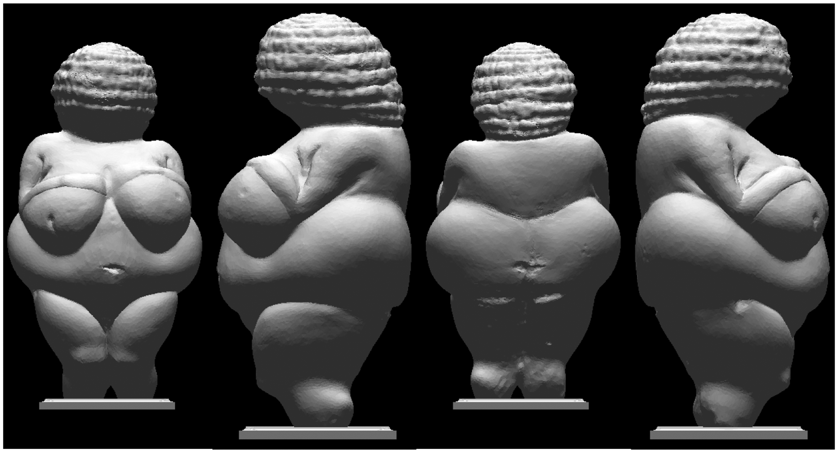

That vision prefers hills makes sense from the perspective of biology. Simple objects tend to be ovoid and to turn convexities toward the eye. Two convexities might well represent a pair instead of a single object. In such cases, it is the depth difference between the objects that counts, for that their individual reliefs are irrelevant. Suppose you see two “eggs” with one point indicated on each: What is the depth separation of the points? This question is similar to: How far is the Tour Eifel from the Brandenburger Tor? The answer is simply the distance Paris-Berlin. Their city plans are irrelevant to the question.

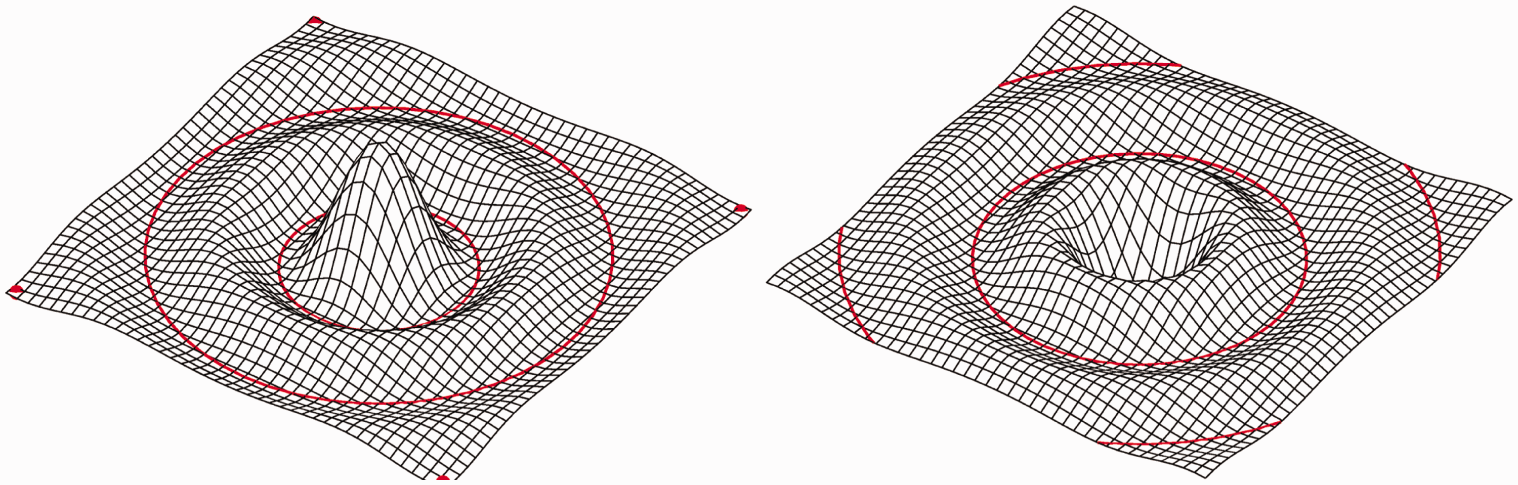
This also suggests a principled explanation of why reliefs appear so alien when their depths are inverted (Metzger, 1936; see Figure 8). In such a case hills become dales and vice versa, whereas natural dale districts are very different from natural hill districts. Thus inverted reliefs have different parts and as a consequence they elicit fully different global Gestalts (Hoffman & Richards, 1984; see Figure 9). Something similar happens when you illuminate an object from below: The dales turn into hills and the global impression cannot look normal—and, indeed, does not (Metzger, 1936)—because it has wholly unnatural parts.

Figure 8.

Example of the relief of an alpine landscape (left). At right, we show the image with the intensity scale inverted. In this negative the visually salient “parts” become very different.

Figure 9.

Two surfaces revealed through the deformations of a Cartesian coordinate mesh. The surface at right is the same as that at left except that we have inverted the vertical coordinate, thus swapping hills with dales. Notice that the visually salient “parts” become very different. (We have suggested the part-boundaries with the red curves.) Notice that this demo is similar to (but different from) that used by Hoffman and Richards (1984).

Conclusions

This study puts us in a position to answer the question posed at the introduction: Is the mental representation of pictorial relief a local or a global one? The answer appears to be that it is in-between. It is usually not global, with the exception of ovoid shapes. It is not local either, at least not in the sense of point-wise with some fixed size constraint. It is piecewise with the segmentation being similar to a distribution of “natural districts” (Maxwell, 1870). Notice that natural districts are either hills or dales and that vision singularly prefers hills. In extreme reductionistic cases concavities may be noticed, but a saddle shape (neither convex or concave), ⁵ almost never is (van Doorn, Koenderink, Todd, & Wagemans, 2012; Wagemans, van Doorn, & Koenderink, 2010).

The present study affirms a tentative conclusion from a (much) earlier experiment (Koenderink & van Doorn, 1995). In that study, we also compared point pairs with respect to depth, but using a much finer triangulation. The advantage is resolution, the disadvantage the explosive increase in the number of pairs. The number grows with the square of the number of vertices, and the number of vertices itself increases inversely with the square of the triangulation’s edge length. Thus, we used only a few fiducial vertices and compared them with all others, thus forcing only a linear increase in the number of vertices. We were able to show that the observational scatter increased when points lie on different hill slopes as compared with a single slope. The former study was necessarily flawed by the fact that observers soon became familiar with the fiducial locations. The present study does not have this problem and has still a just sufficient resolution. In any case, our previous tentative conclusion was fully confirmed.

Of course, except from answering some questions, this study suggests many directions for follow-up studies. For instance, one could try to investigate the question about the number of clusters or regions alluded to above. Moreover, the clusters are very useful in suggesting interesting fiducial points, for instance their centers of gravity. This would enable a finer grained approach if one wanted to address the perceptual organization of pictorial relief at different spatial scales. Another potentially interesting topic is the segmentation induced by the clusters. This is a segmentation that is independent of various other ways of partitioning (e.g., like that illustrated in Figure 5). How do such partitions depend upon the image structure? This is an interesting question that can now be addressed with the methods developed here. In previous experiments, we have seen that human observers even segment the interiors of silhouettes or outlines (Koenderink et al., 2012). It seems to be an important strategy of the psychogenesis of visual awareness.

In sum, the part-whole structure of pictorial relief is very basic and suggests numerous novel explorations.