Sage Journals: Discover world-class research

Abstract

The threat stemming from the use of vehicles as a weapon in urban environments may be mitigated by employing properly designed protective structures such as bollards, street furniture or landscaping options. In order to assess the performance of a barrier resistance to a vehicle impact, the initial step involves characterizing the load on the barrier. To this aim, two recently developed generic vehicle models are utilized to conduct numerical simulations of vehicle impacts on a security barrier. Various impact configurations are examined and compared based on force-time functions. In addition to comparing the impact loadings in terms of peak forces, comparisons are also done in terms of equivalent static loads, determined by computing the dynamic load factors (DLF). The study provides new insights into the characterization of vehicle impact loads on security barriers, which could improve current engineering practices in the field.

Keywords

Crash simulation security barriers vehicle impact generic vehicle models

Introduction

Vehicle security barriers preventing the entry of vehicles into pedestrian zones can effectively mitigate vehicle-ramming attacks (Figure 1). For vehicle barriers to serve as an effective mitigation solution, they must be designed, produced, and installed to protect against specific levels of threats related to vehicle category and impact velocity (Security by design (2022) and Karlos et al. (2018) provide a general methodology for protecting public spaces).

Figure 1.

Example of vehicle security barriers (VSB) commonly used in an urban environment.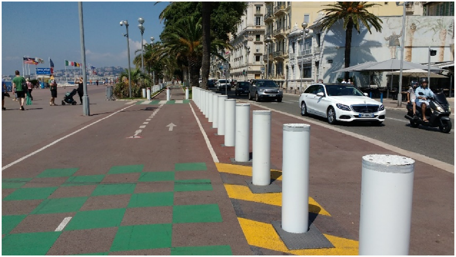

The performance of barriers against vehicle impact is certified through physical tests using real vehicles of given UNECE categories (standard ISO 22343 (2023)). Naturally, due to a relatively high cost of crash test experiments, only a limited number of tests are conducted. As a result, the information obtained from crash tests regarding barrier performance is quite limited. In particular, a crash test cannot be used to assess the safety margins of the barrier design, such as the extent to which the tested barrier could resist higher or different impact loads.

On the other hand, over the last decades, the automotive industry and research communities have acquired significant experience from the use of numerical simulations for analysing vehicle crashes, where the main objective is, in general, the passenger’s and vulnerable road users’ safety. More recently, the same type of numerical simulation tools have been introduced for analysing the performance of security barriers (e.g., Kinney et al. (2014); Hu et al. (2014); Chen et al. (2015); Ang et al. (2016); Hu (2017); Valsamos et al. (2020) and the references therein). From the perspective of numerical simulation methodology, the assessment of the performance of security barriers is very similar to the field of the bridge pier design, which needs to resist to accidental vehicle impacts Chen et al. (2018).

As in all engineering fields, the numerical simulations tools represent many advantages over the traditional engineering approaches based on experiments and simple analytical analyses. They are more accurate than the simple analytical methods and more cost efficient than physical experiments. However, when used in complex fields like crash worthiness, the use of numerical simulations in practice requires significant preliminary efforts in model verification and validation. Given the relatively scarce availability of experimental validation data in the field of security barrier performance assessment, more effort must be devoted to numerical model verification.

In general, numerical models of vehicles used for the assessment of passive safety in crash conditions are more detailed than what is needed for assessing the performance of a security barrier. Namely, the simulations of vehicle impacts on barriers do not call for representing all vehicle details (in particular for the interiors) that penalise the time required for the analysis. Since the generic vehicle models used here are developed mainly for the security barrier assessment, they represent only the vehicle properties determinant for its crash behaviour in terms of the mechanical loads transmitted to a barrier.

These models are generic in the sense that they do not represent a specific vehicle brand, but can represent most of the vehicles of a given category. This means that a generic vehicle model has to be adjustable through a set of parameters, so that its properties could fit to various configurations. In particular, with appropriate parameters can be varied the mass of the vehicle, including its distribution, the main vehicle dimensions (length, width, etc.) and some mechanical characteristics related to the crash behaviour. Two models are used for this work, one for the category N1 (small 3.5 t truck, Sebik et al. (2022)) and the other for the categories N2A and N3D (medium size trucks, from 7 t to 12 t, Sebik and Kodajkova (2023)), both being available under an open source licence JRC web page (2024).

There are two main approaches on how the numerical vehicle models can be used for the assessment of the performance of a security barrier. A full simulation approach would consist of creating a 3D model also for the barrier and run a coupled analysis of both sub-systems, the vehicle and the barrier, in the same simulation. In theory, this approach would provide the most detailed information of the performance of the barrier. In practice, it would require very detailed information not only of the barrier design itself, but also of its foundation and the surrounding soil, which might not always be easily available. The directly coupled approach is commonly used in the literature, in particular for simulating experiments (e.g., Kinney et al. (2014); Hu et al. (2014); Chen et al. (2015); Ang et al. (2016)), where all the needed information is available. A general methodology for the fully coupled methodology is described in Andrae et al. (2024), addressing also the soil-structure interaction aspects.

For situations where all the detailed information is not easily available and where only a rough assessment of the barrier performance is needed, a simpler uncoupled approach can be employed. This kind of situation is for example typical for the design process, where the vehicle impact load needs to be characterized before defining the barrier properties into details. In addition, the uncoupled approach can only be applied by considering that the barrier deforms very little during the impact and that its deformation does not influence the way the vehicle deforms during a crash. In other words, when using the uncoupled approach for assessing the dynamic loading, the barrier is considered as a perfectly rigid body. The performance of the barrier can then be assessed in a second step by applying the dynamic loading obtained in the first simulation.

The article Hu (2017) presents an exhaustive review of the simplified maximum force estimation models for the purpose of the design of bollards, the most common type of security barriers used in urban environments. The prediction of simple force estimation models is compared to some experiments and to numerous simulation results. However, the work in Hu (2017) focuses on the maximum force of the given impact scenarios and does not consider the dynamic amplification effects, due to the barrier’s elastic response. Namely, the mechanical consequences of any dynamic load depend not only on the amplitude of the imposed impact force, but also on the eigenfrequencies of the barrier system and on the frequency content of the load.

The objective of the present article is to use recently developed generic vehicle finite element (FE) models (Sebik et al. (2022) and Sebik and Kodajkova (2023)) for characterizing vehicle impact loads on a security barrier in terms of force-time functions.

Two vehicles are represented, one corresponding to the N1 category (3.5 t small size truck, Sebik et al. (2022)) and the other to the N2A category (7.2 t middle size truck, Sebik and Kodajkova (2023)), hitting a bollard in various ways. In addition to comparing the peak impact forces corresponding to different configurations, this paper proposes to analyse the impact forces also by applying a response spectrum analysis. According to this approach, a barrier system is represented as a simple mass-spring oscillator characterized by its main eigenfrequency. The response spectrum analysis is commonly used in the field of structural dynamics, in particular in earthquake engineering.

The response spectrum analysis is used here to estimate the “dynamic load factor” (DLF) of the impact force-time loadings obtained from numerical simulations using full vehicle models. The DLF applied to the peak impact force allows estimating an equivalent static load, which would lead to the same level of stresses in the barrier structure as the dynamic load itself. The simplified equivalent static approach using the DLF is very convenient for a rough and fast assessment of barrier’s performance, because it does not require a very detailed model for the barrier. As shown in this paper, the DLF strongly depends on the shape of the impact force-time function (i.e. number of peaks, their width, etc.) and on the barrier’s eigenfrequency.

The rest of the paper is organized as follows. First, the numerical generic vehicle models used for the impact simulations are briefly presented. Then the interaction of a vehicle with a barrier is discussed and the effect of the barrier natural dynamic response is evaluated. The simulation results are presented mainly in terms of the impact force-time function and discussed from the perspective of the vehicle crash behaviour, strongly dependent on the impact configuration. At the end, some conclusions are drawn, followed by recommendations for the future research work.

Generic vehicle models

It is important to stress that the aim of a generic vehicle model is not to represent any existing vehicle but to represent the whole group of vehicles of given categories defined in the standard ISO 22343 (2023). For this reason, only the features of the vehicle structure, which are brand and model independent and present (in some form) on any vehicle in its category are included in the model. Another aspect, which governs the decision, which parts of the vehicle should be included and which should be omitted, is the requirement for the computational efficiency of a simulation.

The vehicle models considered here are designed specifically for virtual barrier testing. Unlike typical vehicle models used for passive safety assessment, they do not need to represent components that have negligible impact on crash behaviour. As a result, the model includes only the components that are crucial for crash stiffness and vehicle mass distribution, ensuring the vehicle model can accurately simulate the impact on the barrier. In addition, the crash effects of parts, which do not (or very little) contribute to the overall behaviour of the vehicle impact behaviour like dashboard, seats, components of passive safety and similar are unimportant for these analyses and they do not need to be represented in the model. However, in the used models the total mass is preserved by increasing the mass of other modelled components.

To limit the change in the crash behaviour, any additional mass added to compensate for omitted components can only be applied to non-deforming components during impact.

Following this approach two different generic vehicle models have been created recently, one for the category N1 Sebik et al. (2022) and one for the categories N2A and N3D Sebik and Kodajkova (2023). Since the variations of the general vehicle architecture between the vehicles on the market for the categories N2A and N3D are not very significant, one single model can cover both categories. The N1 category is more specific and is treated apart. Both models are illustrated in the Figure 2.

Figure 2.

Finite element meshes of the generic vehicle models for the N1 category (3.5 t small truck, on the left) and for the categories N2A and N3D (from 7t to 12t medium size trucks, on the right).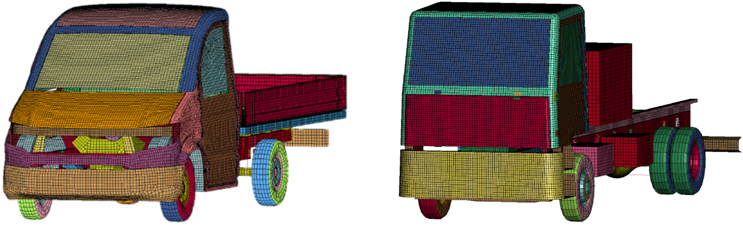

The finite element models (Figure 2) were created with LS-Dyna software and are mainly composed of shell elements. Additionally, solid elements are used for the massive components (e.g., engine and gearbox), as well as some beam elements, but to a lesser extent. The N1 model contains approximately 80,000 elements, while the N2A/N3D model contains about 180,000 elements. The element size varies between 10 mm and 50 mm and the critical time step is about 3 μs (0.003 ms), which makes the model computationally cost efficient. Altogether, the models require only a couple of hours CPU time for typical impacts simulations (100–500 ms) using a common laptop computer.

Figure 3.

Bottom view pf the generic vehicle model for categories N2/N3. Two main components in terms of the crash behaviour, the frame and the engine, are highlighted.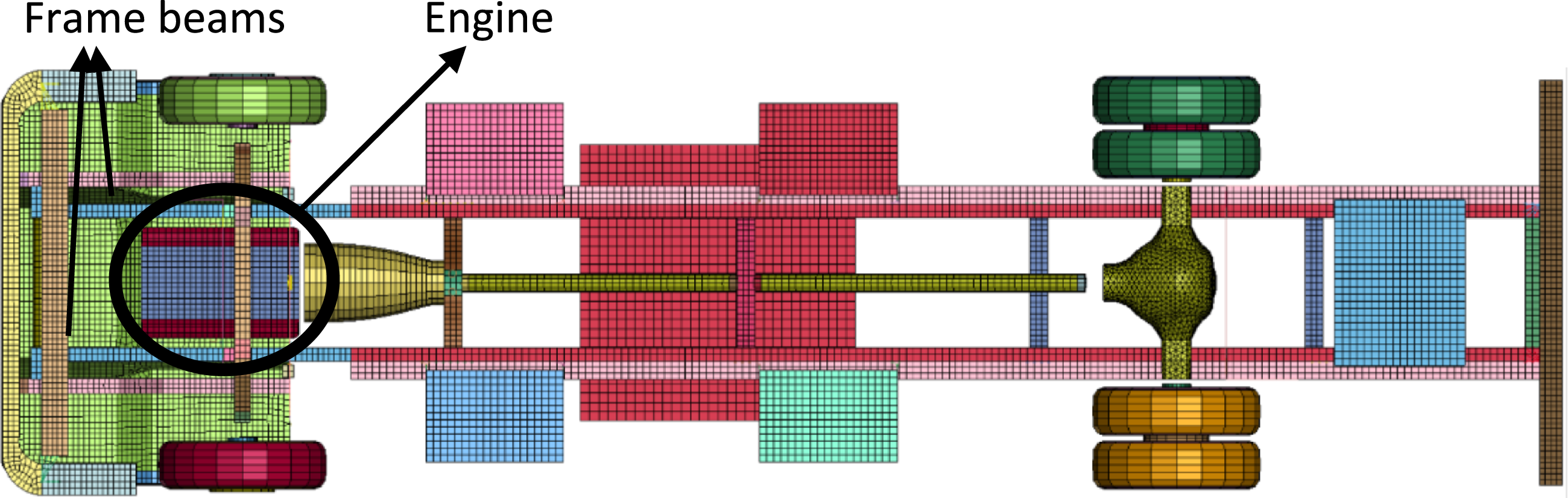

The above-mentioned models have been validated following the standard CEN/TR 16,303 and through comparisons to various crash tests. The N1 generic model was validated by simulating two crash scenarios: one with a Ford Ecoline 56 km/h crash on a rigid wall Sebik et al. (2022) and the other with a 3.5 t vehicle 48 km/h crash on a bollard Saraceno (2023). As for the N2A/N3D model, it was validated by comparison to three crash tests of 7.5 t trucks, two at 48 km/h (Sebik and Kodajkova (2023) and Spizzirri (2023)) and one at 80 km/h Ravedati (2023). The comparisons between the simulations and experiments are based on the values of displacements, velocities and accelerations of different points on the vehicle during the impact.

Barrier load characterization

Vehicle crashing behaviour

A vehicle ramming threat is usually defined only by the vehicle category, its total mass and the impact velocity. However, the actual load on a barrier also depends on the mass distribution, the stiffness of different vehicle components, and the connections between these components. The most important component for the crash behaviour is the frame (i.e., the chassis), composed of two frame beams, connected with several cross-members and to which all other components are connected directly or indirectly (Figure 3). During an impact on a rigid barrier, the frame absorbs the largest part of the total energy. Its overall crushing mechanism and strength directly determine the impact duration and, consequently, the average impact force. The stiffer the frame, the shorter will be the impact duration and the higher the average force for the same initial vehicle velocity.

Figure 4.

The barrier is considered as a simple spring-mass system in order to estimate the phenomenon of the dynamic amplification due to barrier elasticity.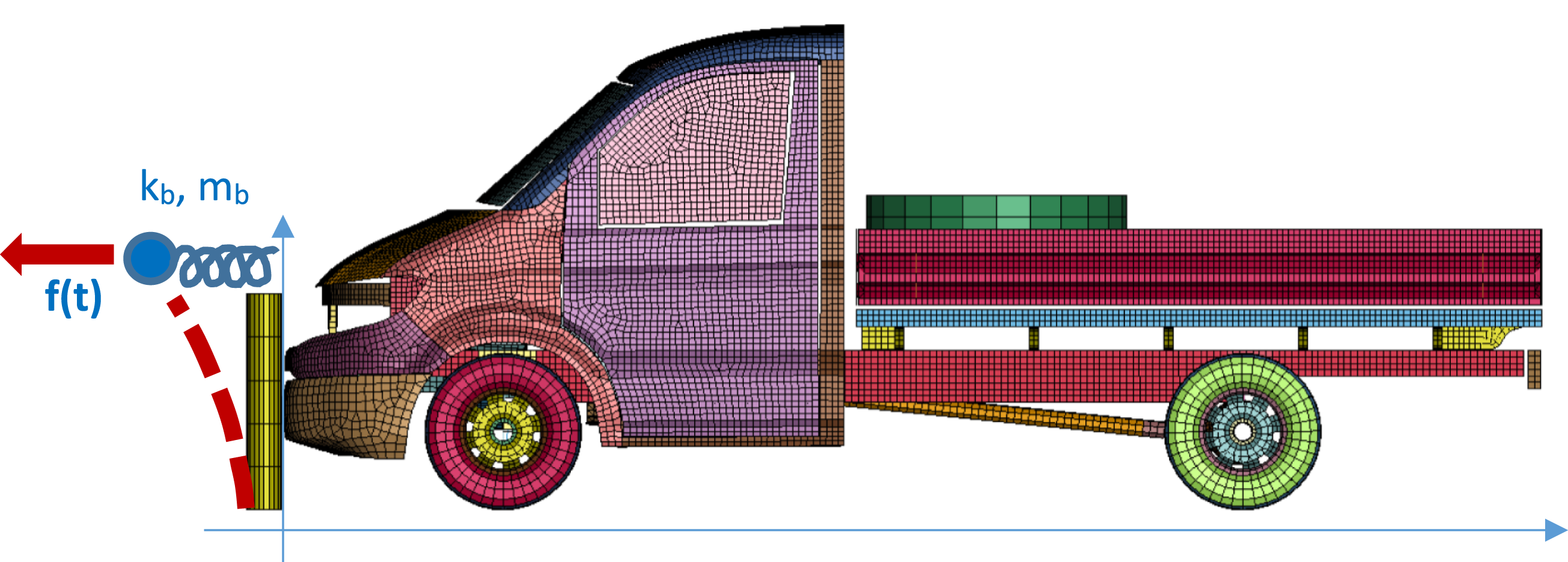

In addition, the force peaks depend much more on other components, in particular on the engine (Figure 3), which is a relatively big, heavy and rigid component, and in this sense very different from all other components. In typical configurations (e.g., Chen et al. (2015) or Chen et al. (2018)), the engine is responsible for the highest force peak acting to the barrier. The amplitude and the length of the peak corresponding to the engine hitting the barrier depends also on the connection with the frame. Even if the engine itself can be considered as very rigid, in reality it is surrounded with smaller components typically not represented in the model (e.g., cables, tubes) which are flexible and have a certain shock absorption capacity, difficult to quantify in practice. Therefore, in Sebik et al. (2022) and Sebik and Kodajkova (2023) the very stiff engine model is adjusted so that it has an additional softer layer representing the non-modelled components. The material properties of this artificial additional layer were calibrated in a way that the simulation results would match best the analysed crash experiments.

The vehicle crashing behaviour is strongly dependent on the type and the characteristics of the barrier. This is true also for the rigid, little deforming barriers. In particular, the shape of a barrier is determinant for the contact surface with the vehicle. For instance, if the contact surface is smaller (i.e., the load is more concentrated), the total impact force should decrease. Therefore, since the total impulse must be equal to the initial vehicle momentum, the duration of the impact is elongated and the average force decreases.

Analytical estimations for the impact force

Analytical methods for estimating the impact force from a vehicle crash have mainly been developed for designing road structures (e.g., bridge columns) against accidental vehicle ramming. Nevertheless, there is no difference between accidental and malicious vehicle ramming in terms of impact load estimation. An exhaustive review of existing formulas for maximum impact force assessment is provided in Hu (2017), where various methods are evaluated by comparing them with experimental and numerical simulation results. The review Hu (2017) confirms that the “Eurocode 1: Part 1-7” (EC1) provides a relatively good estimate of the maximum force from vehicle impact. According to Hu (2017) some other analytical methods perform better but require more input parameters. Specifically, the formula from the EC1 (2006)

f_{i m p} = v \cdot \sqrt{k m}

needs as a specific input only the vehicle equivalent stiffness, k, while v and m are the vehicle impact velocity and mass, respectively. The review paper Hu (2017) considers a value k = 1200 kN/m to be appropriate, even though reference EC1 (2006) suggests using k = 300 kN/m for the equivalent vehicle stiffness. Neither of these references clearly indicate to which vehicle categories the equivalent stiffness values should apply, even though the value of k is expected to strongly depend on the type of the vehicle. In any case, since the value of k cannot be determined with accuracy, precautions should be taken when using this simple impact-force characterization approach.

In addition, it is important to stress that according to EC1 (2006) the duration of the impact force, ∆t, is

∆ t = \sqrt{\frac{m}{k}}

which guarantees that the impact force impulse equals the initial vehicle momentum:

f_{i m p} \cdot ∆ t = m \cdot v .

in the case of dynamic loading, the stress levels experienced by the impacted structure depend not only on the load function but also on its dynamic properties. To estimate an “equivalent static force” that replicates the same maximum stress levels as the original dynamic loading, the peak impact force needs to be multiplied by the “dynamic load factor” (DLF):

f_{e q} = {D L F \cdot f}_{i m p}

For the impact load function proposed by EC1 (2006), the dynamic amplification would be always equal to two (DLF = 2), since the normal periods of structures of interest here (i.e., security barriers) are expected to be smaller than the duration of the load, Δt.

It is important to stress that the analytical estimations for impact force, such as those presented in the EC1, assume a simple rectangular impulse load function. This assumption allows for straightforward calculations using standard dynamic or even static analysis approaches. However, in reality, impact loads are typically more complex, exhibiting a time-varying nature that may have several peaks, as shown later in this paper.

Computation of the force-time loading function

In the impact simulation, the vehicle and the barrier interact through contact (i.e., non-penetration) condition and the interaction force, which represents the load on the barrier and is equivalent to these contact forces.

In general, there are two families of numerical algorithms, which can be used to impose a non-penetration (i.e., contact) kinematic condition: the method of Lagrange multipliers and the so-called penalty method (e.g., Wriggers (2006)). In the Lagrange multiplier method, the contact forces are computed such that the desired non-penetration condition is satisfied exactly. Whereas in the penalty method, the kinematic constraint is satisfied by introducing an additional stiffness at the contact surfaces such that it prevents significant inter-penetration between the two bodies.

The main inconvenience of the penalty method is that it introduces additional stiffness parameters difficult to define without a trial-and-error approach. On one hand, if the contact stiffness is too small, there will be an unacceptable penetration between the interacting bodies (i.e. vehicle and barrier). On the other hand, if the stiffness parameter is too big, this will penalize the critical time step and the computation can become prohibitively long. However, there seem to be no sound theoretical approaches for selecting the stiffness parameters effectively for any practical situation (e.g., Gonzales et al. (2021)). Therefore, the appropriate stiffness parameters need to be selected on a case-by-case basis. Nevertheless, the penalty approach is often preferred in crash analyses, because it is considered as more computationally effective than the Lagrange multipliers method, which requires a more complex solving algorithm, in particular for parallel simulations.

In both cases, the computed contact forces result from the non-penetration kinematic condition and do not necessarily correspond to realistic physical forces. Namely, the numerical contact forces have a clear physical meaning only in terms of the impulse they create during the contact interaction between the two bodies. Therefore, if the time step is changed when using the Lagrange multiplier method, the contact forces will be adapted so that the impulse (force multiplied by the time step) would remain the same. Regarding the penalty method, the contact forces are strongly dependent on the stiffness parameters used.

Thus, the contact forces computed directly by the simulation software, whatever algorithm used, are not perfectly representative of the loading forces of the barrier. Typically, the force history corresponding to the contact obtained by the simulation software contains a significant high frequency numerical noise. Therefore, in the standard engineering practice, a low pass filter is applied to the contact force outputs, wherever the contact force values are needed (e.g., Chen et al. (2018)). According to the common practice, the force-time output functions are filtered using the “Society of Automotive Engineers (SAE) Class 60 Filter” Warrendale (1995).

The contact-impact algorithms respect, by construction, the conservation of the momentum. Hence, an alternative way to compute the impact forces is to apply a numerical derivation scheme to the momentum-time function computed by the simulation software. In this case, instead of frequency based filtering, the calculated forces are filtered by choosing the time-step for the numerical derivation. In fact, both procedures introduce a numerical artefact, but the physical meaning of the derivation time-step seems more straightforward to interpret than for the low-pass filtering approach, developed initially for general signal processing, not specifically for mechanical systems.

We have also observed that sometimes the force-time functions exported from a simulation software by using the filtering approach mentioned above do not conserve the total momentum, i.e. their integrals are sometimes non-negligibly smaller than the initial momentum.

Therefore, in the numerical examples presented here and for the above-mentioned reasons, the force-time functions were obtained by the numerical derivation of the momentum-time functions calculated by the software instead of using the filtered force-time functions.

Barrier response

The barrier dynamic response depends not only on its design (dimensions, materials, etc.), but also on its interaction with the environment through its foundation, which can be of very different types (shallow, deep, etc.). Simulating the entire system barrier-foundation-environment is feasible, but requires a lot of input information, in addition to being computationally costly Andrae et al. (2024).

In order to obtain a conservative estimation of a vehicle impact load, it is convenient to assume that the barrier undergoes a very small deformation, not affecting the crashing behaviour of the vehicle. Under this assumption, the impact force-time load is independent from the barrier’s dynamic response and can be computed by a simulation assuming a completely rigid barrier.

When using a force-time function to assess the response of the barrier it must be assumed that the contact surface does not change significantly during the impact. Otherwise, the uncoupled approach would not be appropriate.

The assessment of the barrier response to the impact can be done by using similar simulation tools as the ones used for vehicle crash analyses. In addition, it is possible to use the so-called “equivalent static force” approach, according to which a static force is determined to induce the same maximum deformation of the barrier as the direct dynamic analysis approach.

Figure 5.

Bollard geometry used in the simulations, considered as perfectly rigid.

In order to estimate the effect of the elasticity of the barrier on its dynamic response, it is represented by a one degree of freedom simple elastic oscillator (Figure 4). Then, the dynamic response of the barrier satisfies the following simple equation:

m_{B} \ddot{u} + k_{B} u = f_{v e h} (t),

(1)

where m_B and k_B are the barrier’s effective mass and stiffness, respectively, and f_veh(t) is the force-time function obtained by the vehicle impact simulation in which the barrier is considered as perfectly rigid.

Figure 6.

N1 vehicle finite element model.

For the discussed purposes, the spring-mass can be sufficiently characterized by its natural angular frequency, corresponding to

ω^{2} = \frac{k_{B}}{m_{B}} .

Actually, the effective mass and stiffness, m_B and k_B, do not really need to be specified explicitly. By using the following transformation:

w (t) = k_{B} u (t),

the above dynamic equation (1) becomes:

\ddot{w} + ω^{2} w = ω^{2} f_{v e h} (t),

(2)

The introduced variable w is the internal force corresponding to the barrier’s deformation state defined by u. It is important to stress that none of the variables u and w have a straightforward physical interpretation. Nevertheless, the maximum value of the variable w must correspond to the most deformed barrier configuration and the “equivalent static force” can be computed as:

f_{e q} (ω) = \max_{t} (w_{ω} (t)) .

In practice, the equation (2) for the given force-time function, f_veh(t), is solved for the set of N barrier frequencies of interest

ω_{i}

, i = 1,2,...N. There are several possibilities for solving the simple scalar equation (2). In this work, the standard central difference time integration scheme was used, most common for impact simulations in general.

Then the “equivalent static force” is obtained for each barrier natural frequency of interest, $ω_{i}$ , by finding the maximum value of the corresponding w time history. In addition, the “dynamic load factor” can be determined as:

D L F (ω) = \frac{f_{e q} (ω)}{f_{i m p}},

where f_imp is the peak value of the force-time function (Section “Analytical estimations for the impact force”)

{f_{i m p} = \max}_{t} (f_{v e h} (t))

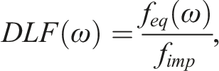
It is important to stress that the DLF is a non-trivial function of $ω$ which depends strongly on the shape of the force-time function f_veh(t). In fact, only the extreme limit values do not depend on the shape of the force-time function, i.e., $D L F \overset{ω \to 0}{\to} 0$ and $D L F \overset{ω \to \infty}{\to} 1$ . Both these limits follow directly from equation (2) and have a direct physical meaning. When the barrier has a very long normal period ( $ω \to 0$ ), any load has a negligible short duration and the barrier’s response is null. On the other hand, when a barrier is very stiff ( $ω \to \infty$ ), any load acts like if it was static.

For any other (finite) value of $ω$ , there is no general upper limit for the value of the DLF. Such a bound exists only for simple force-time functions with at most one peak (e.g. triangular or step functions, see Biggs (1964)), for which DLF ≤2. However, for time functions with several peaks, this upper bound does not hold and the DLF can exceed a value of two, as is shown in the next section. As higher DLF are somehow associated to resonance effects, typical for quasi-stationary oscillations, they depend very much on the proximity between the barrier’s natural frequency and the characteristic frequencies of the force-time function.

Although the “equivalent static force” approach is much less accurate than the fully coupled simulation approach, especially for barrier systems expected to undergo multimodal dynamic responses or non-linear deformations, it is more practical for rapid assessment and can help in selecting the most critical vehicle impact scenarios for a given barrier.

Additionally, it is important to note that using the perfect rigidity assumption to determine the force history for flexible barriers overestimates the force amplitude Valsamos et al. (2020), ensuring the conservatism of the approach.

Numerical results

The objective of the presented numerical simulations is to assess the sensitivity of the impact load on a rigid barrier of different crash configurations. Two different vehicle models are used (Section “Generic vehicle models”) for impact simulations on a rigid bollard (Figure 5) with common characteristics. In all simulations, the considered impact velocity was set to 48 km/h. All the simulations were performed in the framework of three master thesis projects (Spizzirri (2023), Ravedati (2023) and Saraceno (2023)).

For each category of vehicles, N1 and N2A, several simulations were conducted by varying only the vehicle position with respect to the bollard. As it is shown further on, the relative vehicle-bollard position changes significantly the crashing stiffness of the vehicle reflected by significantly different force-time functions, even if the initial vehicle velocity and mass are kept the same.

In the following, the results are first presented individually for each vehicle category and then compared. Regarding the finite element meshes, for the vehicles models were used element sizes based on past experience and are in the range from 11 mm to 50 mm. The mesh is finer for the front components undergoing large deformations during an impact and coarser for the components less deformed during an impact.

Since in the simulation the bollard is modelled as rigid, the mesh elements cannot deform and can be relatively big, but only in the vertical direction (∼200 mm), because in the circumferential direction (∼20 mm) they need to accurately represent the circular shape. The bollard mesh element size could influence the simulation results only through the impact-contact algorithms, which can be sensitive to the element size differences between two objects in contact. However, no particular numerical issues were encountered in the simulations.

Results for the vehicle of N1 category

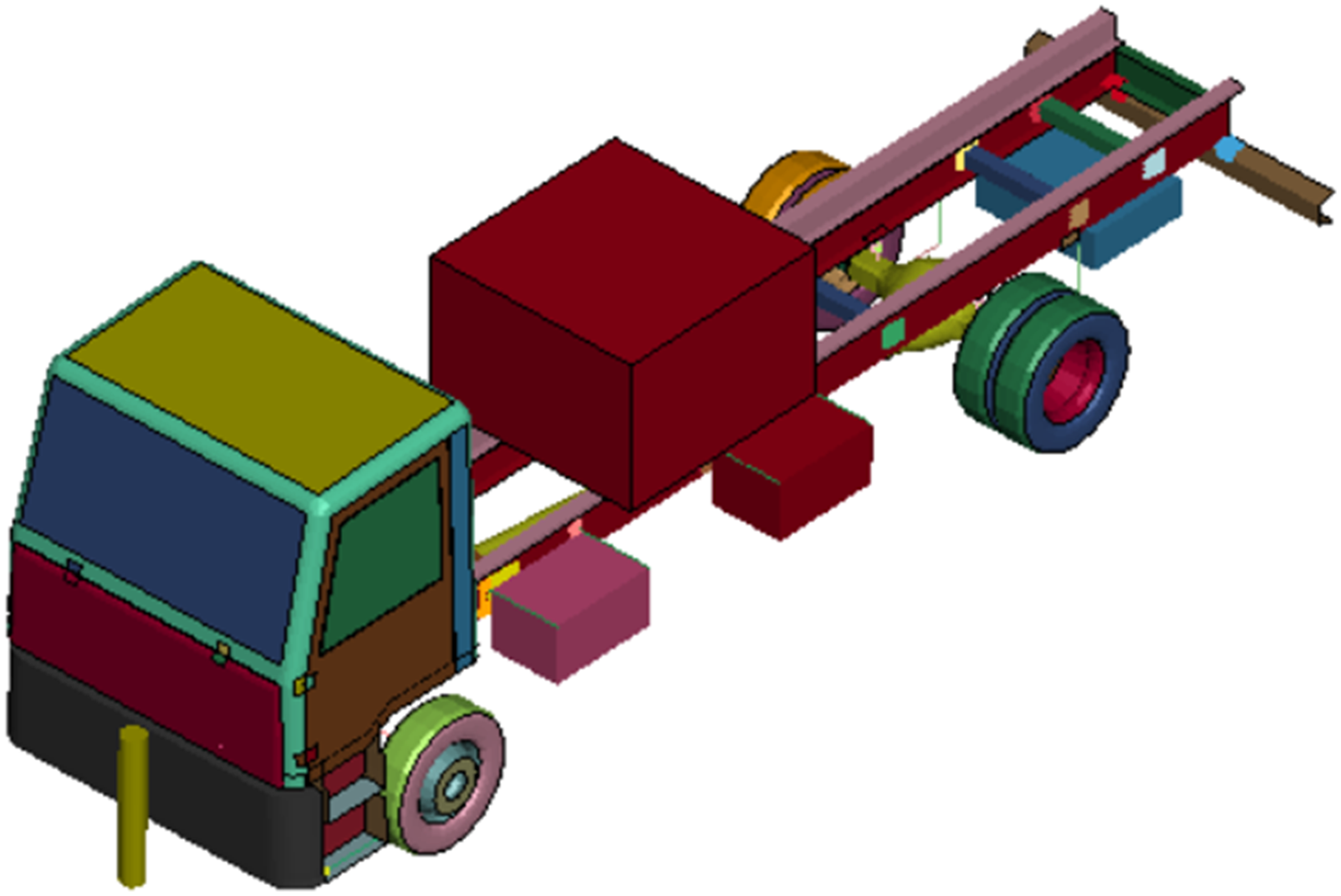
The N1 category corresponds to a family of small trucks, with maximum mass of 3.5 t ISO 22343 (2023). The basic characteristics of the model used are the following:

• Wheelbase (horizontal distance between the front and rear wheels): 3420 mm

• Vehicle length: 5820 mm

• Total mass (vehicle, including cargo): 3500 kg

All the details of the N1 model (Figure 6) are available in the report Sebik et al. (2022).

Figure 7.

N1 vehicle model in the position of hitting the bollard in the centre (view from above).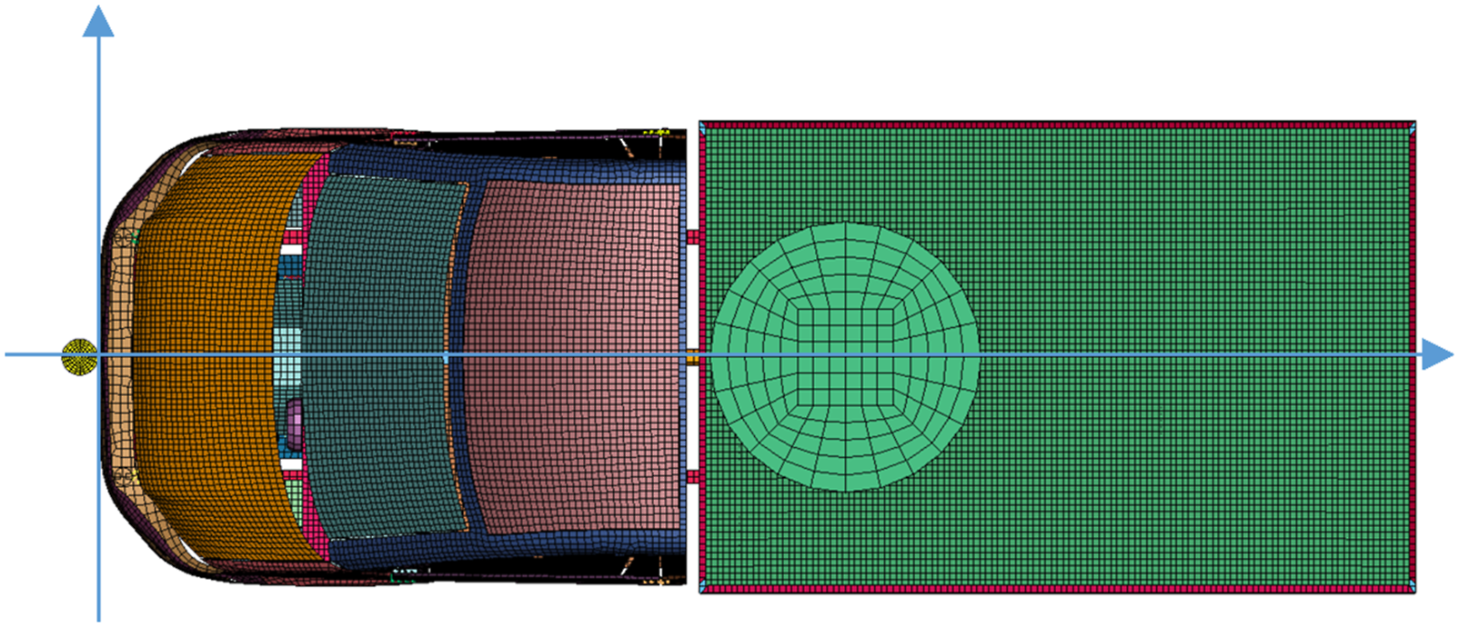

The baseline simulation considers an impact of the bollard with the exact centre of the vehicle with respect to the traversal direction (Figure 7). This is the most typical testing configuration and was also used for the validation of the model Sebik et al. (2022).

Figure 8.

Force-time function obtained from the vehicle impact on a rigid bollard with the N1 model (top figure) and extractions from the impact simulation with the N1 model (bottom view) at different instants (three bottom figures). The image (a) corresponds to the instant when the engine hits the bollard (shown in dark yellow), producing the highest force peak. After this shock, the engine rebounds (b) and hits the bollard again (c) with a smaller velocity.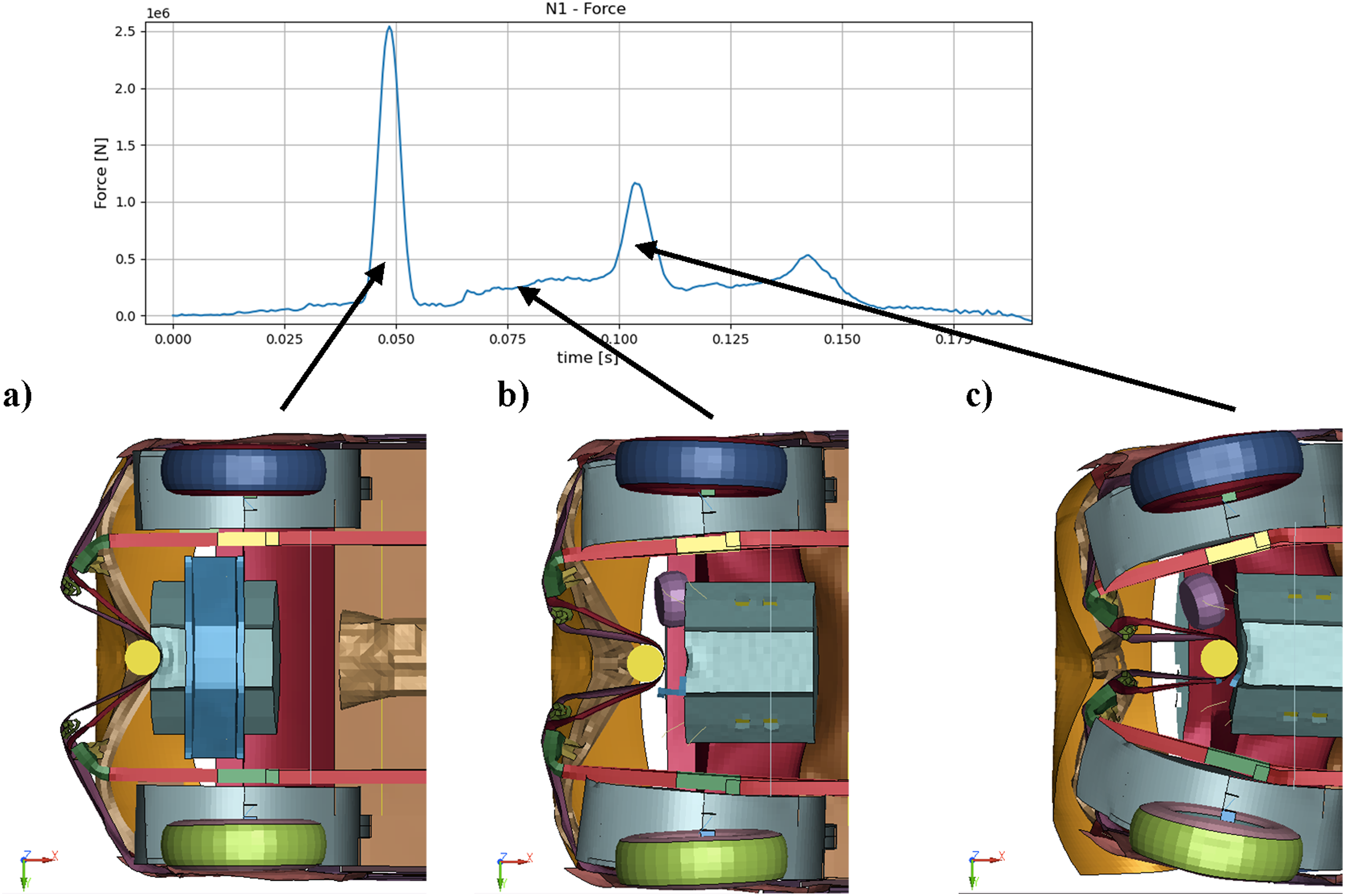

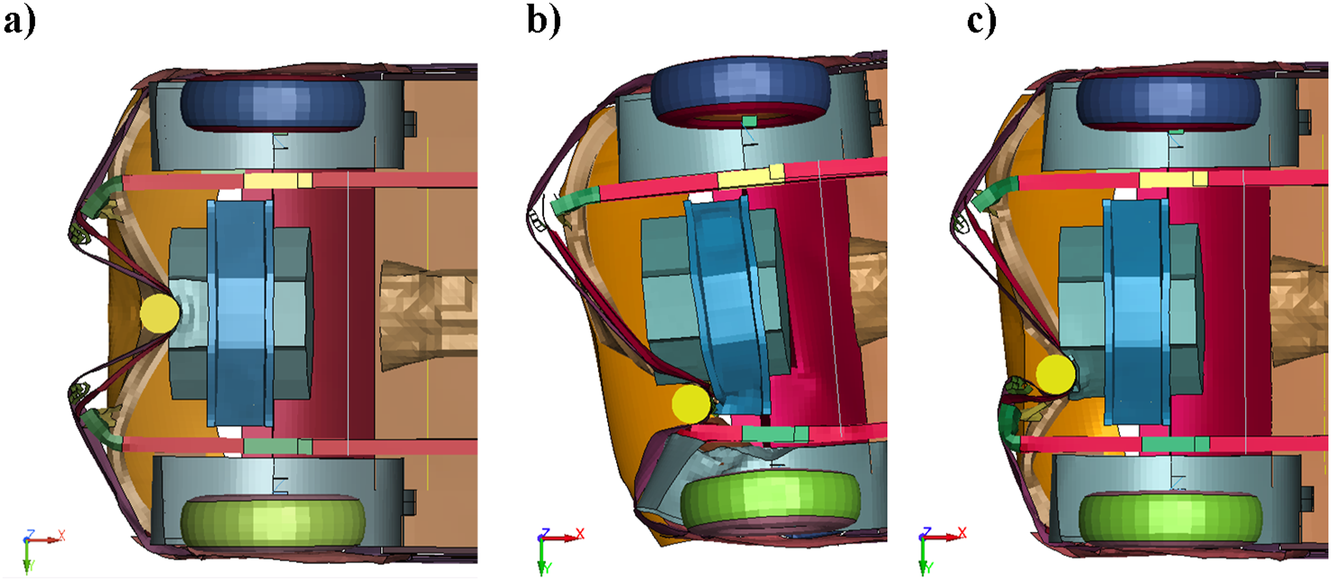
The corresponding force-time function is presented in Figure 8. The main load duration is about 170 ms and is mainly characterized by three peaks. From the analysis of vehicle deformation plots it results that all the force peaks correspond to the instants when the engine interacts with the bollard. Since the front part of the vehicle is relatively flexible, designed to absorb part of the impact energy, the impact force as well as the vehicle deceleration are low in the beginning of the crash. Therefore, when the stiff engine comes into contact with the bollard, its velocity has not decreased a lot and the force of the shock is close to the initial vehicle velocity (Figure 8, image a). The engine deforming almost elastically, it rebounds from the bollard and starts moving in the opposite direction with respect to the impact (Figure 8, image b). After some additional 50 ms, the engine hits the bollard again and produces the second force peak (Figure 8, image c). The engine rebounds and impacts the bollard for a third time, but with a much smaller amplitude.

Figure 9.

Alternative impact scenarios. Instead of hitting the bollard with its centre (Figure 7), in the two configurations above, the bollard is shifted to one side and the impact is not symmetric. In the configuration of the bottom image, the vehicle hits the bollard straight with one of the frame beams. On the left hand side the full vehicle impact configurations, on the right hand side a detailed view of the vehicle frame and engine respect to the bollard.

Figure 10.

Vehicle-bollard interaction modes for different impact configurations (the bollard is shown in dark yellow): centred (a), aligned with the frame beam (b) and intermediate (c). In contrast to configurations (a) and (c), where the engine hits the bollard directly, in configuration (b), the bollard is first impacted by the frame beam and then by the frame cross member, but never directly by the engine.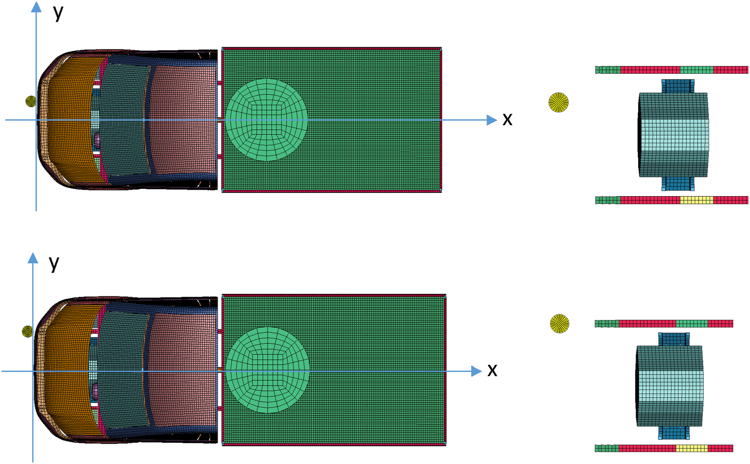

In addition to the central impact, two alternative configurations have been analysed (Figure 9). One corresponds to the case where one of the frame beams would be aligned with the bollard. As the frame is the key component of the vehicle, it is expected that the impact would be stiffer than for the centred configuration, at least in the beginning of the impact. A third configuration is added, in which the vehicle hits the bollard in the middle between the frame beam and the centre.

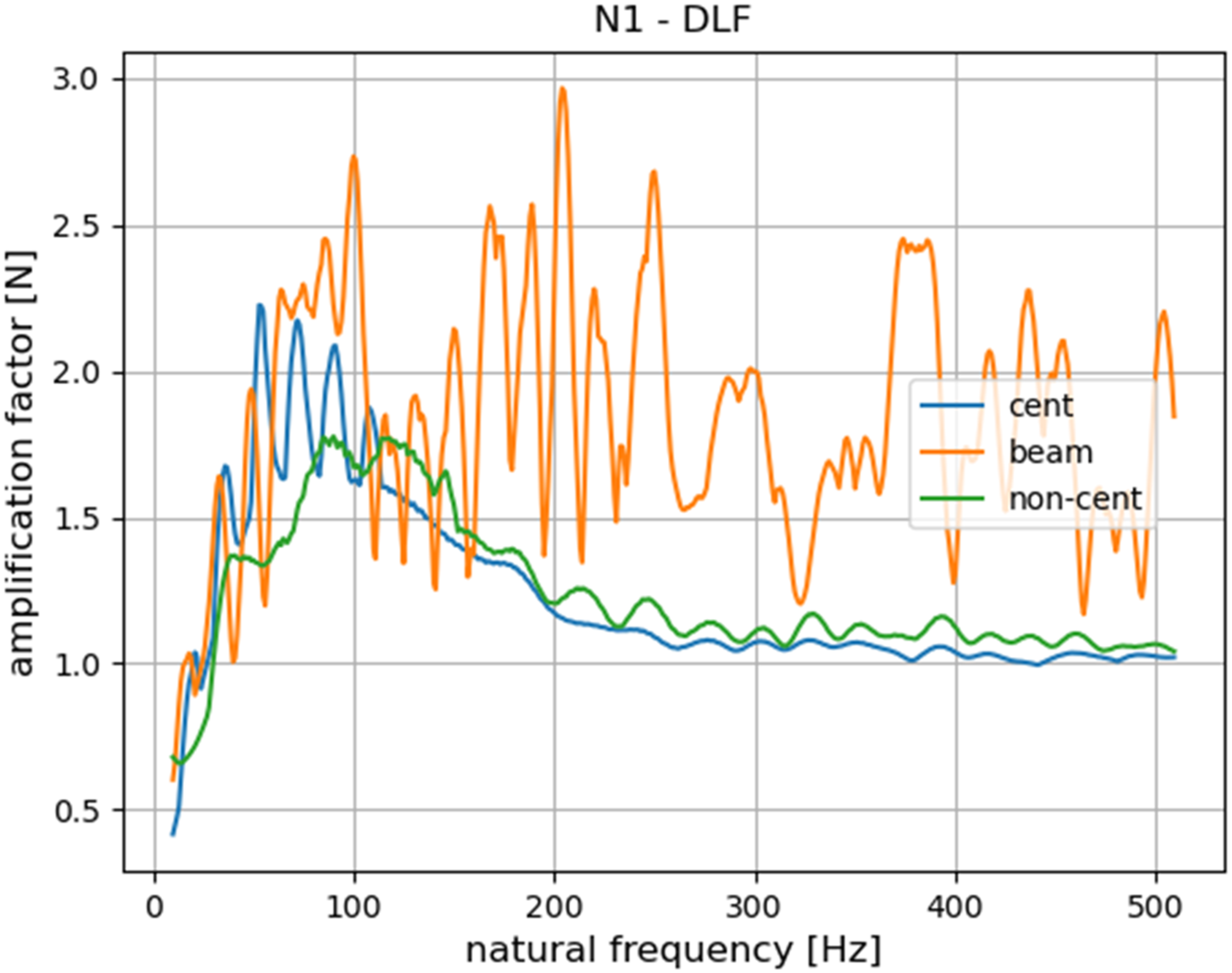
The way the vehicle interacts with the bollard during the impact varies a lot between the three different configurations (Figure 10), which is also reflected in the force-time diagrams (Figure 11).

Figure 11.

The momentum-time plot (on the left) and the force-time plot (on the right) for the N1 simulations for the three different impact configurations: centred, frame beam-centred and non-centred.

Figure 12.

The “dynamic load factor” (DLF) depending on the natural frequency of the barrier system for the N1 simulations for the three different impact configurations: centred, frame beam-centred and non-centred.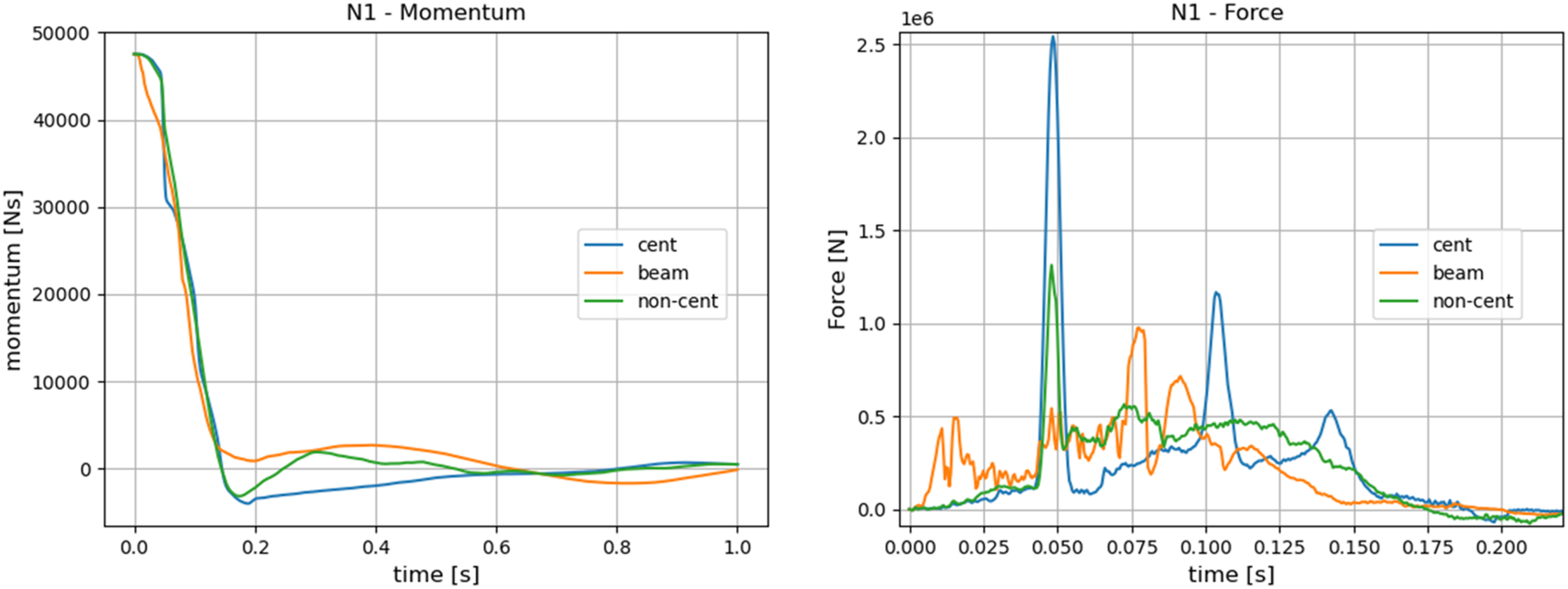

The momentum-time plot (Figure 11) allows to assess when the vehicle comes to a stop. In this context, “momentum” corresponds to the vehicle’s momentum, which is the sum of the product of the node velocity and the nodal mass over all vehicle finite element mesh nodes. For the “centred” and “non-centred” scenarios, the impact ends at around 170 ms, whereas for the “beam-centred” scenario the momentum reaches a plateau close to zero at around 150 ms. It is important to stress that here only the behaviour in the main direction (longitudinal, along the initial vehicle velocity) is analysed, but the vehicle response is fully 3D. In particular, in all scenarios a vertical displacement of the rear part of the vehicle and some rotation around the vertical axes for the non-symmetric scenarios (“beam-centred” and “non-centred”) are observed. One of the consequences of this complex vehicle behaviour is that it is practically impossible to determine the impact duration with accuracy.

In the force-time diagram (Figure 11), it is possible to observe that the “beam-centred” scenario leads to higher forces in the beginning of the impact, since the frame beam is much stiffer than the front bumper and its cross members components. Nevertheless, the “centred” and “non-centred” scenarios lead to much higher force peaks, because in these cases the engine impacts the bollard directly, which is not the case for the “beam-centred” scenario. In addition, the engine shock is much stronger for the “centred” scenario than for the “non-centred” one.

In any case, as already stressed in the Section “Computation of the force-time loading function”, the maximum force is not completely determinant for the stresses supported by the barrier system. Namely, as for a dynamic loading in general, the consequence of an impact load, in terms of maximum stresses in the barrier, does not only depend on the peak value of the force-time function, but also on how it interacts with the natural dynamic response of the barrier system. Since here the duration of the impact load is much larger than the expected natural periods, the barrier response can be amplified due to resonance effects.

Figure 12 presents the “dynamic load factors” (DLF) depending on the barrier’s natural frequency (defined in the section “Computation of the force-time loading function”) for the three configurations considered above. The “equivalent static load” is presented in the Figure 13. It is important to stress that the “equivalent static load” graph is equal to the DLF graph scaled by the force peak value. Therefore, even if the DLF of the “beam-centred” scenario is globally bigger than the DLF of the “centred” scenario, the corresponding “equivalent static force” is much higher for the “centred” scenario because of the much higher peak force.

Figure 13.

The “equivalent static force” depending on the natural frequency of the barrier system for the N1 simulations for the three different impact configurations: centred, frame beam-centred and non-centred.

Figure 14.

Finite element model of the N2A vehicle.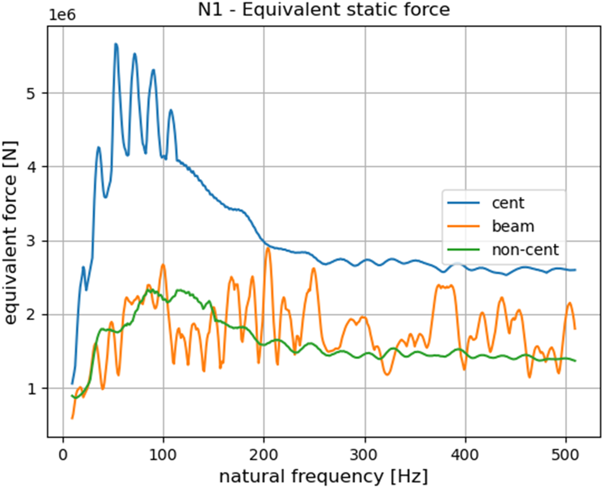

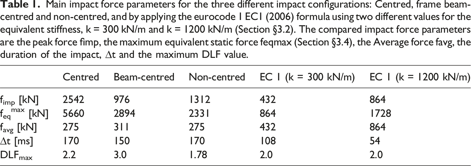
Table 1 compares the simulation results in terms of the peak impact force, f_imp, and the equivalent static force f_eq^max (Section “Barrier response”) with the impact force parameters obtained with “Eurocode 1: Part 1-7” EC1 (2006) formulas (Section “Analytical estimations for the impact force”). Additionally, the values of the impact duration, ∆t, and the average impact force, f_avg are also compared. It is important to stress that while for the EC1 approach the value for ∆t is given directly (§3.2), in the numerical simulation it is difficult to determine when exactly the vehicle comes to stop, due to significant oscillations of the force-time function.

Table 1.

Main impact force parameters for the three different impact configurations: Centred, frame beam-centred and non-centred, and by applying the eurocode 1 EC1 (2006) formula using two different values for the equivalent stiffness, k = 300 kN/m and k = 1200 kN/m (Section §3.2). The compared impact force parameters are the peak force fimp, the maximum equivalent static force feqmax (Section §3.4), the Average force favg, the duration of the impact, ∆t and the maximum DLF value.

	Centred	Beam-centred	Non-centred	EC 1 (k = 300 kN/m)	EC 1 (k = 1200 kN/m)
f_imp [kN]	2542	976	1312	432	864
f_eq^max [kN]	5660	2894	2331	864	1728
f_avg [kN]	275	311	275	432	864
∆t [ms]	170	150	170	108	54
DLF_max	2.2	3.0	1.78	2.0	2.0

The estimation of the impact duration can lead to a direct determination of the average impact force: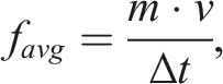

f_{a v g} = \frac{m \cdot v}{∆ t},

where m and v are the vehicle mass and impact velocity, respectively. Since these are independent of the considered configurations, the estimation of the average impact force depends only on the estimation of the impact duration. It is important to stress that for the analytical EC1 approach:

f_{a v g} = f_{i m p}

since by construction the impact force is constant over a given time interval and the maximum and average forces are equal. In addition, for the EC1 approach DLF = 2 always holds, as it applies to rectangular force-time functions with a sufficiently long duration (Biggs (1964)).

Results for the vehicle of N2A category

The N2A category corresponds to a family of medium heavy trucks, with maximum mass of 7.2 t ISO 22343 (2023). The basic characteristics of the model used are the following:

• Wheelbase (horizontal distance between the front and rear wheels): 5090 mm

• Vehicle length: 8500 mm

• Total mass (vehicle, including cargo): 7200 kg

Other details on the N2A model (Figure 14) are available in the report Sebik and Kodajkova (2023).

Figure 15.

Four impact scenarios analysed with the N2A model. In addition to the three scenarios considered with the N1 model (“centred”, “beam-centred” and “non-centred”), a fourth scenario is considered, according to which the vehicle hits the bollard a bit further away from the centre than the frame beam. The considered bollard distances from the vehicle symmetric axe are: 0 mm (“centred”), 150 mm, 400 mm (“beamcentred”) and 750mm (“outlying”). On the top, the whole model from above is shown and in the bottom the vehicle without the cabin.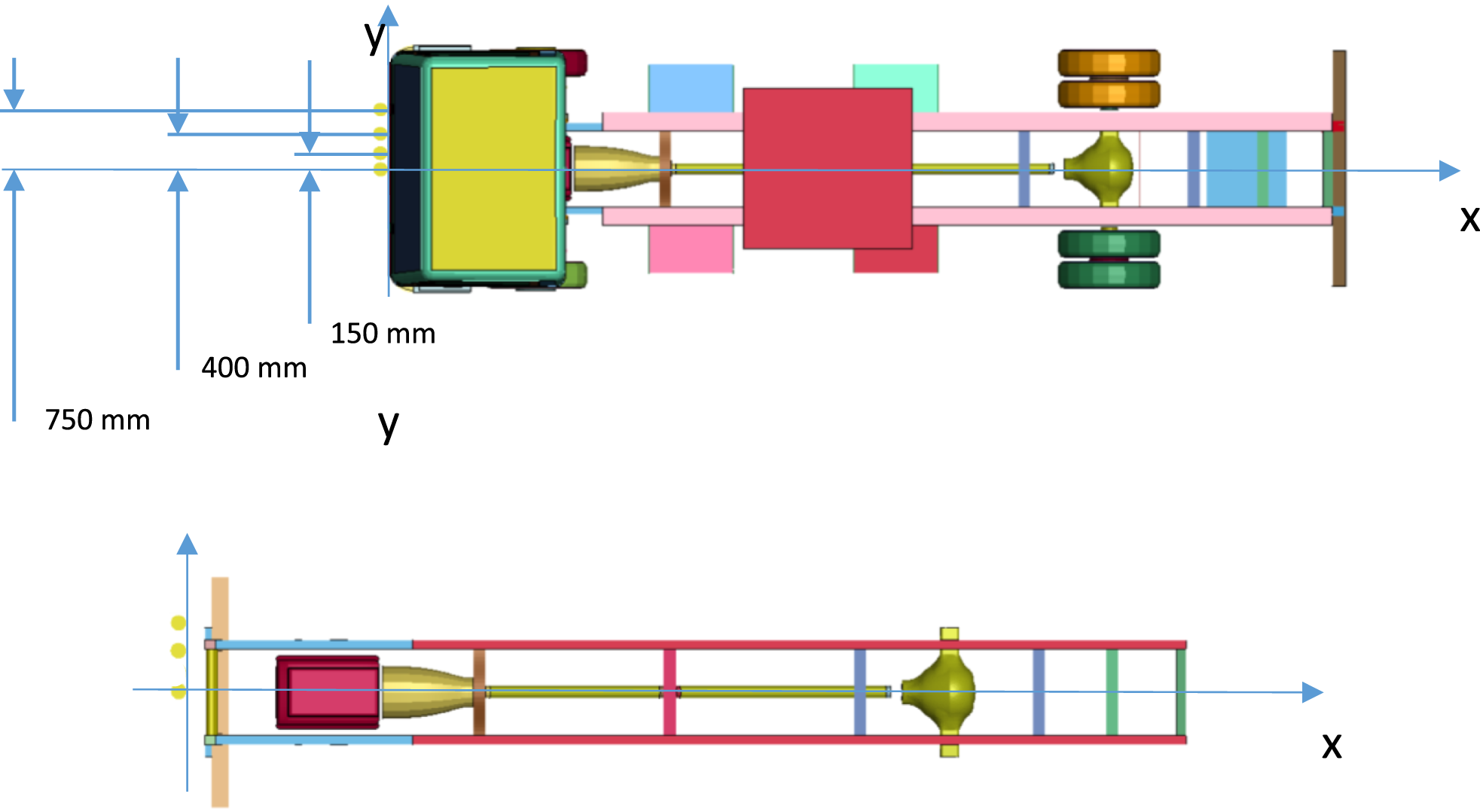

Similarly to the simulations performed with the N1 model (Section “Results for the vehicle of N1 category”), several relative bollard-vehicle positions were analysed. In addition to the baseline “centred” scenario, there were also considered positions where the bollard-to-vehicle centre distance is equal to: 150 mm, 400 mm and 750 mm (Figure 15). The distance of 400 mm corresponds to a position of the bollard aligned with one of the frame beams (i.e., “beam-centred”), the distance of 150 mm corresponds to a situation equivalent to the “non-centred” N1 scenario and the distance of 750 mm corresponds to a situation where the vehicle impacts a bollard further from the frame beams.

The Figure 16 shows the deformed states of the vehicle after the impact for the various scenarios. As expected, the more the bollard is distanced from the symmetric axis of the vehicle the more the vehicle exhibits rotation around the vertical axis. In the 0 mm (“centred”) and 150 mm (“non-centred”) scenarios, the engine hits the bollard directly, whereas in the scenarios 400 mm (“beam-centred”) and 750 mm (“outlying”) it rather slides along.

Figure 16.

Vehicle deformed state (top view) during the impact for four studied scenarios shown in Figure 15: 0 mm (“centred”), 150 mm (“non-centred”), 400 mm (“beam-centred”) and 750 mm (“outlying”). On the left, the whole vehicle is shown and on the right, the full frame and the engine with the driveline are visible.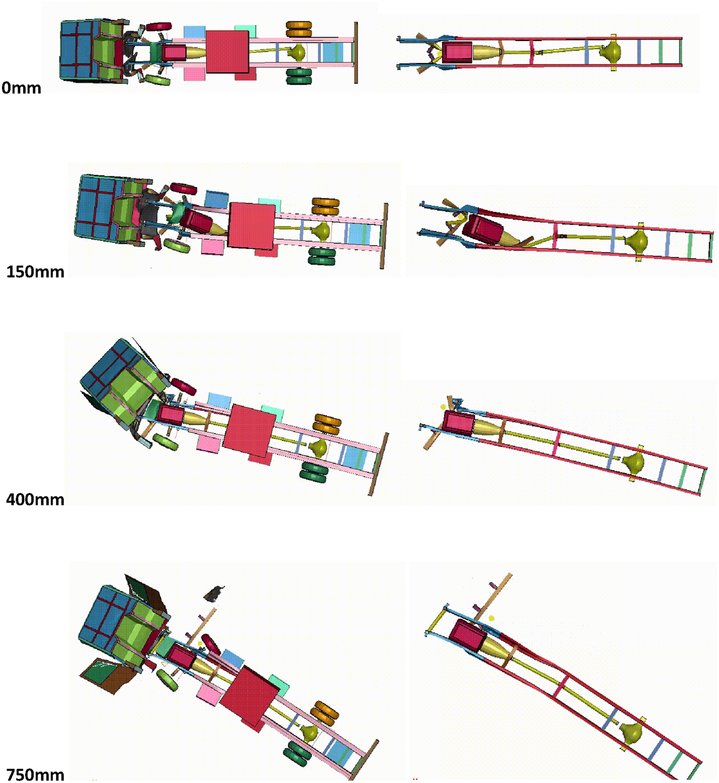

As for the N1 simulations, according to the momentum- and force-time plots (Figure 17) the direct shock of the engine to the bollard creates the highest force peaks for the configurations 0 mm (“centred”) and 150 mm (“non-centred”). Nevertheless, for the 400 mm “beam-centred” scenario, the force peak is much higher for the N2A simulations than for those of N1. This is because the frame beams are much stiffer in an N2A than in the N1 vehicles. The main reason is due to the presence of shock-absorbers in the N1 model, which reduce the frame beam crushing strength, that do not exist in the N2A model. Even if this could be model dependent, there is a more general trend according to which the frame shock absorbers are common for the N1 category vehicles Sebik et al. (2022) but not for the N2A category vehicles Sebik and Kodajkova (2023).

Figure 17.

The momentum-time plot (on the left) and the force-time plot (on the right) for the N2A simulations for the four different impact configurations: 0 mm (“centred”), 150 mm (“non-centred”), 400 mm (“beam-centred”) and 750 mm (“outlying”).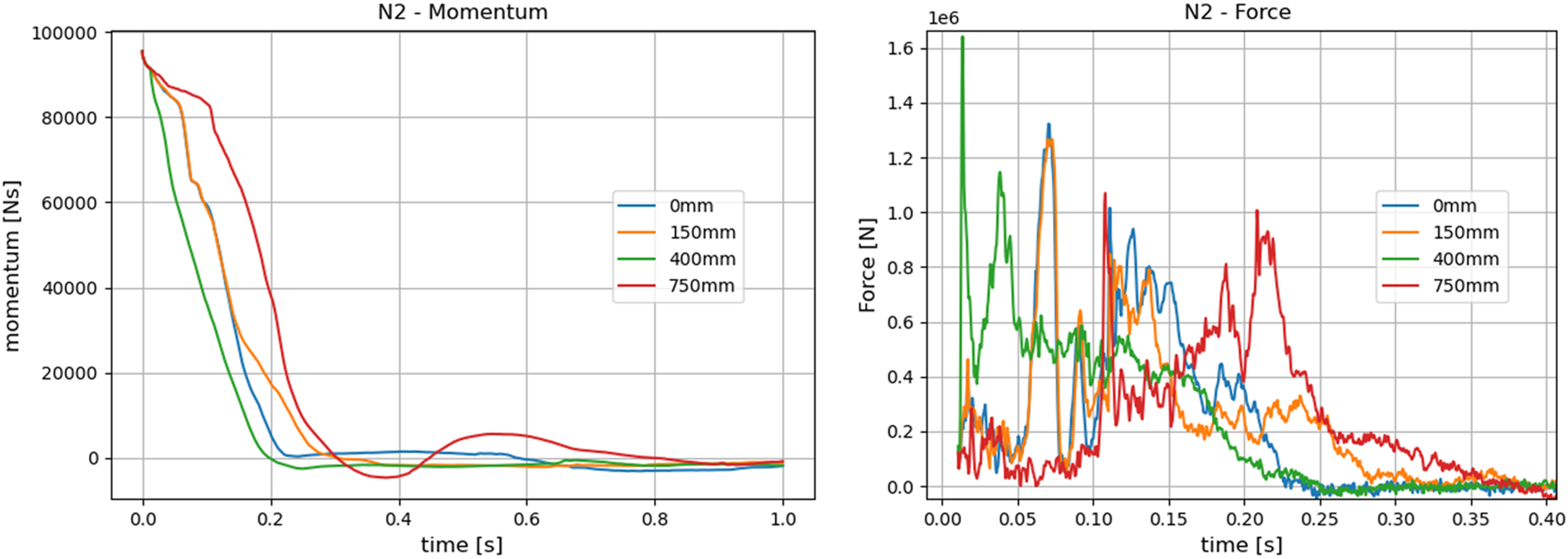

The 750 mm (“outlying”) scenario, not analysed in the N1 simulations, exhibits another very different behaviour, where unlike in the other scenarios, the force peak is due to the bollard interacting with the first wheel axle.

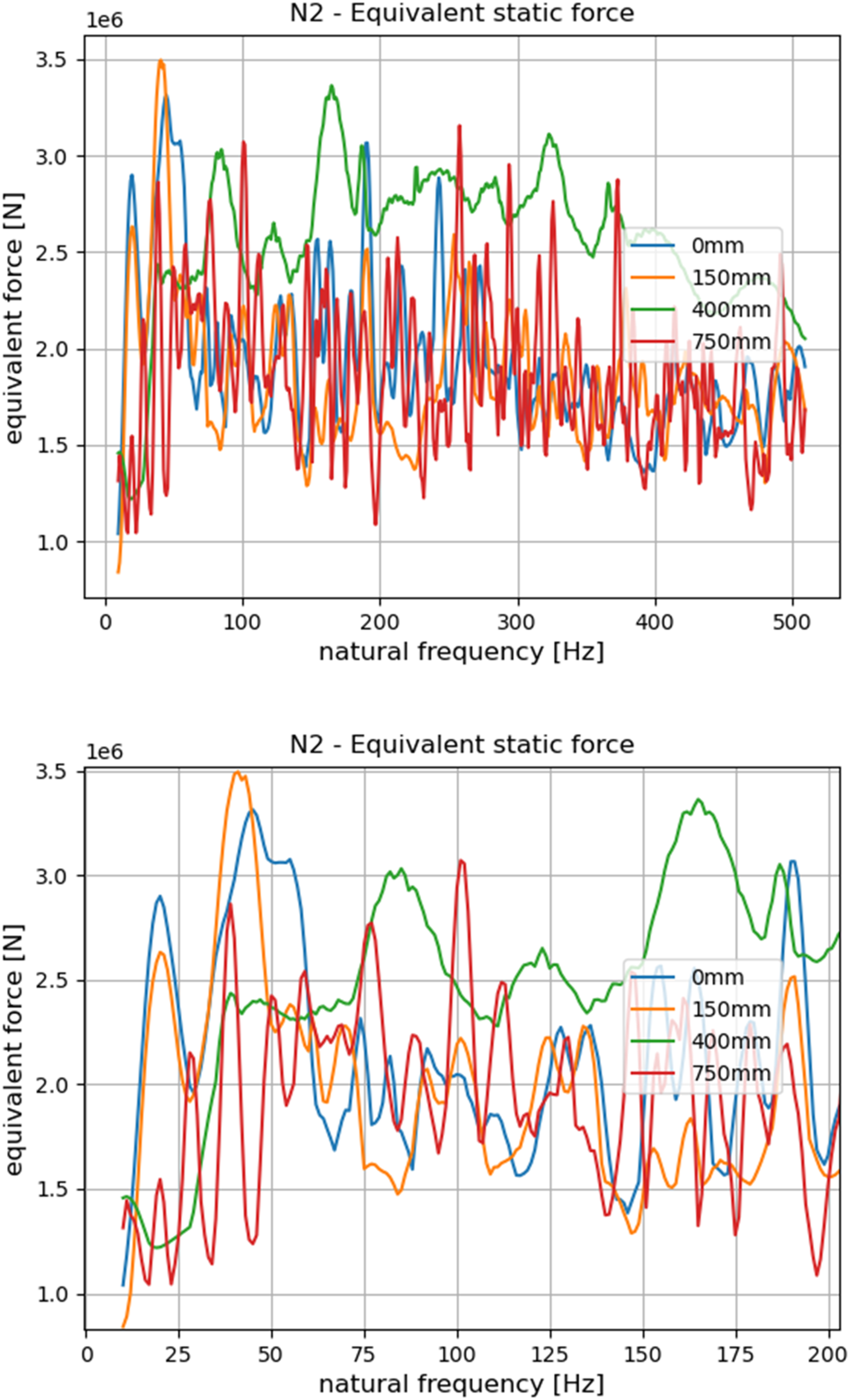
In the Figure 18 the “dynamic load factors” (DLF) depending on the barrier’s natural frequency (Section “Computation of the force-time loading function”) are presented for the four configuration considered above. The “equivalent static load” is presented in the Figure 19. It is important to stress that the “equivalent static load” graph is equal to the DLF graph scaled by the force peak value. Therefore, some scenarios can have lower values of the DLF (e.g. 400 mm “beam-centred”) but have high values of the “equivalent static load” due to a high force peak, or vice versa, high DLFs compensate the fact that the peak force is smaller.

Figure 18.

The dynamic amplification effect depending on the natural frequency of the barrier system for the N2A simulations for the four different impact configurations: 0 mm (“centred”), 150 mm (“non-centred”), 400 mm (“beam-centred”) and 750 mm (“outlying”).

Figure 19.

The “equivalent static force” depending on the natural frequency of the barrier system for the N2A simulations for the four different impact configurations: 0 mm (“centred”), 150 mm (“non-centred”), 400 mm (“beam-centred”) and 750 mm (“outlying”). The top figure presents the results for the frequencies up to 500 Hz and the bottom figure focuses to frequencies up to 200 Hz, in order to distinguish better the different curves for lower frequencies, which are expected to be more representative of the real barriers.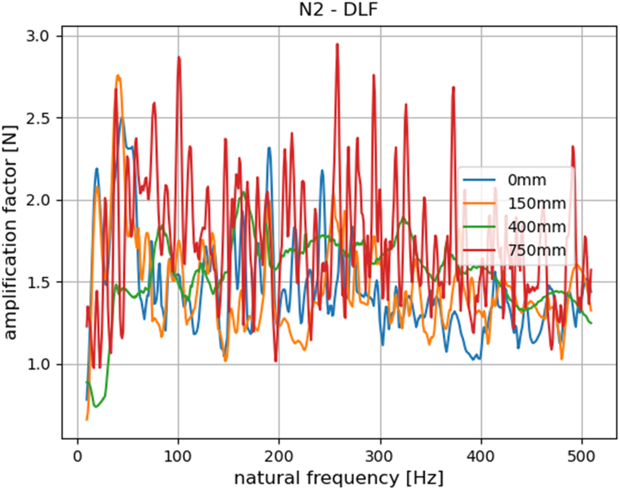

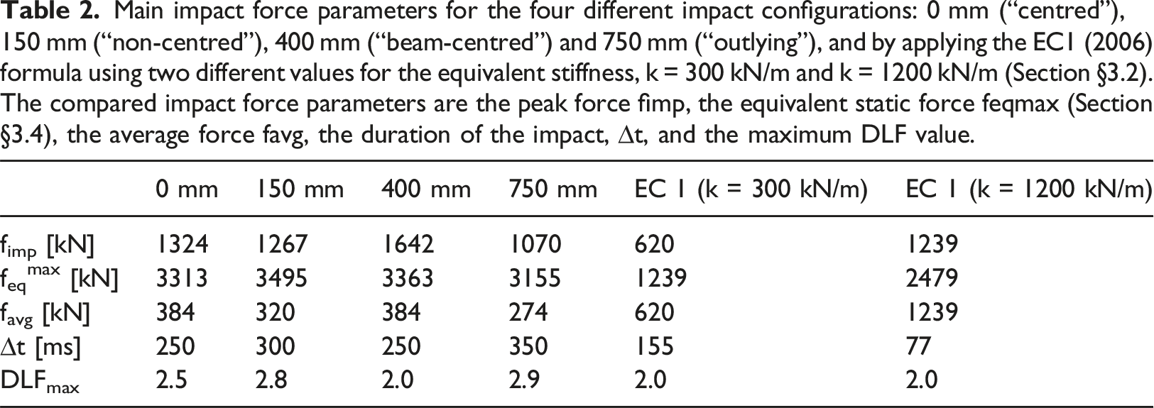
Table 2 compares the simulation results in terms of the peak impact force, f_imp, and the equivalent static force f_eq^max (Section “Barrier response”) with the impact force parameters, obtained with the EC1 (2006) formulas (Section “Analytical estimations for the impact force”). Like for the N1 simulations (Section “Results for the vehicle of N1 category”), the value of the impact duration, ∆t, and the average impact force, f_avg are also compared.

Table 2.

Main impact force parameters for the four different impact configurations: 0 mm (“centred”), 150 mm (“non-centred”), 400 mm (“beam-centred”) and 750 mm (“outlying”), and by applying the EC1 (2006) formula using two different values for the equivalent stiffness, k = 300 kN/m and k = 1200 kN/m (Section §3.2). The compared impact force parameters are the peak force fimp, the equivalent static force feqmax (Section §3.4), the average force favg, the duration of the impact, ∆t, and the maximum DLF value.

	0 mm	150 mm	400 mm	750 mm	EC 1 (k = 300 kN/m)	EC 1 (k = 1200 kN/m)
f_imp [kN]	1324	1267	1642	1070	620	1239
f_eq^max [kN]	3313	3495	3363	3155	1239	2479
f_avg [kN]	384	320	384	274	620	1239
∆t [ms]	250	300	250	350	155	77
DLF_max	2.5	2.8	2.0	2.9	2.0	2.0

Analysis

General trends

Both simulations sets, N1 (Section “Results for the vehicle of N1 category”) and N2A (Section “Results for the vehicle of N2A category”), conclude that the “centred” scenarios are globally the most penalizing. This is particularly true for the N1 case, both, in terms of the maximum force and by taking into account the dynamic amplification (through the DLF) in terms of the “equivalent static load”.

In the N2A simulations, the scenarios 0 mm (“centred”) and 150 mm (“non-centred”) exhibit similar behavior in all aspects. They are characterized by a strong direct interaction between the engine and the bollard, the source of the highest impact forces. Nevertheless, in terms of the force peaks, the highest is obtained with the 400 mm (“beam-centred”) scenario, in the beginning of the impact due to a high stiffness of the frame beam being hit directly. For this case, the “equivalent static load” is also higher than for the more “centred” scenarios, for the barrier’s natural frequencies over 60 Hz, whereas it is much lower for frequencies below 60 Hz. The “outlying” scenario is the least penalizing in terms of force peaks, but also in terms of “equivalent static forces” except for very low frequencies and for some peaks at some specific frequencies.

The results show that the “equivalent static load” is strongly dependent on the barrier’s natural frequencies. However, the natural frequencies of a barrier are not easy to be determined because they can be significantly influenced by the barrier’s foundation design and the surrounding soil conditions. If the bollard considered in this study (Figure 5) was perfectly anchored in the ground, its first natural frequency would be expected to be between 80 Hz and 120 Hz, depending also on the material used (usually a bollard is a steel shell filled with concrete). Due to the foundation flexibility, the first natural frequency of the bollard system could be much lower. On the other hand, the natural frequencies could be also higher for different bollard geometries (e.g. a bigger diameter).

Regarding the dynamic amplification effects, assessed through the DLF values, the general trend is that they are smaller than two only for low frequencies (i.e. < 50 Hz for the N1 case and < 20 Hz for the N2A case) and that they can approach or exceed the value of three for higher frequencies. As explained in the Section “Barrier response”, the DLF is bounded by the value of two only for simple single-peak force-time functions. Therefore, for realistic impact force-time functions, the DLF should be computed specifically for each scenario of interest.

Because of the dynamic amplification effects represented by DLF, potentially higher than the commonly assumed value of 2, an impact load should not be characterized by considering only the peak forces.

It is important to emphasize, that the used “equivalent static” approach considers a perfectly elastic barrier response and does not take into account any non-linear effect like cracking, plastic deformation or sliding.

N1 versus N2A

In terms of the peaks of the force-time functions, it is possible to observe that there is no significant difference between the N1 vehicles and the N2A vehicles. While in both cases force peaks of about 1 MN are commonly observed, the highest peak is actually obtained for the smaller N1 vehicle in the “centred” scenario (2.5 MN). Although the total impulse of the impact forces, which must equal the initial momentum of the vehicle, is approximately twice as big for the N2A vehicle as for the N1 vehicle, the N1 vehicle exhibits higher impact force peaks. This is because in the N1 simulations, the engine hits the bollard at a higher velocity than in the N2A simulations, where the initial deceleration of the vehicle is larger due to stiffer frame beams.

Namely, the N2A is a heavier duty vehicle, therefore its frame beams are stiffer and, in addition, do not have a shock absorbing part (i.e. crash boxes) like the N1 vehicle does. Therefore, in the N2A “beam-centred” simulation the frame stiffness is responsible for a force peak of 1.6 MN, whereas in the N1 equivalent case, the corresponding peak value is only 0.5 MN.

In Figure 20, the momentum-time plots for the “centred” scenarios N1 and N2A are compared. As expected, the total momentum decrease (equal to the total impulse of the impact force) for the N2A case is twice as big as the one for the N1 case, corresponding exactly to the mass ratio, with the impact velocity being the same (48 km/h). In Figure 20, it is observed that the momentum decrease at around 110 ms is almost the same, indicating that the average impact force before 110 ms is similar for the N1 and N2A cases.

Figure 20.

Momentum-time plot for the “centred” scenarios for the two different vehicles, N1 and N2A.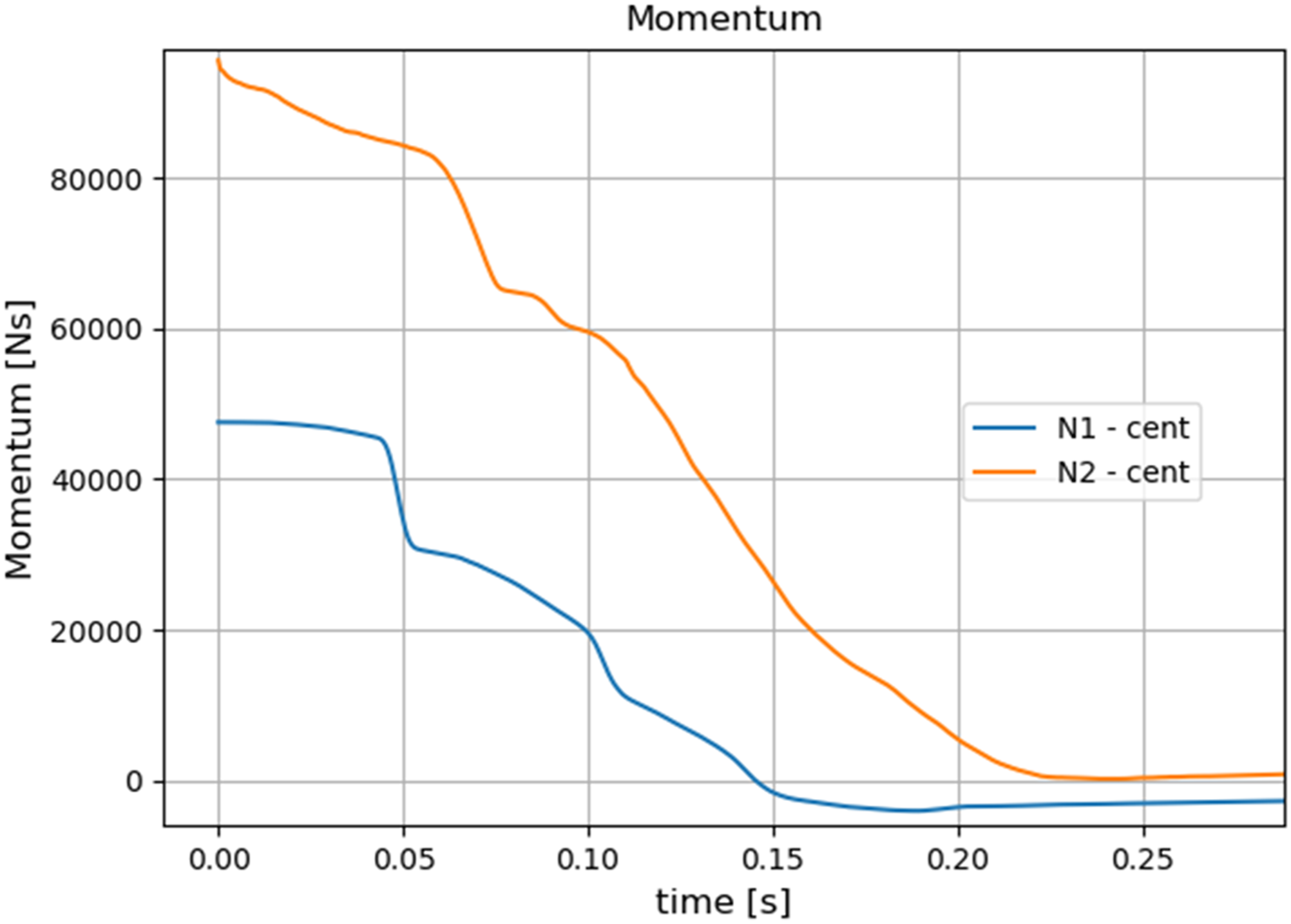

On the other hand, the corresponding force-time functions are very different (Figure 21). The N2A forces are bigger in the first 40 ms, but the N1 peak at 50 ms is almost twice as high as that for the N2A case. After the second engine-bollard shock (Section “Results for the vehicle of N1 category”) at around 110 ms, the N1 force drops significantly, whereas in the N2A case, it remains relatively high up to 200 ms

Figure 21.

Force-time plot for the “centred” scenarios for the two different vehicles, N1 and N2A.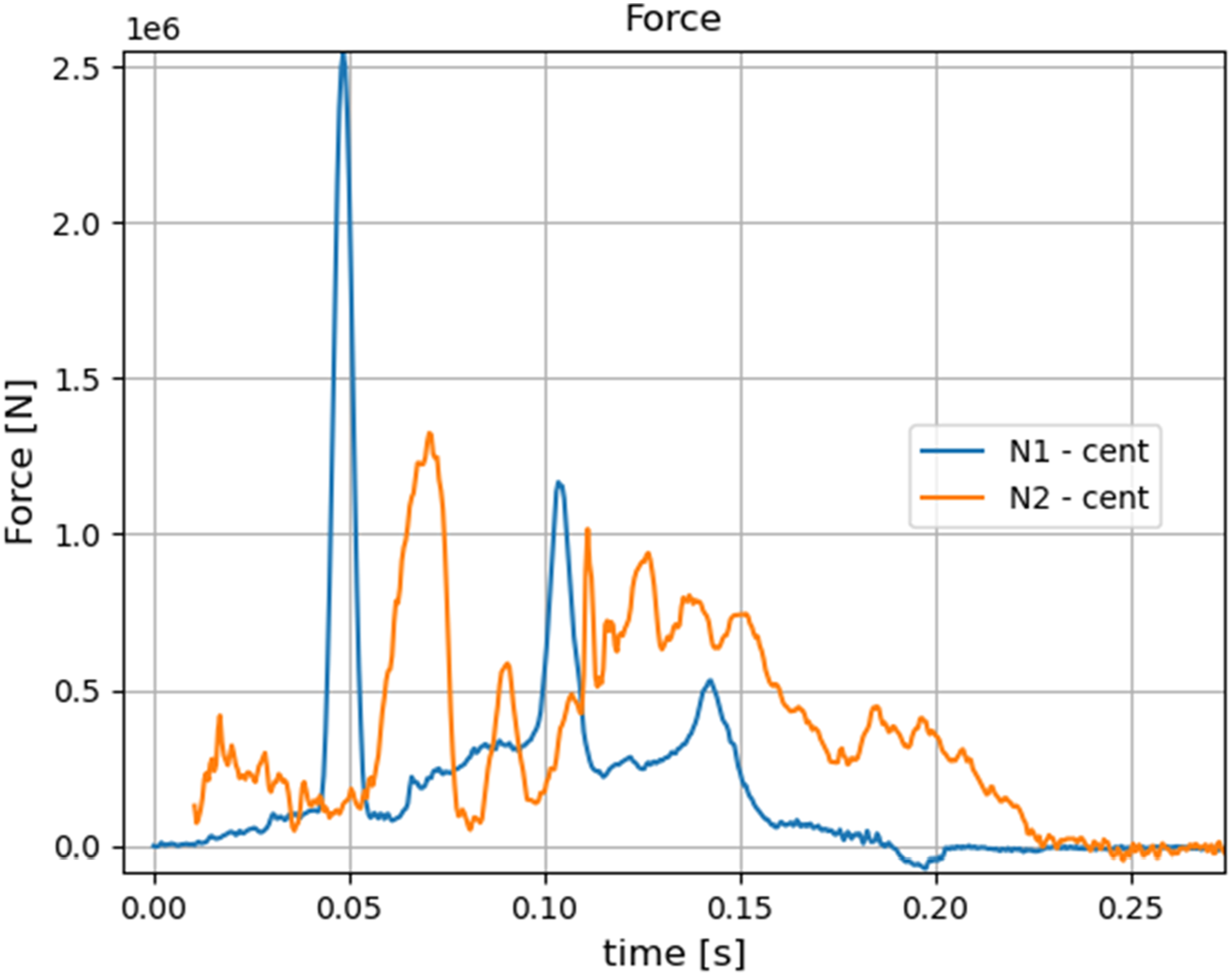

It is important to stress that the comparison of the force-time functions between different vehicles, N1 and N2A, is not entirely determinant for the load on the bollard. Namely, the N1 and N2A vehicles do not necessarily hit the bollard at the same height (i.e. vertical position with respect to the bollard), which means that the impact forces are not directly representative of the torque imposed to the barrier system. The ground clearance of N2A vehicles is expected to be about 25% higher than for the N1 vehicles, but this property is highly dependent on brand and model. In any case, the more penalizing height of the impact on a bollard for the N2A vehicles does not change the conclusion that a lighter N1 vehicle could eventually produce similar or higher stresses in the barrier system for some specific scenarios and barrier’s dynamic properties.

Analytical versus simulation approach

In the Tables 1 and 2, the main impact force characteristics between the analytical EC1 (2006) approach and the numerical simulations are compared. As the analytical approach is based on a significant simplification, considering the vehicle impact force being constant over the entire time interval, it gives significantly different results from the numerical simulations, which use a much more detailed representation of the vehicle crash load. In particular, a vehicle is composed of various components, each with different stiffness, making it difficult to represent a vehicle’s crashing behaviour with a single equivalent stiffness.

The main limitation of the EC1 (2006) approach is that it completely neglects force variations during the impact. In particular, there is no distinction between the average and the peak force, since the force is constant over a given time interval. Consequently, when comparing the analytical approach to the numerical simulations, it tends to overestimate the average force and to underestimate the peak force.

Nevertheless, by adjusting the vehicle equivalent stiffness (e.g., from 300 kN/m to 1200 kN/m), it is possible to obtain a more realistic peak force value, but at the cost of underestimating the impact duration. As the impact duration has a smaller influence on the barrier’s response for the situations of interest, it makes sense to prioritize higher vehicle equivalent stiffness values (e.g., 1200 kN/m) in order to match better the force peaks.

In summary, in this study the vehicle impact simulations provide in most scenarios higher peak forces than those of the EC1 (2006) approach. Additionally, for many frequency intervals, the DLFs obtained from the simulations actually exceed the value of two, an upper bound for simplified force-time functions considered by EC1 (2006).

Conclusions

Two recently developed generic vehicle models, one for the N1 category and the other for the N2A category, are used in this study to evaluate the vehicle crash response in terms of a force-time load on a rigid barrier. Contrary to the common perception that heavier vehicles are more detrimental to a barrier, our study reveals that this is not always the case. Namely, it is shown that the main impact force peaks are due to the engine hitting the barrier and that the severity of this shock depends especially on the velocity decrease in the beginning of the impact. The front parts of the N2A vehicle being stiffer than those of the N1 vehicle, the initial vehicle deceleration is higher and the N2A engine hits the barrier with a smaller velocity than in the N1 case.

Moreover, the study shows that the maximum impact force is not the only important indicator of an impact load on a barrier. Because realistic force-time functions can have several peaks, they can exhibit higher “dynamic load factors (DLF) than the value of two, the upper bound for simple single-peak (i.e., impulsive) force-time functions.

Because the impact load on a barrier is very dependent on the vehicle’s stiffness, the force-time load changes significantly for the different relative barrier-vehicle positions. Symmetrical (i.e., “centred”) impact scenarios, commonly used in physical experiments, often lead to the most severe load, but this outcome may depend on the barrier’s natural frequencies, themselves function of materials, dimensions, and the effect of foundations.

Our numerical simulations prove to be highly effective in replicating realistic vehicle impact behaviour and can be confidently used for virtual testing of security barriers. Given the complexity of crash phenomena, simulation tools are well suited for studying the sensitivity of the impact force load to various input parameters related to vehicle properties and impact scenarios.

In the future, the key findings of our study should be validated through more extensive sensitivity analyses, particularly by studying the influence of the impact velocity and the vehicle characteristics.

Footnotes

Declaration of conflicting interests

The author(s) declared no potential conflicts of interest with respect to the research, authorship, and/or publication of this article.

Funding

The author(s) received no financial support for the research, authorship, and/or publication of this article.

ORCID iDs

Damijan Markovic

Alessandro Scattina

Martin Larcher

References

Andrae

Markovic

Schumacher

, et al. (2024) Methodology for Numerical Simulations of Vehicle Impact on Security Barriers Considering Soil-Barrier Interaction. Luxembourg: EUR 31844, Joint Research Centre of the European Commission.

Ang

Lim

Kong

(2016) Test and numerical simulation of fixed bollard and removable bollard subjected to vehicle impact. 14th LS-DYNA Users Conference. Available at: https://lsdyna.ansys.com/wp-content/uploads/2022/12/test-and-numerical-simulation-of-fixed-bollard-and-removable-bollard-subjected-to-vehicle-impact.pdf.

Biggs

(1964) Introduction to Structural Dynamics. New York, NY: McGraw-Hill.

Chen

Xiao

, et al. (2015) Test and numerical simulation of truck collision with anti-ram bollards. International Journal of Impact Engineering 75(75): 30–39.

Chen

Fang

, et al. (2018) Numerical analysis of collision between a tractor-trailer and bridge pier. International Journal of Protective Structures 9(4): 484–503.

EC1 (2006) European Committee for Standardization (CEN) (2006) Eurocode 1. Actions on Structures, Part 1-7: General Actions-Accidental Actions. Brussels: European Committee for Standardization.

Gonzales

Kopacka

Kolman

, et al. (2021) Partitioned formulation of contact-impact problems with stabilized contact constraints and reciprocal mass matrices. Int J Numer Methods Eng. 2021 122: 4609–4636.

(2017) An assessment of current maximum impact force models for anti-ram bollard systems subjected to truck impact. International Journal of Protective Structures 8(3): 368–383.

Sun

(2014) Numerical investigation of K4-rating shallow footing fixed anti-ram bollard system subjected to vehicle impact. International Journal of Impact Engineering 63(63): 72–87.

10.

ISO 22343 (2023) Security and Resilience — Vehicle Security Barriers — Part 1: Performance Requirement, Vehicle Impact Test Method and Performance Rating. Geneva: Standard ISO 22343-1:2023.

11.

JRC web page (2024) Data and Tools to Counter Terrorism - Hostile Vehicle Mitigation - Generic Vehicle Models. Brussels: Joint Research Centre of the European Commission. https://counterterrorism.ec.europa.eu/hvm/generic-vehicle-models.php.

12.

Karlos

Larcher

Solomos

(2018) Guideline: Selecting Proper Security Barrier Solutions for Public Space Protection. Brussels: EUR 113778, Joint Research Centre of the European Commission.

13.

Kinney

Linzell

O’Hare

(2014) Assessment of load sharing members in an anti-ram bollard system. International Journal of Protective Structures 5: 417–433.

14.

Ravedati

(2023) MSc thesis report, Politecnico di Torino. https://webthesis.biblio.polito.it/29118.

15.

Saraceno

(2023) MSc thesis report, Politecnico di Torino. https://webthesis.biblio.polito.it/26326.

16.

Sebik

Kodajkova

(2023) Generic Vehicle Model N2A & N3D. Brussels: JRC135531, Joint Research Centre of the European Commission.

17.

Sebik

Popovic

Kleteckova

(2022) Generic vehicle model N1. In: JRC130165. Brussels: Joint Research Centre of the European Commission.

18.

Security by design (2022) Security by Design: Protection of Public Spaces from Terrorist Attacks. Brussels: Joint Research Centre of the European Commission.

19.

Spizzirri

(2023) MSc thesis report, Politecnico di Torino. https://webthesis.biblio.polito.it/29119.

20.

Valsamos