Sage Journals: Discover world-class research

Abstract

Explosive loading in a confined internal environment is highly complex and is driven by nonlinear physical processes associated with reflection and coalescence of multiple shock fronts. Prediction of this loading is not currently feasible using simple tools, and instead specialist computational software or practical testing is required, which are impractical for situations with a wide range of input variables. There is a need to develop a tool which balances the accuracy of experiments or physics-based numerical schemes with the simplicity and low computational cost of an engineering-level predictive approach. Artificial neural networks (ANNs) are formed of a collection of neurons that process information via a series of connections. When fully trained, ANNs are capable of replicating and generalising multi-parameter, high-complexity problems and are able to generate new predictions for unseen problems (within the bounds of the training variables). This article presents the development and rigorous testing of an ANN to predict blast loading in a confined internal environment. The ANN was trained using validated numerical modelling data, and key parameters relating to formulation of the training data and network structure were critically analysed in order to maximise the predictive capability of the network. The developed network was generally able to predict specific impulses to within 10% of the numerical data: 90% of specific impulses in the unseen testing data, and between 81% and 87% of specific impulses for data from four additional unseen test models, were predicted to this accuracy. The network was highly capable of generalising in areas adjacent to reflecting surfaces and as those close to ambient outflow boundaries. It is shown that ANNs are highly suited to modelling blast loading in a confined internal environment, with significant improvements in accuracy achievable if a robust, well distributed training dataset is used with a network structure that is tailored to the problem being solved.

Keywords

Artificial neural network confined blast load internal explosion machine learning specific impulse

Introduction

Background

Recent high-profile terrorist incidents, such as the Manchester Arena bombing (2017, 22 fatalities) and the Brussels Airport attacks (2016, 33 fatalities), involved the use of high explosives detonated in a crowded internal environment (Ben-Ezra et al., 2017; Kwon et al., 2017). Whilst the payload from vehicle-borne improvised explosive devices (VBIEDs) is considerably larger than those from person-borne explosives, the effects of a VBIED attack can be mitigated by enforcing a safe stand-off distance through the use of hardened security checkpoints and anti-vehicle barriers (Cormie et al., 2009). Whilst security checkpoints can also deter or prevent access to those intending to use person-borne explosives, they remain impractical for sites where large volumes of people require ready access, for example, airport pick up and drop off zones, train stations and concert halls.

Accurate prediction of the blast load arising from detonation of a high explosive remains a crucial step in assessing structural response (Rigby et al., 2019) and human injury (Pope, 2011). Detailed maps of the peak loading in an internal environment, and a comprehensive understanding of the factors affecting the magnitude of this loading, will allow for better provision of (active) mitigation systems, and will assist in planning interior layouts for enhanced (passive) blast protection strategies. Accordingly, a tool that can rapidly and accurately predict the complex loading in a crowded space is vital for risk-based engineering practice.

Existing semi-empirical approaches for predicting blast parameters, for example, the Kingery and Bulmash method (Kingery and Bulmash, 1984) and ConWep (Hyde, 1991), are known to be accurate only for far-field, geometrically simple scenarios (Rigby et al., 2014b).

When an explosion occurs in a complex environment, coalescence of multiple shock fronts that have reflected off or diffracted around obstacles is highly nonlinear (Larcher and Casadeia 2010) and hence simple superposition methods are unsuitable. Whilst methods for predicting confined loading exist in current design guidance, such approaches can only be used to calculate the average pressure acting on a single internal wall (assumed to be uniformly distributed and neglecting the walls parallel and opposite to the surface in question (US Department of Defence [US DOD], 2008), or the decay of quasi-static pressures, again averaged throughout the domain, for situations with high degrees of confinement and therefore low venting area (Anderson et al., 1983). Clearly, a more refined approach is required to consider situations which feature considerable interaction of blast waves, multiple reflections and development of increased specific impulses near the walls and the corners of the domain. Computational fluid dynamics (CFD) approaches offer the potential to develop a comprehensive and accurate description of an internal blast load, however it is impractical to use such approaches to inform risk-based engineering owing to the relatively high associated computational cost.

There is therefore the need to develop a predictive approach with the accuracy of a physics-based numerical scheme and the low computational cost of a semi-empirical method. Artificial neural networks (ANNs) are suitable as they have a proven ability to accurately predict complex nonlinear problems for various scenarios with simulations times comparable to basic solvers (see Figure 1). Applications of ANNs include estimating thermal performance of buildings (Flood et al. 2004), predicting blast-induced ground vibrations (Shahri and Asheghi, 2018) and quantification of blast loading on a building behind a blast wall (Remennikov and Rose, 2007) or along simple city streets (Remennikov and Mendis, 2006). Despite a clear applicability, the use of ANNs for internal explosions remains largely unexplored.

Figure 1.

Desired performance of ANNs.

The first aim of this paper is to critically evaluate the design of an ANN trained to simulate a given internal blast scenario. This is achieved through consideration of how the training dataset is generated and formatted before being used in the development of the ANNs. Additionally, a range of network structures are developed using various neuron counts to identify an optimum network configuration. The second aim of the study is to demonstrate the applicability of ANNs for predicting blast loading in an internal environment. Predictions generated by the ANNs are directly compared to numerical data from 72 different explosive scenarios during the training process. This allows for a comprehensive evaluation of the network performance including an assessment of how the network’s accuracy is dependent on each of the input values. The best performing network configuration is then evaluated using unseen input data from four additional tests to show that the ANN approach is capable of simulating specific impulse with percentage errors that are comparable to alternative methods.

Artificial neural networks

The progression of experimental techniques and bespoke modelling methods enable the use of ANNs for solving complex non-linear problems, especially those where the functional relationship between the input variables and output parameters is unknown (Alizadeh et al., 2017). They have applications involving data mapping, regression, classification and image processing (Dogan et al., 2017; Lee et al., 2012). However, for this study, focus will be placed on feed-forward, backpropagation regression networks. Training will take place using a supervised learning regime that generates improvements to the ANNs predictive accuracy through comparisons between the model output and known targets.

ANNs are formed of many neurons that process information being translated via connections. An example of a typical network is shown in Figure 2, with a forward pass being from left to right. Each connection holds a numerical weight that defines how large the value being passed via a given connection is. At each neuron, the translated values from the incoming connections are summed with a predefined bias that provides the neuron with a baseline magnitude. Before this summation result is passed onto the next neuron, it is standardised by an activation function that helps to prevent the input variable’s magnitudes from skewing the results disproportionally. Hidden layers/neurons allow for the interdependencies of the input variables to be captured which enables predictions to be made for complex problems.

Figure 2.

Example artificial neural network indicating the key components.

A summary of this calculation process for a given neuron is shown in Figure 3. It should also be noted that due to how the regression network will be required to predict continuous values, the activation function used on the output layer of neurons will be linear so that the predictions remain unbounded. This differs from the sigmoid or rectified linear unit (ReLU) functions that are commonly used at each of the hidden or input neurons.

Figure 3.

Example mathematical procedure for a single hidden neuron. Adapted from Remennikov and Rose (2007).

Initially, all weights and biases are given random values. The process of backpropagation is then used as part of the training process to reduce the output prediction errors using a gradient descent algorithm. By passing the output prediction errors from the forward pass back through the network, the weights and biases responsible for the inaccuracy are identified and optimised.

Once training is complete, testing of the network can take place using unseen input patterns. Rapid predictions can be formed by the network in this stage as the weights and biases are no longer being updated. The number of training patterns used, the complexity of the problem being modelled, and the network architecture will all influence the accuracy of a trained network because each of these factors control its ability to generalise from the training dataset (Remennikov and Rose, 2007).

Literature review

Field experiments provide the best chance at capturing the complex wave interaction processes associated with confined internal environments. However, they require specialist equipment and expertise that can often be very costly, and therefore simplifications are required. Experimental work by Anthistle et al. (2016), for example, utilised symmetry of the testing domain in order to model only a quarter of the environment. Here, it was found that good reproducibility was achieved between each test and therefore the use of symmetry constraints was considered acceptable.

Alternative approaches include modelling the entire domain at a scaled size. Fouchier et al. (2017) adopted this approach, using a range of wooden test structures at a 1:200 scale to analyse various street arrangements. It allowed for direct comparisons between each road/building layout to be conducted in a safer and more economical way. Hopkinson-Cranz scaling laws (Cranz, 1926; Hopkinson, 1915) were also shown to provide good agreement for the free-field and straight road arrangements meaning the results could be used for validation work in the future. It has been shown that numerical modelling of blast loading in an internal environment is highly complex, with the presence of multiple reflections requiring many equations and mathematical relationships to be solved in parallel (Larcher and Casadeia, 2010).

In situations where multiple field tests are not suitable, mathematical modelling presents a means of obtaining predictions for an unbounded range of scenarios, however experimental data is still required to rigorously validate these numerical approaches. A study by Xu et al. (2018) developed codes for 1D, 2D and 3D models based on finite difference schemes to analyse various test problems. The 3D code was then validated against experimental data for a confined chamber to prove that the model produced reliable overpressure-time histories. Generally, the accuracy of these methods is controlled by the coarseness of the element mesh forming the environment or the step size used in the calculation process. This is discussed further by Caçoilo et al. (2018), who studied the propagation of blast waves inside a survival blast chamber using an LS-DYNA numerical model. Through comparing the numerical results to a physical experiment, the authors reported specific impulse errors below 19% when using a mesh size of 3.25 mm. A finer mesh may improve on this further, however there is a trade-off between accuracy and computation time that will change based on the general arrangement of the simulations and intended use of the results. In this case, for the highly complex wave interaction processes that within the chamber, the paper shows how numerical methods are able to provide reasonable predictions for blast loading parameters without the need for experimental programmes beyond the validation stage.

The continuous development of numerical methods is driven by the increasing use of probabilistic approaches for modelling blast scenarios. These approaches allow for the uncertainties associated with explosions to be accounted for in risk analyses or cost-benefit assessments which ultimately makes them very useful for blast design and building appraisal (Netherton and Stewart, 2016). An example of this approach is detailed in a study by Alterman et al. (2019) where ProsAir was used to estimate blast loads, 1 m above the floor resulting from the detonation of an improvised explosive device (IED) in a typical ground floor foyer of a commercial or government building. A Monte-Carlo analysis framework was used to provide distributions of the model input parameters so that various conclusions could be made about the domain based on the likelihood of certain attacks taking place (Alterman et al., 2019). The need to simulate the same environment with a large number of varying input parameters does not lend itself to this sort of numerical approach as the computation times were reported to be between of 0.07 and 29.52 hrs for each model. A fast running deterministic model would therefore help to expedite the process of environment evaluation whilst also increasing the number of input parameters that could be considered.

Recent studies, for example, Gault et al. (2020), have been focussed on provide new methods for complex environment predictions using experimental records to form relationships between various blast parameters. The targeted benefit being that they can quickly produce reasonable outputs without a significant loss of accuracy. In this case, around 15% error is achieved for a tool that is flexible to allow the user to define a mesh and domain size in addition to a charge size and location.

Artificial neural networks (ANNs) present an alternative approach to providing rapid analyses without the need for relationships to be derived manually. The two broad categories for their use in blast engineering are for assessments of localised structural response to blast loads and for the prediction of key blast parameters. With the focus of this study being on the latter, papers by Remennikov and Rose (2007) and Remennikov and Mendis (2006) indicate that high predictive accuracy can be achieved both behind blast walls and along simple city streets. The former reports correlation coefficients in testing of 0.997 for overpressure, and 0.998 for specific impulse. Here the correlation coefficient is a numerical indication of the agreement between the output predictions and targets, with a value of 1 suggesting total agreement. This was achieved using two hidden layers in fully connected regression networks.

Similarly, Flood et al. (2009) details the results from two separate studies that both looked at predicting blast loading parameters behind walls. The first utilised a dataset of 1365 training patterns and 252 testing patterns that were gathered from numerical simulations, whereas the second used 195 for training and five for testing from scaled experiments. It was found that the testing phase correlation coefficient for peak overpressure decreased from 0.996 to 0.830 as the dataset size was reduced. It is also noted that the experimental dataset contained a larger variability in the spacing between each data point. The generalisation capability of the network was therefore restricted due to the lack of data that is well distributed throughout the value boundaries associated with each input variable (Flood et al., 2009).

A study by Bortolan Neto et al. (2020) noted a similar conclusion as a network was trained to predict the mechanical response of mild steel plates experiencing localised blasts. Through supplementing sparse experimental data with validated numerical modelling data, it was found that a robust training dataset could be formed which included a greater amount of training patterns. The inclusion of a core of experimental data also helped to provide confidence that the network was modelling blast scenarios that are physically accurate. This stage therefore acted as validation for the developed ANNs.

Overall, a review of literature shows that the ability of ANNs to generate rapid predictions with engineering-level accuracy could benefit probabilistic methods that require consideration of the variability of key blast parameters. However, the need for a robust dataset means that numerical or experimental methods (rather than simple analytical tools) will still be required in the development of ANNs. Clearly an increase in computational power will also expedite the data generation and training/validation processes, hence ANNs are expected to remain advantageous over pure CFD approaches.

Numerical modelling

Validation of APOLLO Blastsimulator

Introduction and mesh sensitivity

Numerical analyses were performed using APOLLO Blastsimulator (‘Apollo’ hereafter). Apollo is an explicit CFD software which specialises in the simulation of high-dynamic flow problems (Fraunhofer EMI, 2018). The conservation equations for transient flows of compressible, inviscid and non-heat conducting, inert or chemically reacting fluid mixtures are solved using a second-order finite-volume scheme with explicit time integration. Features such as dynamic mesh adaptation (DMA), 1D-to-3D mapping and 3D-to-3D staged mapping allow for efficient use of computational resources. DMA is controlled through the specification of a ‘zone length’, $L$ , which represents the element size at the coarsest resolution level, and a maximum resolution level, $N_{m a x}$ . The ‘ultimate cell length’ is the element size at the highest resolution level and is given as $h = L 2^{- N m a x}$ . Apollo has been extensively validated for near-field blast (Pannell et al., 2019, 2020; Whittaker et al., 2019), and so this section is focussed on validation of Apollo’s far-field blast predictions.

A mesh sensitivity study was completed in order to determine required element sizes to achieve convergence. A series of numerical simulations were completed for a 0.35 kg hemispheres of PE4 (modelled as a 0.7 kg sphere in Apollo), located at a stand-off distance, $S$ , of 6 m (scaled distance $Z = 8.51$ m/kg^{$1 / 3$}) from a rigid reflecting surface. PE4 is a plastic explosive comprising 87% RDX and 13% mineral oil binder (Tyas, 2019) and was used throughout the mesh sensitivity analysis and validation using Apollo’s in-built model for C4 since the two explosives are nominally identical (Bogosian et al., 2016). In all numerical simulations the explosives were centrally detonated using the Chapman-Jouguet model and the mass of the detonator was not included.

The domain size was $6 \times 6 \times 6$ m, and eighth-symmetry was used, with symmetry planes located in the directions orthogonal and opposite to the reflecting wall, originating at the centre of the charge. In all models an integer number of zones was specified for each of the domain side lengths. Outflow boundaries were defined at the roof of the domain and the remaining boundary. A numerical pressure gauge was placed at the base of the wall directly opposite the charge centre. Apollo’s 1D module was used with the limit defined at one zone length from the gauge (for a zone length of 300 mm, the 1D stage extended 5700 mm from the charge centre), and the auto-staging module was used throughout. In total 24 simulations were completed with the mesh information summarised in Table 1.

Table 1.

Ultimate cell length (element size at highest resolution level) and number of elements (between charge centre and normal gauge location) for initial mesh sensitivity study, Z = 8.5 m/kg^1/3.

(a) Ultimate cell length (mm)
	Zone length (mm)
Res. level	1000	600	400	300	200
0	1000	600	400	300	200
1	500	300	200	150	100
2	250	150	100	75	50
3	125	75	50	37.5	25
4	62.5	37.5	25	18.75
(b) Number of cells between charge and target
	Zone length (mm)
Res. level	1000	600	400	300	200
0	6	10	15	20	30
1	12	20	30	40	60
2	24	40	60	80	120
3	48	80	120	160	240
4	96	160	240	320

Results from the mesh sensitivity analysis are shown in Figure 4, each sub-figure shows: peak overpressure; peak specific impulse and total analysis time (termed ‘wall time’), all plotted against the ratio of stand-off distance, $S$ , to ultimate cell length. The solid black line shows the average experimental value from Rigby et al. (2015) and the dashed line shows a 10% variation from the experimental value. More information on the experiments is provided below in Experimental validation.

Figure 4.

Mesh convergence study for 0.35 kg PE4 at 6 m stand-off from a rigid reflecting wall. Solid line indicates average experimental value (Rigby et al., 2015) and dashed line indicates 10% variation from the experimental value.

The study suggests that an ultimate cell length of $h = S / 240$ and $h = S / 40$ are required for 10% convergence in overpressure and specific impulse respectively. As this research focusses on predicting specific impulse values, the less-stringent convergence requirement of $h = S / 40$ is implemented in later analyses. Whilst this requirement can be relaxed to $h = S / 16$ in the near-field, that is, $Z < 0.5$ m/ ${kg}^{1 / 3}$ (Pannell et al., 2020), a value of $h = S / 40$ is considered appropriate (albeit conservative) for the range of scaled distances in this study.

The benefits of the DMA module can be seen when wall time is considered: at $h = S / 60$ a noticeable reduction in wall time occurs when going from 200 mm to 400 mm zone length. Higher resolution levels allow Apollo to efficiently allocate computational resource, therefore a minimum level of 3 and a minimum ultimate cell length of $h = S / 40$ are recommended, provided an integer number of zones are specified for each of the domain side lengths.

Experimental validation

Rigby et al. (2015) present a series of experimental trials where pressure gauges, embedded flush with the surface of a large, reinforced concrete bunker wall, were used to record reflected pressure histories from 0.18 to 0.35 kg PE4 hemispheres located 2 to 10 m from the bunker wall. The experimental set-up is shown in Figure 5. For this validation exercise, only data from the normally reflected gauge, ‘G1’, was used.

Figure 5.

Pressure gauge location and general test arrangement of experimental data (Rigby et al., 2015).

The experimental dataset consists of 19 tests at nine unique scaled distances, therefore nine numerical analyses were performed. In each, the domain size was a regular cube with side-length equal to the stand-off distance in each case. As in the mesh sensitivity study, eighth-symmetry was used, with symmetry planes located in the directions orthogonal and opposite to the reflecting wall, originating at the centre of the charge. Outflow boundaries were defined at the roof of the domain and the remaining side. A numerical pressure gauge was placed at the base of the wall directly opposite the charge centre. Further information for each of the validation models is presented in Table 2, including resolution level, ultimate cell length and resulting stand-off/cell length ( $S / h$ ) ratio.

Table 2.

Input parameters and meshing strategy used for validation models.

Stand-off (m)	Charge mass (kg)	Zone length (mm)	Res. level	Ultimate cell length (mm)	S/cell length
2	0.25	200	4	12.50	160
4	0.18	200	4	12.50	320
	0.25	200	4	12.50	320
	0.35	200	4	12.50	320
6	0.25	300	4	18.75	320
	0.29	300	4	18.75	320
	0.35	300	4	18.75	320
8	0.25	400	4	25.00	320
10	0.25	400	4	25.00	400

Results from example numerical analyses are compared to experimental data in Figure 6. Here, results from the 4 m stand-off scenarios are presented: PE4 hemispheres of 0.18 (a), 0.25 (b) and 0.35 kg (c) corresponding to scaled distances of 7.08, 6.35 and 5.68 m/ ${kg}^{1 / 3}$ respectively. It can be seen that the magnitudes and general form of the numerical pressure and impulse histories closely match the experiments giving confidence that Apollo is correctly modelling the mechanisms of normal reflection in far-field blast scenarios. In all cases, the well-known secondary shock (Rigby and Gitterman, 2016) can be seen to arrive later in the numerical models, indicating that afterburning of the explosive detonation products is being slightly underestimated (Schwer and Rigby, 2017, 2018). However, the effect of on peak specific impulse is negligible since the secondary shock consistently arrives during the negative phase.

Figure 6.

Experimental validation of numerical overpressure and specific impulse histories at 4 m stand-off for: (a) 0.18 kg, (b) 0.25 kg and (c) 0.35 kg PE4 hemispheres.

Additionally, a comparison of numerical and experimental scaled peak specific impulse values (divided by the cube-root of the charge mass) is presented in Figure 7. The numerically generated peak specific impulses can be seen to closely match the experimental data consistently across the entire range of scaled distance and therefore Apollo can be considered to provide accurate specific impulse values in this region of scaled distances, provided the mesh requirements outlined in Introduction and mesh sensitivity are satisfied.

Figure 7.

Validation of Apollo scaled peak specific impulse against experiments (Rigby et al., 2015).

Generation of dataset

Problem domain

A domain was selected in order to be representative of a typical internal environment whilst offering the capability to train and test an ANN over a wide range of input parameters and output targets. As such, preliminary testing led to a domain of $10 \times 7 \times 5$ m being specified, with rigid surfaces placed on the upper and lower surfaces (ceiling and floor), and two of the four walls, see Figure 8. The two remaining boundaries were specified to be ambient so sufficient venting is provided to the domain and energy increase through afterburning (Edri et al., 2013) and quasi-static pressure development (Anderson et al., 1983) is negligible. The domain can therefore be considered as ‘fully vented’ according to the definition in UFC 3-340-02 (US DOD, 2008). This ensures that loading durations are not excessive whilst also making the domain indicative of an environment with frangible glazing that shatters immediately upon impact, offering no resistance to the blast. This combination of boundary conditions allows the ANNs to be tested using a broad range of data that includes regions where pressure is alleviated through venting and also where pressure will stagnate and increase in magnitude due to confinement effects in the corners.

Figure 8.

Simulation model boundaries and dimensions.

Whilst the ANN will be trained on a single domain and layout, the network will be tested on its ability to generalise by considering a range of charge masses and locations. Inclusion of additional parameters relating to the domain itself, for example, room size and wall/reflecting surface configuration, is outside the remit of this study. However, the network architecture is highly adaptable and new parameters can be incorporated into the network by specifying a number of additional input nodes, provided the network demonstrates an ability to generalise to the initial reduced problem set.

Data harvesting and simulation specifications

Williams (2015) reported that most hand-held improvised explosive devices are ~5 kg hence, in this study TNT explosive masses between 3 and 10 kg were used, as in Table 3, using Apollo’s in-built model for TNT. The range of charges were modelled in nine locations that form a grid around the centre of the domain, as shown in Figure 9, and were detonated from a height of 1 m above the floor. These charge locations correspond to a minimum normal scaled distance of 0.93 m/ ${kg}^{1 / 3}$ (10 kg at 2 m) and a maximum normal scaled distance of 5.20 m/ ${kg}^{1 / 3}$ (3 kg at 7.5 m).

Table 3.

Training variable constraints.

Variable	Variable options
TNT charge sizes ( $k g$ )	3, 4, 5, 6, 7, 8, 9, 10
Charge locations (x, y) [z = 1]	(2.5, 2), (5, 2), (7.5, 2), (2.5, 3.5), (5, 3.5), (7.5, 3.5), (2.5, 5), (5, 5), (7.5, 5)

Figure 9.

Charge locations within the chosen domain on plan. Black boundaries locate the rigid walls, clear boundaries represent ambient/outflow conditions [plan view].

To comply with the findings of Introduction and mesh sensitivity, the ultimate cell length for specific impulse convergence should be $< 0.05$ m when the shortest distance between charge and a rigid boundary is 2 m ( $S / 40 = 0.05$ ). A zone length of 0.24 m and resolution level of 3 (ultimate cell length of 0.03 m) was therefore specified for all 72 models to satisfy the impulse convergence requirement for the $S = 2$ m cases, ensuring that $h = S / 40$ was not exceeded in any scenario. It was found that this combination of parameters allowed for all tests to be performed within a week of continuous simulation.

The positions of the gauges included in the sampling mesh will be explored as part of the study as they will directly influence the performance of the trained ANNs. The height of the gauges was set to be 1 m above ground level, that is, in line with the centre of the charge. Sampling data at a fixed height above the ground is a common technique for reducing complexity of the data harvesting process for studies using numerical analyses or practical experiments (Alterman et al., 2019; Gajewski and Sielicki, 2020). Additionally, this decision does not significantly alter the architecture and predictive ability of the ANN but considerably reduces the time required for training and validation.

Once the data had been harvested and compiled, it was randomly reordered and sorted into two subsets: one for training and one for testing. For this study, the former will utilise 75% of the data, with the remaining 25% left for testing. This ratio is typical for neural network studies as training percentages can range from 70% to around 85% depending on the quantity of data (Dehghanbanadaki et al., 2019; Zaleski and Prozument, 2018).

Output check

Figure 10 shows the locations of three points within the chosen domain, with Figure 11 displaying the associated pressure-time and impulse-time histories for an 8 kg TNT charge located in the centre of the domain. Also shown are the ConWep (Hyde, 1991) semi-empirical predictions for positive phase incident overpressure and specific impulse for comparison. Note that the negative phase (Rigby et al., 2014a) has been omitted from the semi-empirical predictions as verifiable relations in the near-field are unavailable (Bogosian et al., 2002). The results differ significantly from the simple free-air case as expected. Gauge (a) shows the arrival of two clear pressure peaks, one from the primary shock wave, followed by a reflection from each of the rigid walls which arrive concurrently due to the position of the gauge. Gauge (b) shows a single, dominant pressure owing to its close proximity to the charge. Gauge (c) shows a simple free-air-type blast load with low-level, late-time pressure loading due to the partially-confined nature of the domain. In all cases, the pressure load initially appears similar to the ConWep incident pressure, with significant differences developing thereafter. This demonstration gives confidence that the physical processes are occurring and being modelled as expected, and that there is a clear, tractable dependency of the results on gauge location.

Figure 10.

Charge positioning and labelled gauge locations of the model output check [plan view].

Figure 11.

Apollo overpressure-time and specific impulse-time histories for three gauges shown in Figure 10 and ConWep (Hyde, 1991) incident wave overpressure-time and specific impulse-time histories at the corresponding stand-off distances.

Development of artificial neural network

Base network structure

The feed-forward, backpropagation, fully connected network developed by this study is shown in Figure 12. To limit the amount of structural trial and error, the number of hidden layers was fixed at two, with the number of neurons being varied during the development of the ANN. Two hidden layers were specified as Remennikov and Rose (2007) found this arrangement to perform better than when one, or three hidden layers are used. The location of the point of interest within the domain, and the size and positioning of the explosive charge form the input pattern and the peak specific impulse forms the solitary output.

Figure 12.

Base regression network structure.

Bewick et al. (2011) found that the use of non-scaled input parameters leads to improved correlations between targets and predictions. Additionally, the errors related to charge size may be obscured if scaled values are used. As a result, non-scaled inputs have been specified for all networks being developed in this paper. The used ANN code was written in Python using the Tensor Flow package for Machine Learning. Table 4 shows the network parameters that remained unchanged when training the ANNs.

Table 4.

Fixed network parameters.

Activation function	ReLU (Linear at output)
Error function	Mean squared error
Gradient descent algorithm	AdaGrad
Learning rate	Variable
Number of training steps	1000
Training batch size	100
Dropout rate	0.1

The number of training steps used in this study dictates how many times the weights and biases are updated given the error obtained from a randomly selected batch of 100 input patterns. In addition to using L2 regularisation terms, dropout is utilised to prevent overfitting. A dropout rate of 0.1 determines the number of neurons that are excluded and not updated in a given step of the training process. This helps to prevent ‘brittle co-adaptations that work for the training data but do not generalise to unseen data’ (Srivastava et al., 2014). Once training is complete, the testing dataset will be simulated in a single batch so that the network is assessed with unseen data that does not impact the weights and biases.

The AdaGrad (Adaptive Sub-gradient Descent) algorithm has been chosen as it adapts the learning rate and therefore the magnitude of variable updates during training so that common features within the dataset have smaller impacts whilst the rare features have larger impacts (Hadgu et al., 2015). It can therefore produce well-trained ANNs for datasets featuring localised effects and wide variations in output values. Further information concerning this algorithm can be found in a paper by Duchi et al. (2011).

Dataset development

Performance evaluation

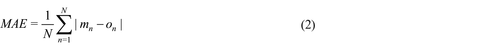
To explore multiple methods of forming the training dataset with limited computational expense, a preliminary development stage has been implemented. It involves the use of 27 of the 72 simulations corresponding to the 3, 6 and 10 kg tests for all 9 charge locations. Neural networks trained using the various datasets are given a fixed number of neurons per hidden layer (100) based on initial testing of the training process that found training times remain below 20 mins. Maintaining consistency with this parameter allows for effective performance comparisons to be made. Then, once the best performing dataset configuration is identified, the full range of charge sizes will be used to explore the impacts of changing the hidden neuron count before the network is evaluated at the conclusion of this paper. Performance evaluation will initially take place using two metrics. The first is the Youngs Correlation Coefficient, calculated using equation (1).

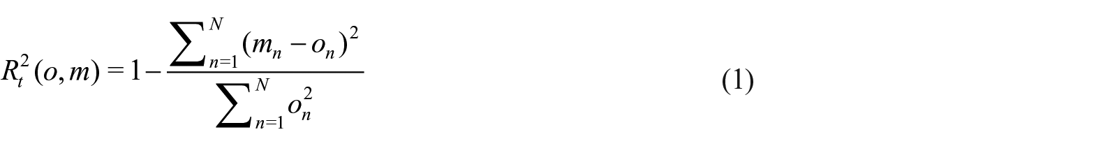
R_{t}^{2} (o, m) = 1 - \frac{\sum_{n = 1}^{N} {(m_{n} - o_{n})}^{2}}{\sum_{n = 1}^{N} o_{n}^{2}}

(1)

Where $R_{t}^{2}$ is the correlation coefficient, $m_{n}$ is the predicted specific impulse, $o_{n}$ is the target specific impulse that is obtained from the Apollo simulations and $N$ is the total number of data points. The second measure is the Mean Absolute Error, calculated using equation (2).

M A E = \frac{1}{N} \sum_{n = 1}^{N} | m_{n} - o_{n} |

(2)

Gauge spacing

The ability of a network to accurately model unseen situations is directly related to the quality and quantity of training data. The choice of a suitable resolution of gauge points is therefore key for the latter aspect, with each gauge providing a single data point that corresponds to the point of interest inputs of the network.

Figure 13 shows how gauges spaced at 1 m (a) provide 70 points per simulation, whereas a 0.5 m spacing (b) provides 280 points. For the 72 tests being simulated these correspond to either 5040 or 20,160 total input patterns for this domain. Sufficient gauge resolution is required to capture the spatial distribution of peak specific impulse across the entire domain, however, too fine a resolution will increase the prevalence of low magnitude impulse values and may limit the network’s ability to learn interdependencies between the two ‘point of interest’ input nodes and specific impulse. This would result in poorer predictions for higher-magnitude, spatially concentrated values of specific impulse, in particular in areas where shock fronts coalesce and superimpose, that is, along the two rigid walls of the domain and in the corner between them.

Figure 13.

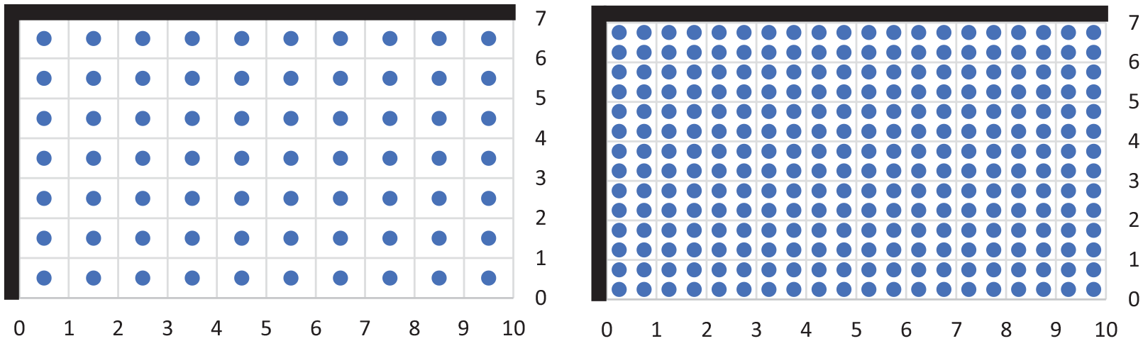
Gauge spacing options for the chosen domain [plan view].

Table 5 presents the achieved performance from networks trained using both dataset options. It is worth stating that despite the presented results being taken from the first network trained using the given conditions, the networks critiqued in this study have been trained multiple times to ensure that the reported performance statistics are not unique.

Table 5.

Network performance results achieved for ANNs using varied gauge spacing training datasets.

Network variable	Development stage	$R_{t}^{2}$	MAE (kPa.ms)
Gauge spacing: 1 m	Training	–	80.18
Gauge spacing: 1 m	Testing	0.9539	76.56
Gauge spacing: 0.5 m	Training	–	76.55
Gauge spacing: 0.5 m	Testing	0.9683	64.31

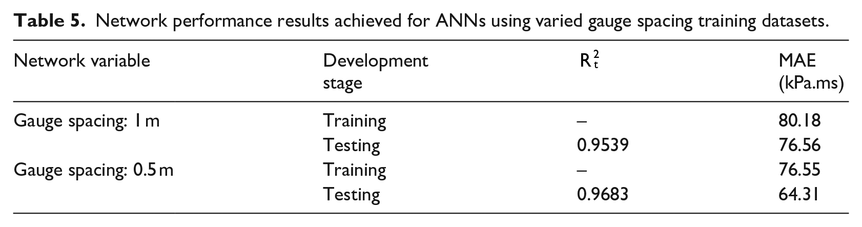
In this case, providing a greater number of data points with the finer mesh of gauges leads to an improved network performance in terms of MAE and correlation between targets and predictions. Overfitting is also avoided as in both instances, as the testing performance surpassed that which was achieved in training. All subsequent networks trained in this study therefore use data from gauges spaced 0.5 m apart with an origin at (0.25, 0.25).

Limited peak specific impulse

Figure 14 shows the distribution of testing predictions and targets for the network trained with 0.5 m gauge spacing with the solid black line representing a perfect prediction. This shows that larger specific impulse values appear to be predicted with considerably less accuracy. It is suggested that this is due to the reduced number of higher magnitude specific impulses included in the training dataset. The network weights and biases are updated less frequently for these predictions and, despite the AdaGrad descent algorithm being used to mitigate the implications of this, generalisation of the network for higher specific impulses appears unsatisfactory.

Figure 14.

Testing targets and predictions from the ANN developed using 0.5 m gauge spacing in the training dataset.

The largest magnitudes of specific impulse, directly around the charge, will far exceed any human injury criteria. It is also not practical to design a protective structure to resist such loading. The focus of the paper is therefore placed on the points outside of the zone immediately surrounding the charge. Through removing the influence of high specific impulses on the trained network variables, better predictive accuracy may be observed for points close to the dataset mean. To test this theory an impulse limit has been applied to the training dataset, defined as the mean plus two standard deviations ( $μ + 2 σ$ ). All targets above this value will be set to the limiting value itself, which for the charge sizes of 3, 6 and 10 kg, corresponds to 1088.5 kPa.ms.

The distribution of targets and predicted points for the network which utilises the impulse limit is shown Figure 15. It can be seen that the larger target values are still predicted with reduced accuracy compared to the rest of the data. However, when viewed against the results in Figure 14, it becomes clear that removing 44 data points that from the testing dataset that exceeded the impulse limit (of 1890 points in total) results in significant improvement. Table 6 presents the performance metrics from the initial and limited impulse analyses. In limiting the maximum impulse, the correlation coefficient has increased from 0.9683 to 0.9817, and the MAE has decreased from 64.31 kPa.ms to 56.99 kPa.ms. This proves that setting an impulse limit results in general improvements in the ability of the ANN to predict the entire dataset, and also leads to increased generalisation.

Figure 15.

Testing targets and predictions from the ANN developed using a specific impulse limit.

Table 6.

Testing network performance results with and without a specific impulse limit.

Network variable	$R_{t}^{2}$	MAE (kPa.ms)
No impulse limit	0.9683	64.31
Impulse limit = $μ + 2 σ$ = 1088.5 kPa.ms	0.9817	56.99

Network performance assessment

Accuracy evaluation

Following the configuration of the training dataset, an exploration of the neuron count for both hidden layers was performed. A training dataset made up of 15,120 points from all 72 tests using gauge spacing of 0.5 m was used with the associated impulse limit ( $μ + 2 σ$ ) also being applied. The aim here is to prove that ANNs are capable at modelling internal blast loading by training a network to a similar standard as other rapid analysis methods for blast loading predictions. It is shown by Rigby et al. (2014b) that the commonly used predictor ConWep (Hyde, 1991) can reproduce free-field values with a maximum error of 7%. Here, this shall be increased to a targeted 10% maximum error due to the added complexities of internal explosions and associated challenges to the numerical models. The formula for calculating the percentage error is given by Equation 3.

E_{n} (%) = \frac{| (m_{n} - o_{n}) |}{o_{n}} \times 100

(3)

Where $E_{n}$ is the percent error, $m_{n}$ is the predicted specific impulse, and $o_{n}$ is the target specific impulse that is obtained from the Apollo simulations corresponding to point $n$ .

Using this method of accuracy evaluation, the following sections will assess the performance of the ANNs with a view to quantifying typical differences between predicted and numerical data.

Hidden neuron count experimentation

Figure 16 shows that increasing the neuron count for both hidden layers leads to a continual decrease in the average percent error achieved when using the trained network with unseen inputs from the testing dataset. The number of points being predicted within a 10% error envelope also continuously increases as more neurons are added, albeit with decreasing improvements as the number of neurons increases.

Figure 16.

Error assessment of network predictions against unseen testing data: (a) mean percentage error, (b) percentage of points within a 10% error envelope.

Unlike many other studies using experimental data, here the training patterns comprise of incrementally stepped values in all variable space required for the network to operate. It is not common for a study to have such a detailed overview of the entire problem, and in many cases, it is commented by researchers that the reason for inconsistent performance is related to sparse datasets (Bewick et al., 2011). This may be why improvements in testing performance are seen in this manner for uncommonly large networks as the mean percentage error reaches 4.81% for a total of 3000 hidden neurons (MAE in testing was 29.9 kPa.ms for an average specific impulse of 591.5 kPa.ms).

Ultimately there is a diminishing return in performance improvement as the neuron count increases. The 1500/1500 structure required a training time of 190 mins to achieve the aforementioned accuracy level, whereas the 500/500 structure required 17 mins to achieve a mean percentage error of 5.90% and MAE of 36.3 kPa.ms. However, as the aim of this article is to demonstrate the effectiveness of ANNs for predicting blast loading in an internal environment, the most accurate network (1500/1500 neurons) is adopted for further study.

Figure 17 shows the training progress of the chosen network. It is clear that whilst rapid learning occurs to reduce the testing MAE from an initial value of $> 80$ kPa.ms to < 40 kPa.ms in ~180 steps, the additional steps, up to 1000, provide additional improvements that allow the network testing MAE to reach 29.9 kPa.ms. The network does not appear to be overfitted with the MAE at the end of the training process equalling 32.8 kPa.ms. This value is derived from the final batch of 100 randomly selected input patterns whereas the testing MAE is from all 5040 patterns that form the testing dataset. Whilst it is desirable to include a more detailed k-fold cross-validation and overfitting assessments, the aims of this paper are to demonstrate the use of ANNs for internal blast predictions and to evaluate the general design of the ANNs being used for internal modelling, and so these details are omitted in this manuscript.

Figure 17.

Training progress of the 5-1500-1500-1 structured network.

Impulse magnitude error variation

Figure 18 shows the 10% error envelope with the predictions and targets from testing for the 1500/1500 network. Details of how the error varies depending on specific impulse magnitude are given in Table 7. For specific impulses below 800 kPa.ms, over 90% of predictions are within 10% of the target value. For values $> 800$ kPa.ms this decreases to 84.5% of points within the 10% bracket. It is thought that the drop in performance could be linked to how there are only 760 data points with specific impulse above 800 kPa.ms in the testing dataset, which is relatively low compared to the other ranges. A similar distribution of magnitudes will present in the training dataset (since both are randomly generated) meaning the network variables are not being updated as many times for specific impulses $> 800$ kPa.ms as they are for other ranges. It is shown here that this leads to reduced prediction accuracy following training.

Figure 18.

Testing targets and predictions from the ANN developed with 1500 neurons in each hidden layer. The solid black line represents a perfect match between predictions and targets whilst the dashed lines represent a $\pm 10 %$ error envelope.

Table 7.

Variation of network predictive performance relative to the target specific impulse magnitude.

Peak specific impulse range (kPa.ms)	Number of testing dataset points	Percentage of training dataset points within percentage error range (%)
Peak specific impulse range (kPa.ms)	Number of testing dataset points	0 ≤ E < 5	5 ≤ E < 10	$10 \leq E < 20$	$E \geq 20$	E < 10
$i \leq \leq 400$	969	74.5	19.5	5.3	0.7	94.0
$400 < i \leq 600$	1718	76.5	13.5	6.2	3.8	90.0
$600 < i \leq 800$	1593	75.8	14.2	5.4	4.6	90.0
$800 < i$	760	51.2	33.3	10.8	4.7	84.5

For specific impulse values less than 400 kPa.ms, 94% of predictions are within 10% of the target value. This is the highest accuracy of any specific impulse range, despite being occupied by the second lowest number of testing data points (with the range $i >$ 800 occupying the lowest). This suggests that the network is more capable of predicting lower magnitude specific impulses than it is at predicting higher magnitude specific impulses, regardless of the amount of data points involved in training. It is hypothesised that the network is better able to predict lower impulse values ( $< 400$ kPa.ms) as these are regularly recorded at gauge locations nearest the ambient boundaries, therefore the network can rapidly learn relationships between gauge location and specific impulse, independent of charge size/location (i.e. it is dependent on only 2/5 of the input nodes and can rapidly generalise). In contrast, larger values of specific impulse are predominantly recorded around the position charge, which varies in each analysis, that is, the relationship is dependent on all five input nodes and therefore generalisation is more difficult with limited data.

Overall, the network predicted 89.9% of points in the testing dataset to within 10% of the target (numerical) impulse. This shows how the approach is largely successful even in this first assessment of its use for internal blast predictions.

Charge size error variation

The previous section leads into the need to assess if there is a variation in the predictive performance on the ANN based on the size of the explosive. Table 8 shows that for explosive masses less than 10 kg, performance is largely consistent, with only slight variations in accuracy for each range and charge mass. This shows that the network is able to generalise between the similar charge sizes well, particularly at the centre of the variable space (6 kg). However, for samples from the 10 kg tests, there is around a 5% reduction in the number of values being predicted with 10% error, despite there being a similar number of patterns used for each charge size in both training ( $\sim 1890$ ) and testing ( $\sim 630$ ) for all charges.

Table 8.

Variation of network predictive performance relative to the input charge size.

Charge size (kg)	Number of testing dataset points	Percentage of training dataset points within percentage error range (%)
Charge size (kg)	Number of testing dataset points	0 ≤ E < 5	$5 \leq E < 10$	$10 \leq E < 20$	$E \geq 20$	$E < 10$
3	644	66.9	23.3	8.7	1.1	90.2
4	605	75.6	15.3	5.3	3.8	90.9
5	614	77.0	13.8	5.1	4.1	90.8
6	621	77.6	14.0	4.2	4.2	91.6
7	646	74.7	15.9	6.2	3.2	90.6
8	649	69.1	20.2	6.5	4.2	89.3
9	596	70.8	19.6	6.4	3.2	90.4
10	665	65.7	19.9	9.2	5.2	85.6

This performance reduction may be caused by an increased number of higher peak specific impulse readings within the domain, which was shown in the previous section to lead to less accurate predictions. If this study were to have included charge sizes $> 10$ kg, it is anticipated that predictions for the 10 kg charge mass would improve since the dataset mean and standard deviation would also be increased. Therefore, the distributions of specific impulse from the 10 kg models would better compare to the mean. This highlights a slight deficiency in ANNs for this application in that they are less capable of predicting values towards the upper-end of the parameter range as discussed previously.

Charge location error variation

The 9 charge locations have also been analysed separately to identify any performance variations. These locations are shown in Figure 19, with the results from the analysis presented in Table 9.

Figure 19.

Labelled charge locations 1–9 within the chosen domain [plan view].

Table 9.

Variation of network predictive performance relative to the charge location.

Charge Location	Number of testing dataset points	Percentage of training dataset points within percentage error range (%)
Charge Location	Number of testing dataset points	$0 \leq E < 5$	$5 \leq E < 10$	$10 \leq E < 20$	$E \geq 20$	$E < 10$
1	538	69.7	18.0	7.8	4.5	87.7
2	523	69.6	21.4	6.5	2.5	91.0
3	593	69.0	21.4	4.4	5.2	90.4
4	583	73.6	15.4	7.1	3.9	89.0
5	557	66.8	18.9	10.2	4.1	85.7
6	588	64.5	21.7	9.9	3.9	86.2
7	566	80.4	12.0	4.4	3.2	92.4
8	526	81.6	13.5	3.0	1.9	95.1
9	566	74.4	17.8	4.6	3.2	92.2

The network appears to display some dependency on charge position, with the performance for positions 7 to 9 exceeding all others. The reason for this is not immediately clear, however it may be due to the larger distance between the charge locations and the longer outflow boundary (see Figure 19), thus increasing the prevalence of lower magnitude impulse values for which the network is better able to generalise. This theory does not extent to charge locations 1 and 4, however, which are the charge locations most remote from the shorter outflow boundary. It is suggested that this is due to the influence of the longer reflecting wall along the top edge of the domain, which will likely have a more significant effect on the pressure fields further downstream.

As the charge in location 5 is in the centre of the domain, this leads to a more balanced distribution of points, with some experiencing additional reflections and confinement effects, and others exhibiting more simple free-air-type loading. This will lead to a larger range of specific impulses to train over, hence making generalisation more difficult. Despite this, the model is still able to predict 85.7% of the specific impulses to within 10% of the numerical data (Table 9).

Final network design

Based on the findings outlined in the previous sections, the final network design is as follows:

Inputs: charge size (kg TNT); charge $x$ coordinate (m); charge $y$ coordinate (m); point of interest $x$ coordinate (m); point of interest $y$ coordinate (m)

Output: peak specific impulse at the point of interest (kPa.ms)

Hidden layer structure: 1500/1500 (two layers)

Activation function: ReLU (linear at output)

The associated network restrictions are then as follows:

Usable charge size range: 3 to 10 kg of equivalent TNT

Predictable points of interest: no closer than 0.25 m to a boundary and at 1 m height

Charge origin ( $z$ coordinate): 1 m

Predictable impulse limit derived from the training dataset (given as $μ + 2 σ$ ): ~1040.2 kPa.ms

Predicting blast loading in an internal environment using the ANN

With the network demonstrating a high level of accuracy when considering training data that was obtained from the original 72 simulations, it is essential that the approach is also tested on its ability to predict unseen data from new analyses. This involves using the trained network to predict four additional sets of values from scenarios where the variables are new to the network, but still within the respective variable spaces. The variable constraints that were implemented during training and testing are shown in Table 10, with Table 11 indicating how these values have been altered in each of the new test cases studied in this section.

Table 10.

Training variable constraints.

Variable	Range of permissible values
TNT Charge sizes (kg)	3, 4, 5, 6, 7, 8, 9, 10
Charge locations (x, y) [z = 1]	(2.5, 2), (5, 2), (7.5, 2), (2.5, 3.5), (5, 3.5)
Charge locations (x, y) [z = 1]	(7.5, 3.5), (2.5, 5), (5, 5), (7.5, 5)
Gauge spacing (m)	0.5
Gauge origin (x, y)[z = 1]	(0.25, 0.25)

Table 11.

Details of input variables used in additional unseen tests.

Variables	Test 1	Test 2	Test 3	Test 4
	New charge size	New gauge locations	New charge location	All new variables
Charge size (kg)	5.75	6	6	5.75
Charge location (x, y)	(5, 3.5)	(5, 3.5)	(4, 3)	(4, 3)
Gauge spacing (m)	0.5	1	0.5	1
Gauge origin (x, y)	(0.25, 0.25)	(0.5, 0.5)	(0.25, 0.25)	(0.5, 0.5)

Each of the first three tests are intended to investigate how the network copes with one change from the training variables. The final test then combines each of these alterations to present an entirely new input pattern to the network. Through assessing each of these variables it will highlight how well the network can interpret new inputs by relating them to the training variables it has seen before.

Figure 20 displays the obtained distributions from Apollo and the trained ANN. As per the previous simulations, the new models were run with a zone length of 0.24 m and resolution level of 3. Note that the maximum value of the colourbar is limited to 1000 kPa.ms for ease of interpretation, despite the limiting specific impulse used in the analysis equalling 1040.2 kPa.ms. The numerical and predicted specific impulse distributions are presented alongside a visualisation of percentage error. The error assessments of each test are provided in Table 12.

Figure 20.

(a) Numerical specific impulse distributions, (b) ANN predicted specific impulse distributions, and (c) percentage error. Colourbar maximum is set to 1000 kPa.ms for ease of interpretation (limiting specific impulse is 1040.2 kPa.ms).

Table 12.

Additional test percentage error results.

Test Number	Total data points	Percentage of additional test dataset points within percentage error range (%)
Test Number	Total data points	0≤E<5	$5 \leq E < 10$	$10 \leq E < 20$	$E \geq 20$	$E < 10$
1	280	63.2	23.2	9.3	4.3	86.4
2	70	65.7	21.4	10.0	2.9	87.1
3	280	52.9	33.6	9.6	3.9	86.5
4	70	52.8	28.6	12.9	5.7	81.4

It can be seen that the ANNs are able to reproduce the modelling results to a high level of accuracy across the entire domain both qualitatively and quantitatively. It is shown in Table 12 that at least 81.4% of the predicted impulses were within 10% of the numerical values for all four test models. Generally, the ANN is able to provide highly accurate predictions in areas where specific impulse is dominated by high magnitude, nonlinear superposition of reflected shocks, that is, along each reflecting wall and, in particular, in the corner between the two walls. In these regions, the complex interaction processes present many challenges to existing modelling approaches. Here, typical errors are $< 20 %$ for all locations along the reflecting walls, in all tests, indicating a good degree of generalisation of the predictive method. Furthermore, all tests show that an error of less than 10% is attainable near to the ambient boundaries and in areas of generally low specific impulse. It was shown previously that the ANN was more capable at generalising specific impulse predictions in regions of low complexity.

The agreement is less satisfactory in regions immediately adjacent to the charge, with errors consistently above 20%, albeit only in a relatively focussed area of the domain. The true magnitudes of these errors are not known due to the use of the impulse limit as explained previously. However, as discussed in Limited peak specific impulse, this is deemed acceptable as the areas surrounding the charge will be subjected to excessive specific impulses for which designing protective structures or preventing human injury would be impractical.

In total, each ANN was able to generate the predicted specific impulse distributions within 4 mins. The rapid generation of results and high level of agreement attained, both with the testing dataset and the additional test models presented in this section, shows that ANNs can be a highly useful tool for generating blast loading predictions in confined internal environments. The general structure of the network permits the inclusion of more complex analysis cases through the use of additional input nodes, for example, those representing the presence of internal reflecting obstacles, and more complex confinement and venting around the edges of the domain. Further exploration of alternative regularisation techniques, or activation functions that do not include a linearisation effect, also present many ways for future work to achieve more robust predictive performance for highly nonlinear cases.

Summary and conclusion

This study presents an evaluation of artificial neural networks (ANNs) for predicting the complex blast loading in a confined internal environment. Design of the ANN was rigorously evaluated through considerations of parameters such as gauge spacing (for the training and testing dataset), limited peak specific impulse, and number of hidden neurons, set domain size considered to be ‘fully vented’ according to the terminology in UFC 3-340-02 (US DOD, 2008).

Apollo Blastsimulator was used to gather training and testing data for the ANN. Firstly, Apollo was validated against available experimental data (Rigby et al., 2015) and shown to be in good agreement for far-field blast predictions. A full dataset was then harvested from 72 separate models from eight different charge sizes, each located at nine different positions within a $10 \times 7 \times 5$ m computational domain with floor, ceiling and two adjacent walls specified as rigid reflecting boundaries. Thus, 20,160 individual datapoints were generated, with 75% randomly assigned to train the network and the remaining 25% retained for testing.

It was found that both increasing the quantity of the available data and setting a limit on the maximum peak specific impulse (equal to the mean specific impulse plus two standard deviations) resulted in an improved performance of the network. Following this, the an optimised network structure was identified to include two hidden layers of 1500 neurons each, with five input neurons and a single output neuron. The network was able to predict the specific impulse for $\sim 90 %$ of the gauge locations to within 10% of the numerical values during the testing phase of the training process. It was found that the network was able to generalise for a wide range of specific impulse values, and was particularly accurate for areas of low specific impulse (e.g. those located close to the outflow edges of the domain), although its ability to generalise for larger specific impulses (and for the model with the largest charge mass) was inhibited by a general lack of high impulse datapoints for training.

The benefits of using ANNs to predict unseen data were clearly demonstrated with four new models. Here, the numerical analyses each took approximately 2 hrs, whereas the network was able to generate predictions within 4 mins. In each case, specific impulse was predicted to within 10% accuracy for between 81% to 87% of the gauge locations, with a high level of accuracy demonstrated along the rigid reflecting walls and in the corner between the two. Errors were found to be $< 20 %$ in all tests for every point that was not immediately adjacent to the charge. It has therefore been proven that ANNs are highly suited for predicting blast loading in a confined internal environment, with significant improvements in accuracy achievable if the network structure and training dataset are tailored to the problem being solved.

The ANN method is highly flexible and can be readily adapted to incorporate a wider range of input parameters. Extension of this method to account for charge shape effects, to predict loading at a range of heights within the domain, and to model different domain sizes with differing degrees of confinement, can be achieved by adding relevant input nodes to describe the new parameters. Such changes will not require substantial adjustments to the remaining architecture of the ANN, nor will the process of generating and format training/validation data differ from the methods we present in this article, and therefore the findings presented herein can also be considered as valid for ANNs developed to predict blast load parameters in scenarios which differ to those presented herein.

Footnotes

Acknowledgements

The authors wish to thank Dr Andrew Liew at The University of Sheffield for providing the artificial neural network code that has been adapted for use in this study.

Declaration of conflicting interests

The author(s) declared no potential conflicts of interest with respect to the research, authorship and/or publication of this article.

Funding

The author(s) received no financial support for the research, authorship and/or publication of this article.

ORCID iD

Samuel E Rigby

References

Alizadeh

Shahheydari

Kavianpour

, et al. (2017) Prediction of longitudinal dispersion coefficient in natural rivers using a cluster-based Bayesian network. Environmental Earth Sciences 76(2): 86.

Alterman

Stewart

Netherton

(2019) Probabilistic assessment of airblast variability and fatality risk estimation for explosive blasts in conﬁned building spaces. International Journal of Protective Structures 10(3): 306–329.

Anderson

Jr Baker

Wauters

, et al. (1983) Quasi-static pressure, duration, and impulse for explosions (e.g. HE) in structures. International Journal of Mechanical Sciences 25(6): 455–464.

Anthistle

Fletcher

Tyas

(2016) Characterisation of blast loading in complex, conﬁned geometries using quarter symmetry experimental methods. Shock Waves 26(6): 749–757.

Ben-Ezra

Hamama-Raz

Mahat-Shamir

(2017) Psychological reactions to the 2017 Manchester Arena bombing: A population based study. Journal of Psychiatric Research 95: 235–237.

Bewick

Flood

Chen

(2011) A neural-network model-based engineering tool for blast wall protection of structures. International Journal of Protective Structures 2(2): 159–176.

Bogosian

Ferritto

Shi

(2002) Measuring uncertainty and conservatism in simpliﬁed blast models. In: 30th explosives safety seminar, Atlanta, GA, USA, 13–15 August, pp.1–26.

Bogosian

Yokota

Rigby

(2016) TNT equivalence of C-4 and PE4: A review of traditional sources and recent data. In: 24th international symposium on military aspects of blast and shock (MABS24), Halifax, Nova Scotia, Canada, 19–23 September.

Bortolan

Neto

Saleh

Pickerd

, et al. (2020) Rapid mechanical evaluation of quadrangular steel plates subjected to localised blast loadings. International Journal of Impact Engineering 137103461.

10.

Caçoilo

Teixeira-Dias

Mourão

, et al. (2018) Blast wave propagation in survival shelters: Experimental analysis and numerical modeling. Shock Waves 28(6): 1169–1183.

11.

Cormie

Mays

Smith

(2009) Blast Effects on Buildings, 2nd edn, London: ICE Publishing.

12.

Cranz

(1926) Lehrbuch der Basllistik. Berlin, Germany: Springer.

13.

Dehghanbanadaki

Sotoudeh

Golpazir

, et al. (2019) Prediction of geotechnical properties of treated ﬁbrous peat by artiﬁcial neural networks. Bulletin of Engineering Geology and the Environment 78(3): 1345–1358.

14.

Dogan

Arslan

Ceylan

(2017) Concrete compressive strength detection using image processing based. Measurement 109: 137–148.

15.

Duchi

Hazan

Singer

(2011) Adaptive subgradient methods for online learning and stochastic optimization. Journal of Machine Learning Research 12(7): 2121–2159.

16.

Edri

Feldgun

Karinski

, et al. (2013) Afterburning aspects in an internal TNT explosion. International Journal of Protective Structures 4(1): 97–116.

17.

Flood

Bewick

Dinan

, et al. (2009) Modeling blast wave propagation using artiﬁcial neural network methods. Advanced Engineering Informatics 23(4): 418–423.

18.

Flood

Issa

RRA

Abi-Shdid

(2004) Simulating the thermal behavior of buildings using artiﬁcial neural networks-based coarse-grain modeling. Journal of Computing in Civil Engineering 18(3): 207–214.

19.

Fouchier

Laboureur

Youinou

, et al. (2017) Experimental investigation of blast wave propagation in an urban environment. Journal of Loss Prevention in the Process Industries 49: 248–265.

20.

Fraunhofer

EMI

(2018) APOLLO Blastsimulator Manual, Version: 2018.2. Freiburg, Germany: Fraunhofer Institute for High-Speed Dynamics, Ernst-Mach-Institut.

21.

Gajewski

Sielicki

(2020) Experimental study of blast loading behind a building corner. Shock Waves 30(4): 385–394.

22.

Gault

Sochet

Hakenholz

, et al. (2020) Inﬂuence of the explosion center on shock wave propagation in a conﬁned room. Shock Waves 30(5): 473–481.

23.

Hadgu

Nigam

Diaz-Aviles

(2015) Large-scale learning with AdaGrad on Spark. In: 2015 IEEE international conference on big data, Santa Clara, CA, USA, 29 October–1 November, Vol. 2, pp.2828–2830. IEEE.

24.

Hopkinson

(1915) British Ordnance Board Minutes, 13565. Kew, UK: The National Archives.

25.

Hyde

(1991) Conventional Weapons Effect Program (ConWep). Vicksburg, MS, USA: U.S Army Waterways Experimental Station.

26.

Kingery

Bulmash

(1984) Airblast parameters from TNT spherical air burst and hemispherical surface burst. Technical report, ARBRL-TR-02555, US Army Ballistic Research Laboratory, Aberdeen Proving Ground, MD, USA.

27.

Kwon

Chadha

Pellizzaro

(2017) Proximity and terrorism news in social media: A construal-level theoretical approach to networked framing of terrorism in Twitter. Mass Communication and Society 20(6): 869–894.

28.

Larcher

Casadeia

(2010) Explosions in complex geometries – a comparison of several approaches. International Journal of Protective Structures 1(2): 169–195.

29.

Lee

Park

Choi

(2012) Spatial prediction of ground subsidence susceptibility using an artiﬁcial neural network. Environmental Management 49(2): 347–358.

30.

Netherton

Stewart

(2016) Risk-based blast-load modelling: Techniques, models and beneﬁts. International Journal of Protective Structures 7(3): 430–451.

31.

Pannell

Panoutsos

Cooke

, et al. (2020) Predicting speciﬁc impulse distributions for spherical explosives in the extreme near-ﬁeld using a Gaussian function. Submitted for Possible Publication in International Journal of Protective Structures.

32.

Pannell

Rigby

Panoutsos

, et al. (2019) Predicting near-ﬁeld speciﬁc impulse distributions using machine learning. In: Proceedings of the 18th international symposium on interaction of the effects of munitions with structures (ISIEMS18), Panama City Beach, FL, USA, 21–25 October.

33.

Pope

(2011) The development of a quick-running prediction tool for the assessment of human injury owing to terrorist attack within crowded metropolitan environments. Philosophical transactions of the Royal Society B: Biological Sciences 366(1562): 127–143.

34.

Remennikov

Mendis

(2006) Prediction of airblast loads in complex environments using artiﬁcial neural networks. WIT Transactions on the Built Environment 87: 269–278.

35.

Remennikov

Rose

(2007) Predicting the effectiveness of blast wall barriers using neural networks. International Journal of Impact Engineering 34(12): 1907–1923.

36.

Rigby

Fay

Tyas

, et al. (2015) Angle of incidence effects on far-ﬁeld positive and negative phase blast parameters. International Journal of Protective Structures 6(1): 23–42.

37.

Rigby

Gitterman

(2016) Secondary shock delay measurements from explosive trials. In: Proceedings of the 24th international symposium on military aspects of blast and shock (MABS24), Halifax, Nova Scotia, Canada, 19–23 September.

38.

Rigby

Tyas

Bennett

, et al. (2014a) The negative phase of the blast load. International Journal of Protective Structures 5(1): 1–19.

39.

Rigby

Tyas

Curry

, et al. (2019) Experimental measurement of speciﬁc impulse distribution and transient deformation of plates subjected to near-ﬁeld explosive blasts. Experimental Mechanics 59(2): 163–178.

40.

Rigby

Tyas

Fay

, et al. (2014b) Validation of semi-empirical blast pressure predictions for far ﬁeld explosions – is there inherent variability in blast wave parameters? In: Proceedings of the 6th international conference on protection of structures against hazards, Tianjin, China, 16–17 October.

41.

Schwer

Rigby

(2017) Reﬂected secondary shocks: Some observations using afterburning. In: Proceedings of the 11th European LS-DYNA conference, Salzburg, Austria, 9–11 May.

42.

Schwer

Rigby

(2018) Secondary and height of burst shock reﬂections: Application of after-burning. In: Proceedings of the 25th Military Aspects of Blast and Shock (MABS25), The Hauge, Netherlands, 23–28 September.

43.

Shahri

Asheghi

(2018) Optimized developed artiﬁcial neural network-based models to predict the blast-induced ground vibration. Innovative Infrastructure Solutions 3(1): 34.

44.

Srivastava

Hinton

Krizhevsky

, et al. (2014) Dropout: A simple way to prevent neural networks from overﬁtting. Journal of Machine Learning Research 15(1): 1929–1958.

45.

Tyas

(2019) Blast loading from high explosive detonation: what we know and what we don’t know. In: Proceedings of the 13th international conference on shock and impact loads on structures, Guangzhou, China, 13–15 December.

46.

US Department of Defence (2008) Structures to resist the effects of accidental explosions. Working Paper UFC 3-340-02. Washington DC: US DoD.

47.

Whittaker

Klomfass

Softley

, et al. (2019) Comparison of numerical analysis with output from precision diagnostics during near-ﬁeld blast evaluation. In: Proceedings of the 18th international symposium on interaction of the effects of munitions with structures (ISIEMS18), Panama City Beach, FL.

48.

Williams

(2015) Enhancing the applicability of blast modelling and advice. International Journal of Protective Structures 6(4): 701–709.

49.

Kong

Zheng

, et al. (2018) Numerical method for predicting the blast wave in partially conﬁned chamber. Mathematical Problems in Engineering 2018: 1–17.

50.

Zaleski

Prozument

(2018) Automated assignment of rotational spectra using artiﬁcial neural networks. Journal of Chemical Physics 149(10): 104106.

Prediction of blast loading in an internal environment using artificial neural networks

Abstract

Keywords

Introduction

Background

Artificial neural networks

Literature review

Numerical modelling

Validation of APOLLO Blastsimulator

Introduction and mesh sensitivity

Experimental validation

Generation of dataset

Problem domain

Data harvesting and simulation specifications

Output check

Development of artificial neural network

Base network structure

Dataset development

Performance evaluation

Gauge spacing

Limited peak specific impulse

Network performance assessment

Accuracy evaluation

Hidden neuron count experimentation

Impulse magnitude error variation

Charge size error variation

Charge location error variation

Final network design

Predicting blast loading in an internal environment using the ANN

Summary and conclusion

Footnotes

Acknowledgements

Declaration of conflicting interests

Funding

ORCID iD

References