Sage Journals: Discover world-class research

Abstract

When researchers consider the relation between continuous predictors (e.g., perceived threat) and binary outcomes (e.g., being stopped by police), they typically adopt a means-focused approach, (a) attributing observed differences in binary outcomes to expected mean differences in continuous predictors and/or (b) predicting expected differences in binary outcomes using observed mean differences in continuous predictors. Because non-mean distribution moments of the continuous predictor (variance/skewness/kurtosis) also predict binary outcomes, this means-based approach can lead researchers to make inaccurate inferences about the relation between continuous predictors and binary outcomes and overlook viable cognitive explanations for individual or group differences in binary outcomes. We describe the extent to which differences in non-mean distribution moments for continuous predictors translate to differences in binary outcomes (Part I). We show that modeling non-mean distribution moments can change predicted binary outcomes (Part II) and inform existing psychological theory (Part III).

Keywords

scientific inference population distributions threshold models stimulus sampling manipulation checks

When researchers consider continuous predictors of binary outcomes—for example, perceived threat as a predictor of police stops—they typically adopt a means-focused approach. To the extent that researchers observe differences in a binary outcome, they might expect corresponding mean differences in the continuous predictor. Conversely, to the extent that researchers observe mean differences in continuous predictors, they might expect corresponding differences in binary outcomes. From this means-focused perspective, the full distribution of the continuous predictor (e.g., perceived threat)—including its variance, skewness, and kurtosis—is not treated as relevant for drawing inferences about the relation between the continuous predictor and the binary outcome (e.g., police stops). However, for binary outcomes, the shape of a continuous predictor’s distribution is relevant for accurately modeling the relation between predictor and outcome.

The present work closely examines the role of distribution moments (i.e., mean, variance, skewness, and kurtosis) in determining the relation between continuous predictors and binary outcomes. We define distribution moments and describe how threshold models link continuous predictors to binary outcomes in a way that preserves information about the distribution shape of the continuous predictor. We also highlight the various predictor distributions that are relevant for more complex data structures—for example, cross-classified multilevel data in which many perceivers rate many targets. Finally, we outline pitfalls in scientific reasoning that can occur when researchers do not account for the distribution moments of continuous predictors.

The methodological section of the paper is divided into three Parts. In Part I, we use simulations to describe the extent to which differences in non-mean distribution moments for continuous predictor variables translate to differences in binary criterion outcomes. In Part II, we use real data to demonstrate that modeling non-mean distribution moments for continuous predictor variables changes the predicted pattern of binary criterion outcomes. Finally, in Part III, we use gender and risk-taking data to illustrate how incorporating non-mean distribution moments can inform existing psychological theory by resolving apparent discrepancies in the magnitude of individual/group differences in the continuous predictor variable and the corresponding binary criterion outcome.

Statistical Moments About the Mean

The mean (i.e., the location of the distribution) is the first statistical moment. Variance (the spread of observations within the distribution), skewness (the asymmetry of the distribution, as characterized by the relative size of the two tails), and kurtosis (the thickness or absolute size of the distribution’s tails) are the second, third, and fourth moments (Figure 1). From these four moments, an entire distribution of observations can be described with a high degree of accuracy (Pearson & Henrici, 1894).¹

Figure 1

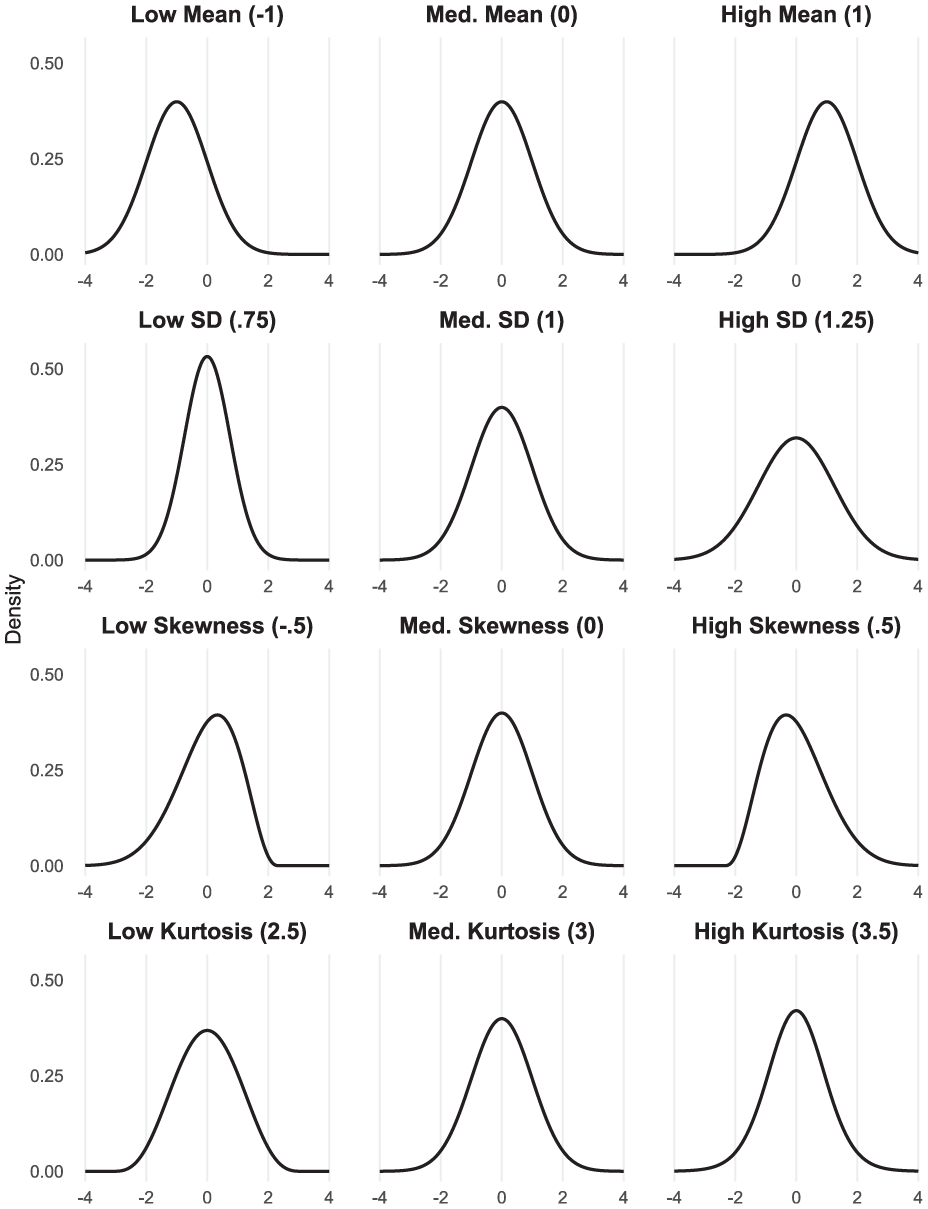
Low, Medium, and High Moment Values

Researchers often think about distributions in the context of descriptive statistics or assumption checks, only rarely considering how non-mean statistical moments of continuous predictor variables might explain binary criterion outcomes (for empirical examples in which they have, see Hehman et al., 2015; Sutherland et al., 2017; Todorov & Porter, 2014 for theoretical discussion, see Kane & Mertz, 2012). For binary criterion outcomes (or any discrete outcome, such as categorical outcomes, though we focus on binary outcomes for clarity), distribution moments such as variance and skewness play a vital role in explaining individuals’ and groups’ aggregate outcomes, as well as differences or disparities in these outcomes. Threshold models provide a simple way of understanding this.

Threshold Models

Threshold models broadly describe any model for which outcomes vary in some important way at specific values of the predictor (e.g., Fechner, 1966; Rouder & Morey, 2009; Toms & Lesperance, 2003; Vallacher & Nowak, 1994). These models have been used across the social and life sciences to describe various phenomena, such as group behavioral dynamics based on each individual’s threshold for engaging in a specific action (e.g., rioting; Granovetter, 1978); dose-response models describing at what dose a toxin begins to yield an effect or attains maximum effect (Calabrese & Baldwin, 2003); and recognition memory models in which items are either detected—yielding a correct information-based judgment—or not detected, yielding a guess (Kellen & Klauer, 2015).²

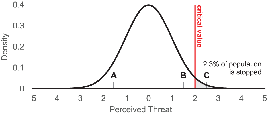
For our purposes, these models can explain how, for example, two people with relatively similar levels of a trait (e.g., the perceived threat of Persons B and C; Figure 2) can experience different outcomes (one is stopped by police, the other is not) and how two people with very different levels of a trait (e.g., the perceived threat of Persons A and B) can experience the same outcome (not being stopped by police). By solving for the integral of the population distribution beyond the threshold, threshold models can be used to calculate the proportion of outcomes in a given population.

Figure 2

Threshold Model Example

Hester et al. (2020) demonstrated how threshold models offer useful insights into the connection between stereotypes and discrimination. Intersectional patterns of discrimination (e.g., Black men being disproportionately stopped by police, relative to White men, Black women, and White women) can sometimes be explained by simple, non-intersectional stereotypes (e.g., Black people being perceived as more threatening than White people plus males being perceived as more threatening than females, without a unique interactive effect of being both Black and male). This work highlights the potential insights gained by thinking about stereotyping and discrimination—and attitudes and behaviors more broadly—using models that explicitly incorporate characteristics of the population distribution as predictors.

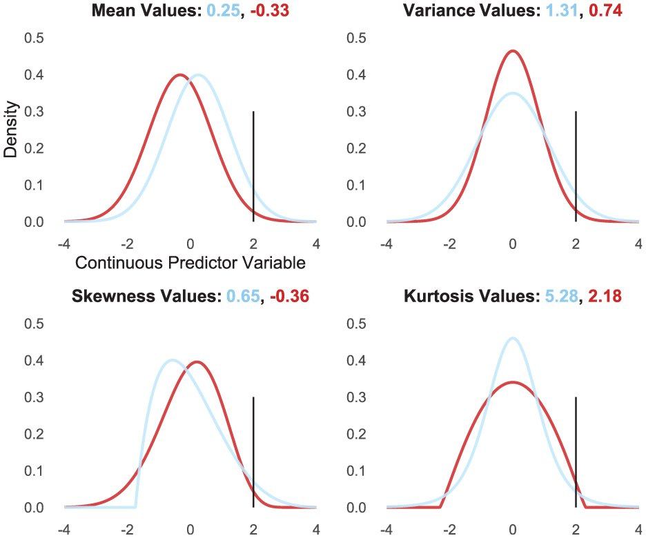
Figure 3 depicts two distributions representing two groups. Members of one group experience a critical outcome 4% of the time (light blue distribution) whereas members of the other group experience the same critical outcome 1% of the time (dark red distribution). For illustration, imagine that this binary criterion outcome is being stopped by a police officer (versus not being stopped). Although it might be most intuitive to explain the group gap in this outcome by positing a mean difference in perceived threat (i.e., the continuous predictor variable; top left panel), this gap might instead be accounted for by differences in other statistical moments—differences in variance (top right panel), skewness (bottom left panel), or kurtosis (bottom right panel). This observation resolves apparent inconsistencies where two groups show a disparity in binary outcomes despite possessing equal means in the underlying trait.

Figure 3

The Same Disparity in Binary Criterion Outcomes Explained by Different Distribution Moments

Importantly, the same insight translates to comparisons of individuals as well. Again in the context of Figure 3, imagine two individuals who each encounter police officers 100 times. One individual is stopped 4 times (4%; light blue distribution) and the other individual is stopped 1 time (1%; dark red distribution). The difference in these individuals’ critical outcomes might be explained by differences in mean, variance, skewness, kurtosis, or some combination of these distribution moments. The next section more closely examines the different types of distributions that can be relevant for understanding differences in binary criterion outcomes.

Relevant Distributions of Continuous Predictor Variables

Imagine a speed dating event at which 40 individuals—20 with tattoos and 20 without tattoos—each spend 5 minutes with the same 20 “potential partners,” half of whom are seeking casual relationships and half of whom are seeking serious relationships. For each of the 40 individuals, these potential partners indicate “Yes” or “No” in response to whether they would go on a first date (i.e., the binary criterion outcome). Underlying these decisions is perceived attraction (i.e., the continuous predictor variable).

Different distributions are relevant depending on the question. For the question “which individuals receive more yesses?,” target individual-level distributions of perceived attraction are relevant. For the question “do tattooed or non-tattooed individuals receive more yesses?,” target group-level distributions of perceived attraction are relevant. For the question “which potential partners give more yesses?,” rater individual-level distributions are relevant. Finally, for the question “do people seeking casual or serious relationships give more yesses?,” rater group-level distributions are relevant. Notably, the group-level questions resemble those typical in social psychology, where responses might be nested within both rater and target, with “Tattooed/Non-Tattooed” designated as a target-level predictor and “Casual/Serious” designated as a rater-level predictor in a cross-classified multilevel model. Conversely, individual-level questions more closely relate to questions concerned with prediction: for example, given an individual target’s distribution of perceived attraction, how many yesses would the model predict that they would receive?

Differences in mean, variance, skewness, and kurtosis exist for continuous variables. In the Supplemental Materials, we provide analyses describing moment differences for common trait judgments (target and rater individual-level distributions; target group-level distributions). We also describe moment differences for self-reported mental health, which would be relevant for modeling group differences in mental health–related diagnoses or behaviors.

Thus far, we have focused on the technical aspects of our argument and used only a couple specific examples as vehicles for explanation, which might raise the question: how broadly relevant and applicable are the core ideas presented? The next section highlights a few ways in which distribution moments are relevant to scientific inferences and methodological decisions.

Pitfalls in Scientific Reasoning

Forming accurate inferences from data is difficult. Using a means-focused approach to consider the relation between continuous predictor variables and binary criterion outcomes can result in intuitive but inaccurate inferences. We describe a few of these below.

Means-focused approaches can result in false negatives. For example, a researcher might posit that people who are perceived as attractive are more successful at arranging first dates. Imagine that this researcher finds that non-tattooed people are perceived as more attractive than tattooed people on average. However, they also find that the non-tattooed people and tattooed people successfully arrange first dates at equal rates. This researcher might interpret this pattern of findings as non-supportive of their hypothesis; however, it might be the case that their hypothesis is correct—attractive people are more likely to successfully arrange first dates—but that tattooed people showed higher variance and/or skewness in their perceived attractiveness than non-tattooed people, which caused the observed first date likelihood to be the same.

Alternately, imagine two target individuals who, across thousands of raters, have received the same mean attractiveness ratings. A predictive model that only accounts for mean differences would expect the same dating-related outcomes for both individuals: equal rates of success arranging first dates. However, to the extent that one of them has a higher variance and/or skewness in their distribution of attractiveness ratings, this individual would experience greater success arranging first dates (we analyze real data analogous to this example in Part II).

This last example is particularly relevant to stimulus selection: experimenters will often choose only one or a few stimuli per experimental condition, matching stimuli on relevant variables that might otherwise be confounded with condition (for a detailed review of stimulus sampling and new best practices, see Simonsohn et al., 2025; see also Wells & Windschitl, 1999). However, stimuli that are matched on mean levels of a relevant variable may still possess different distributions of that variable. If the experiment’s outcomes of interest are binary, the difference in distributions would constitute experimental confounds.

Means-focused approaches also create the potential for experimental effects to be solely attributed to a mean difference when the effect is accounted for by both mean and non-mean moments of the continuous predictor variable. For example, the effectiveness of an experimental manipulation might be verified in a pilot study or by using direct manipulation checks included in the experiment itself. It is common practice to test for a mean difference on a manipulation check item, and, if this test is statistically significant, to claim that the manipulation was effective (e.g., in Ejelöv & Luke, 2020, 88/134 papers reporting direct manipulation checks included a statement of effectiveness). Any subsequent effects of such an experimental manipulation on binary outcomes would be interpreted as caused by the underlying mean difference in the manipulated internal state. Even if the general attribution of the binary outcome to the internal state is correct, evaluations of causal efficacy will be skewed (e.g., concluding that the ratio of cause size to effect size is small when the manipulation also created differences in the variance of the operationalized continuous predictor variable; Abelson, 1995; Ejelöv & Luke, 2020).

This list of potential pitfalls is not exhaustive, but justifies the present research, which aims to clarify the relation between continuous predictor variables and binary criterion outcomes. In doing so, we hope to equip researchers to better avoid these pitfalls and to pursue additional hypothesis testing focused on non-mean moments.

Present Research

We consider the extent to which differences in the distribution moments of continuous predictor variables translate to differences in binary criterion outcomes (Part I). Then, we show that modeling non-mean moments can produce different predicted patterns of binary criterion outcomes (Part II). Finally, we provide an example of how distribution moments can help clarify existing work, using gender differences in risk-taking as an example (Part III).

Open Data and Materials

All data and materials are available at https://osf.io/8dahg, including HTML Markdowns for all analyses. We did not preregister our studies or conduct power analyses.

Part I: Modeling the Extent to Which Differences in Distribution Moments Translate to Disparities in Binary Criterion Outcomes

We simulated data for Group A and Group B to estimate how differences between moments of the continuous predictor variable translate into differences in binary criterion outcomes. We modeled the relation between these variables using threshold models. The position of the threshold ranged from −3 to 3 (the j loop; 61 iterations with threshold value ranging from 3 to −3 at .1 intervals). Both groups started with a standardized normal distribution (M = 0, variance = 1, skewness = 0, kurtosis = 3), which resulted in the same proportion of binary outcomes for each group. Then, we gradually increased group differences for each moment (holding other moments constant) using the PearsonDS package (Becker & Klößner, 2017). The difference between Group A and Group B for each moment was increased by .1 units in each iteration, up to .5 units, with the exception of the mean, for which differences were increased by .2 units in each iteration up to 1 (the k loop; note that mean differences between groups are typically larger than differences in other moments). Note that .1 iterations were applied to the standard deviation (the square root of the variance) rather than the variance, as researchers typically describe variance using standard deviation.This k loop thus had six iterations per moment, resulting in 61 (j) × 6 (k) = 366 iterations per moment. These differences were created by “spreading” the moment values for each group equally from their starting points. For example, for a skewness difference of .2, Group A has a skewness of −.1 and Group B has a skewness of .1. See the markdown for full documentation of the method.

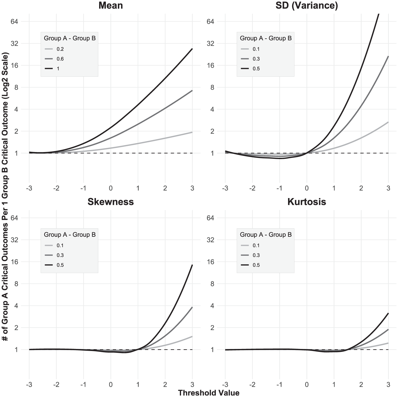
Figure 4 displays the results. We avoid making direct comparisons between moments because unit magnitude is not equivalent across moments. For critical outcomes with lower thresholds (e.g., −2), differences in all moments hardly impact the ratio of Group A to Group B outcomes, because receiving the outcome is so common. For example, at a threshold of −2 and a mean difference of 1, members of Group A experience an outcome 99.38% of the time and members of Group B experience an outcome 93.33% of the time, such that 1.06 members of Group A experience the outcome per one member of Group B.

Figure 4

Relative Differences in Critical Outcomes as a Function of Threshold and Group Differences in Moments

For critical outcomes with medium thresholds (e.g., 0), differences in mean impact the ratio between Group A and Group B outcomes, whereas differences in other moments do not. However, for critical outcomes with higher thresholds (e.g., 2), differences in variance and skewness both clearly impact the ratio of Group A to Group B outcomes and scale considerably as group differences in these moments increase (note that the y-axis is on a log2 scale to promote the readability of the curves). For example, at a threshold of 2 and a standard deviation difference of .5, members of Group A experience an outcome 5.48% of the time and members of the other group experience an outcome 0.38% of the time, such that 14.42 members of Group A experience the outcome per one member of Group B. Note that effect of group differences in mean on critical outcome ratios also increases at higher thresholds, but with less pronounced scaling. Differences in kurtosis have little effect on target outcome disparities, except at very high thresholds.

In the Supplemental Materials, we have provided additional simulations that vary two moments at once. Although a full discussion of these simulations is beyond the scope of the manuscript, we generally find that group differences in one moment (e.g., a higher mean for Group A compared with Group B) show amplified effects on outcome ratios when another moment is also higher (e.g., a higher SD for Group A compared with Group B).

Part I Discussion

Part I examined the extent to which differences in moments for the continuous predictor variable translate to differences in the binary criterion outcome. Holding other moments constant, differences in variance and skewness can result in substantial differences in outcomes, with kurtosis showing more modest effects. For example, at a threshold value of 2, a .4-unit difference in standard deviation between targets results in the high-SD target experiencing the outcome (e.g., getting a first date) 8 times as often as the low-SD target, despite the two targets having identical mean values.

Unfortunately, there is no clear standard for what a “small” or “large” difference in variance, skewness, or kurtosis is—as such, it is hard to understand exactly how important each moment is for predicting differences in binary criterion outcomes. However, it appears to roughly be the case that the “impact” of each moment declines with each increase in order, such that mean differences in continuous predictor variables are most important, followed by variance differences, then skewness and kurtosis differences. Part II moves from simulation to real data to demonstrate how modeling non-mean moments for continuous predictor variables produces meaningful differences in binary criterion outcomes.

Part II: Including Non-Mean Moments Changes Predicted Outcomes

Some individuals have more “polarizing” appearances than others. For example, Christian Rudder (2014) used data from the dating website OkCupid to show that, holding mean profile rating constant,³ people with higher variance in profile ratings received more messages.

Figure 5 compares two Black men from the Chicago Face Database (Ma et al., 2015) with nearly equivalent mean attractiveness ratings (and nearly equivalent kurtoses) from 11,484 raters (Jones et al., 2021). However, Target A has a lower SD (1.72) and skewness (.28) than Target B, who has a higher SD (1.91) and skewness (.47). Without incorporating distribution moments, we would predict that these men would have equal success going on first dates. However, when both men’s full distributions of attractiveness ratings are modeled with a threshold of 7 determining “first date success,” we would predict that Target A would only have a success rate of 3.76% compared with Target B’s success rate of 6.28%.

Figure 5

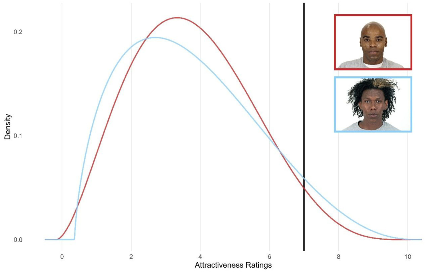
First Date Threshold Model for Two Black Male Targets

Part II Discussion

We illustrated how the predicted pattern of binary criterion outcomes changes when non-mean moments are modeled. To do this, we focused on two targets with nearly identical mean levels of attractiveness but different variances and skewnesses. This example is particularly relevant to experimental stimulus sampling, where matching stimuli on relevant variables is common practice. When experimental outcomes of interest are binary, simply matching stimuli based on means may not be enough to de-confound experimental conditions.

Part III: Illustration Using ExtremeRisk-Taking and Distribution Moments

In Part III, we provide a concrete illustration of how insights from the present work can hone researchers’ reasoning about data. We show how an abductive inferential approach (i.e., attempting to find a feasible causal explanation for observed phenomena) that accounts for all moments yields useful predictions about gender differences in risk-taking propensity distributions, which might help explain large gender differences in extreme risk-taking behavior.

Risk-Taking Propensity and Gender

Research indicates that men, on average, take more risks than women. The size of this gender difference varies by context: a meta-analysis (Byrnes et al., 1999) found that mean standardized gender effects are quite small for self-reported activities such as smoking (-.02), drinking and drug use (.04), and sexual activity (.07), but larger for driving (.29) and other activities (.38). For behaviors observed in a lab setting, the researchers found more modest effect sizes in driving (.17) and gambling (.21) tasks. Between this and other research finding modest gender differences in sensation-seeking (Cross et al., 2013) and impulsivity (Cross et al., 2011), one might conclude that, although there are gender differences in sensation seeking, they are small.

However, this research appears to be misaligned with observed extreme risk-taking in the real world. For example, if gender differences in risk-taking are small, why is it the case that 94% of deaths from BASE jumping⁴ are men (BASE Addict, 2024)? From this perspective, such large differences in these more extreme risks seem surprising. There might, of course, be other gender differences that account for this—BASE jumping safety might depend on height or weight, which differs by sex, or women may simply be better BASE jumpers. However, risk-taking propensity seems like a reasonable predictor of this particular outcome, and we focus on it for the present argument.

A researcher taking an abductive approach might start with these observed phenomena (in BASE jumping, 18 men dying per one woman) and search for differences in risk-taking propensity. Means-focused approaches would posit a very large effect size for mean gender differences, but the small effect sizes evident in the meta-analyses are inconsistent with this interpretation: these small mean effect sizes cannot account for the large observed differences in deaths. On the other hand, accounting for all distribution moments might additionally allow predictions that there are gender differences in variance and/or skewness that help account for the large gender gaps in extreme risk-taking behaviors.

We examined responses on a risk-taking propensity scale, predicting that there would be gender differences in variance, skewness, and/or kurtosis in addition to mean gender differences, both in general risk-taking and in recreational risk-taking specifically. Then, we fit a model predicting extreme risk-taking with risk-taking propensity scores, comparing models that incorporate and do not incorporate gender differences in variance, skewness, and kurtosis.

Method

We examined 3123 responses (50% women, M_age = 36 years) to the DOmain-SPEcific Risk-Taking scale (DOSPERT; Blais & Weber, 2006) taken from a study conducted by Frey and colleagues (2020). Following this work, we fit a bifactor model using the lavaan package in R (Rosseel, 2012) to estimate both a general risk-taking factor and five specific subfactors in these domains: ethical, financial, health-related, recreational, and social. We estimated standardized latent factor scores for each respondent, then used the same bootstrapping procedure used in Part II to estimate means, variances, skewnesses, and kurtoses for men and women in the sample.

Results

Keeping in mind the abductive approach used in this example—trying to find a reasonable explanation for the 18:1 ratio of men:women who die BASE jumping—we expected not only mean gender differences in risk-taking, but also potential differences in variance and skewness. Figure 6 shows the results.

Figure 6

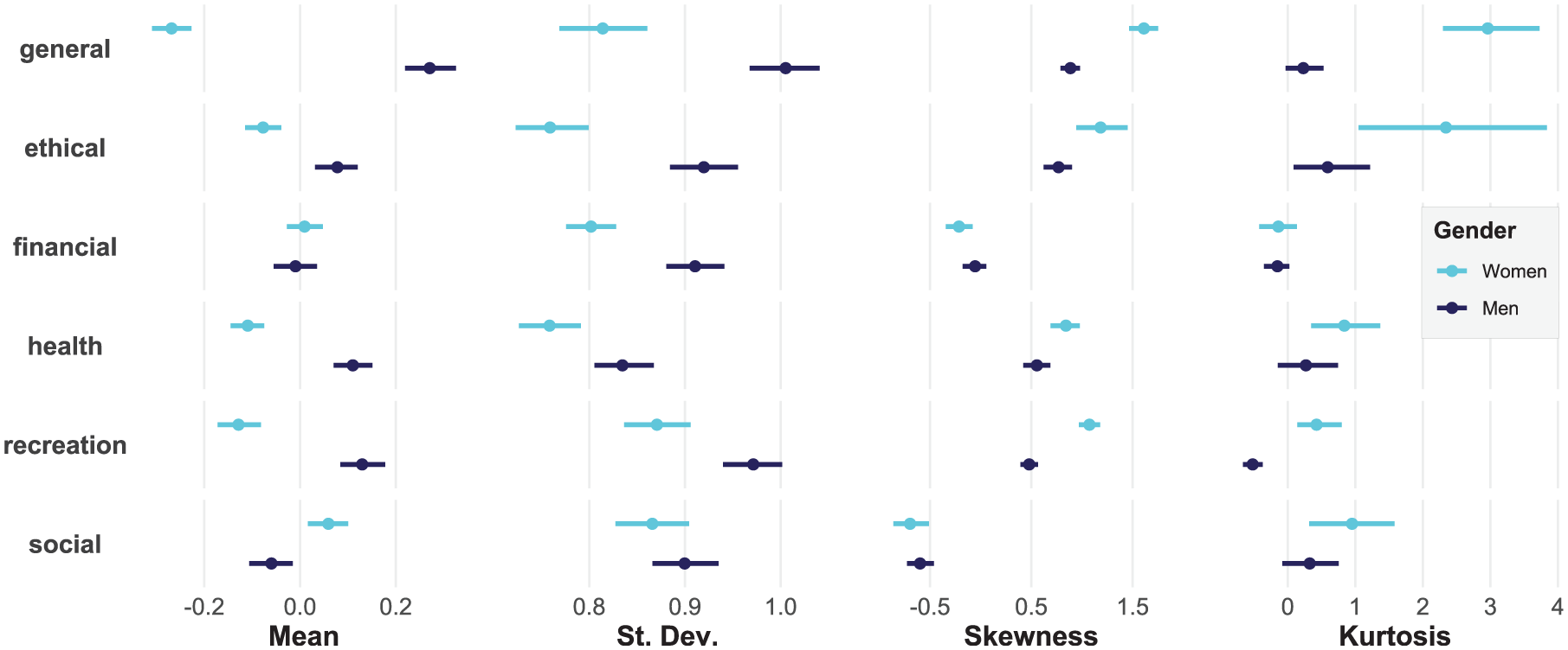
Moments by Gender for Domain-Specific Risk-Taking Scores, General and Subscales

Men scored higher than women for most kinds of risk-taking, such that there was a medium-large gender effect for general risk-taking (Cohen’s d = .59) as well as small-medium gender effects for recreational (d = .28), ethical(d = .18), and health (d = .27) risk-taking. For social risk-taking, mean scores were higher for women than for men (d = .13). The effect size for recreational risk-taking, though robust, does not appear large enough to account for the large observed differences in BASE jumping deaths. To this end, we also found differences in standard deviation for both general (SD_{men - women} = .19) and recreational (SD_{men – women} = .10) risk-taking, matching expectations from our abductive approach. Although a .1 difference in SD for recreational risk-taking might seem small, this difference likely has a sizable effect on extreme critical outcomes in the context of the mean difference that we also observed.⁵

Finally, we also note differences in skewness and kurtosis for general and recreational risk-taking, such that women are higher in both compared with men. All else equal, these differences would predict that women are more likely to engage in risky activities in these domains; however, in concert with mean and variance differences, men should still engage in extreme risky behaviors more often than women. Raw density plots clarify this point (Figure 7).

Figure 7

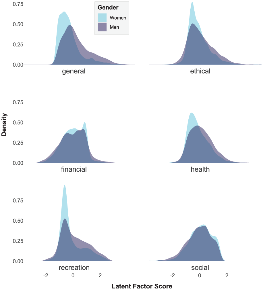
Density Plots by Gender for Domain-Specific Risk-Taking Scores, General and Subscales

As a final illustration, we estimated the threshold that would predict an 18:1 ratio in male to female deaths for BASE jumping, using a Pearson distribution defining risk propensity distributions for both men and women. The threshold that produced this 18:1 ratio was 3.07. Then, we applied this threshold to a means-only model that assumes equal variance, skewness, and kurtosis across men and women (in this case, a static value that is the average of the observed moment values for men and women). This means-only model estimated a 6.5:1 ratio in male to female deaths, rather than an 18:1 ratio.⁶

Part III Discussion

Part III illustrates the benefits of modeling moments for scientific inference. By recognizing the potential role of variance in risk-taking propensity for explaining large observed gender disparities in extreme outcomes, we improved our abductive reasoning by considering gender differences in variance as one potential explanation for these gender disparities. Furthermore, we demonstrated that modeling the ratio of male-to-female BASE jumping deaths with versus without non-mean moments produced a substantial difference in the predicted ratio.

General Discussion

Using simulations, we demonstrated that differences in the non-mean distribution moments of continuous predictor variables (e.g., perceived threat) can translate to substantial differences in binary criterion outcomes (e.g., police stops; Part I). Then, using face perception data, we compared the distribution of attractiveness ratings of two individuals with nearly equivalent means but different variances and skewnesses and illustrated how individuals with higher variance and more right-skewed ratings might experience more positive outcomes (Part II). Finally, we showed how insights from this paper can improve existing psychological theory, using large gender differences in extreme risk-taking behavior to predict the existence of gender differences in the variance of risk-taking propensity (Part III).

The goal of this paper is to highlight how and to what extent distribution moments are relevant to scientific reasoning and common research practices. We certainly do not argue that these moments-based explanations are novel; certainly, researchers have posited group differences in variance and skewness as explanations for group differences in outcomes across various domains. Perhaps most famously, the variability hypothesis argues that biological characteristics cause males to show greater population variability than females for myriad physical and mental traits, explaining their overrepresentation in domains ranging from mental asylums to genius societies (see Shields, 1982 for historical context; Thöni & Volk, 2021). This hypothesis has been used by some researchers to posit that STEM gender disparities in binary outcomes (e.g., prestigious awards and positions) are because of biological gender differences in aptitude variability rather than average aptitude (Johnson et al., 2008; for rebuttal, see Hyde & Mertz, 2009; Kane & Mertz, 2012).

Limitations and Future Directions

Although the methodology employed in the present research is well-suited for our basic questions, there are limitations of the threshold model framework. First, the models used are specifically designed for binary outcomes and do not produce standard inferential test statistics or effect size estimation. The tools that we used are well-suited for a proof-of-concept investigation, but future quantitative developments are needed to better equip researchers for testing hypotheses involving effects of non-mean moments. There is, of course, an enormous body of literature documenting approaches to predicting binary outcomes using continuous predictors, primary among these being logistic regression (Weisberg, 2005; Wong & Mason, 1985; Wright, 1995). However, little guidance and few tools exist for incorporating statistical moments as predictors of outcomes. Although creating formal statistical modeling tools is beyond the scope of this article, these tools would expand the impact of the present work.

Furthermore, here we assume that threshold positions do not vary across groups or individuals, but this is sometimes the case. For example, women may need to be “better” than men to receive the same promotion (status characteristics theory; Berger et al., 1980), or men might need to do more than women to be fired (shifting standards model; Biernat & Kobrynowicz, 1997; Biernat & Manis, 1994). Shifting thresholds do not undermine the arguments in this paper, but they are important to note, and future work might simultaneously examine group differences in distribution shape and threshold position.

Conclusion

A central goal of psychological research is to form accurate inferences about associations between continuous predictor variables and binary criterion outcomes. In some cases, this goal would be better achieved by considering individual or group differences in the full distribution of continuous predictor variables, rather than mean differences alone. Variance, skewness, and kurtosis (from most to least important) may play a key role in explaining disparities between individuals and groups for life-changing outcomes such as being arrested by the police, participating in high-risk recreational activities, landing a sought-after job, or embarking on a first date with one’s future partner. Such distribution differences may be more common than their presence in the research literature suggests. For example, as discussed, manipulation checks for experimental conditions rarely consider non-mean differences. By closely examining the relation between continuous predictor variables and binary criterion outcomes, we hope to equip researchers to make more accurate inferences about their data, which will in turn yield more accurate models for understanding the psychological predictors of some of the most important events and behaviors in people’s lives.

Supplemental Material

sj-docx-1-spp-10.1177_19485506251385636 – Supplemental material for Differences in Variance, Skewness, and Kurtosis Can Account for Differencesin Binary Outcomes

Supplemental material, sj-docx-1-spp-10.1177_19485506251385636 for Differences in Variance, Skewness, and Kurtosis Can Account for Differencesin Binary Outcomes by Neil Hester and Eric Hehman in Social Psychological and Personality Science

Footnotes

Acknowledgements

We have no acknowledgments.

Handling Editor: Unkelbach Christian

Author Contributions

Conceived research: N.H. Methodology: All authors. Investigation: All authors. Analysis and visualization: N.H. Writing—Original Draft: N.H. Writing—Review and Editing: All authors.

Declaration of Conflicting Interests

The authors declared no potential conflicts of interest with respect to the research, authorship, and/or publication of this article.

Funding

The authors received no financial support for the research, authorship, and/or publication of this article.

ORCID iDs

Neil Hester

Eric Hehman

Data Availability Statement

Data and code for main and supplemental analyses are available at .

Supplemental Material

Supplemental material is available in the online version of the article at .

Notes

Author Biographies

Neil Hester investigates the myriad factors that explain how perceivers form impressions of targets. This work encompasses topics such as stereotyping and discrimination, perceptions of bodies and clothing, face perception, social categorization, and social cognition more broadly. He also grapples with issues of measurement and causal inference, particularly in the domain of person perception.

Eric Hehman investigates the causes and consequences of intergroup prejudices, and how perceptions across group boundaries (e.g., race, gender, sexual-orientation, occupation, etc) contribute to intergroup dynamics. To address these questions, he takes a multi-method approach, incorporating a broad range of behavioral (e.g., computer-mouse tracking, digital face modeling, group interactions) and statistical techniques (e.g., multilevel modeling, structural equation modeling, machine learning).

References

Abelson

R. P.

(1995). Statistics as principled argument. Lawrence Erlbaum. https://doi.org/10.4324/9781410601155

BASE Addict. (2024). BASE jumping fatalities—Analytics. https://bfl.baseaddict.com/analytics.

Becker

Klößner

(2017). Package “PearsonDS.” https://doi.org/10.32614/CRAN.package.PearsonDS

Berger

Rosenholtz

S. J.

Zelditch

(1980). Status organizing processes. Annual Review of Sociology, 6, 479–508. https://doi.org/10.1146/annurev.so.06.080180.002403

Biernat

Kobrynowicz

(1997). Gender- and race-based standards of competence: Lower minimum standards but higher ability standards for devalued groups. Journal of Personality and Social Psychology, 72(3), 544–557. https://doi.org/10.1037/0022-3514.72.3.544

Biernat

Manis

(1994). Shifting standards and stereotype-based judgments. Journal of Personality and Social Psychology, 66(1), 5–20. https://doi.org/10.1037//0022-3514.66.1.5

Blais

A.-R.

Weber

(2006). A Domain-Specific Risk-Taking (DOSPERT) scale for adult populations. Judgment and Decision Making, 1, 33–47. https://doi.org/10.1037/t13084-000

Byrnes

Miller

Schafer

(1999). Gender differences in risk taking: A meta-analysis. Psychological Bulletin, 125, 367–383. https://doi.org/10.1037//0033-2909.125.3.367

Calabrese

E. J.

Baldwin

L. A.

(2003). Hormesis: The dose-response revolution. Annual Review of Pharmacology and Toxicology, 43(1), 175–197. https://doi.org/10.1146/annurev.pharmtox.43.100901.140223

10.

Cross

C. P.

Copping

L. T.

Campbell

(2011). Sex differences in impulsivity: A meta-analysis. Psychological Bulletin, 137(1), 97–130. https://doi.org/10.1037/a0021591

11.

Cross

C. P.

Cyrenne

D.-L. M.

Brown

G. R.

(2013). Sex differences in sensation-seeking: A meta-analysis. Scientific Reports, 3(1), 2486. https://doi.org/10.1038/srep02486

12.

Ejelöv

Luke

T. J.

(2020). “Rarely safe to assume”: Evaluating the use and interpretation of manipulation checks in experimental social psychology. Journal of Experimental Social Psychology, 87, 103937. https://doi.org/10.1016/j.jesp.2019.103937

13.

Fechner

G. T.

(1966). Elements of psychophysics. Holt, Rinehart & Winston. https://doi.org/10.1037/11304-026

14.

Frey

Duncan

Weber

E. U.

(2020). Towards a typology of risk preference: Four risk profiles describe two thirds of individuals in a large sample of the U.S. population. PsyArXiv. https://doi.org/10.31234/osf.io/yjwr9

15.

Granovetter

(1978). Threshold models of collective behavior. American Journal of Sociology, 83(6), 1420–1443. https://doi.org/10.1086/226707

16.

Hehman

Flake

J. K.

Freeman

J. B.

(2015). Static and dynamic facial cues differentially affect the consistency of social evaluations. Personality and Social Psychology Bulletin, 41(8), 1123–1134. https://doi.org/10.1177/0146167215591495

17.

Hester

Payne

Brown-Iannuzzi

Gray

(2020). On intersectionality: How complex patterns of discrimination can emerge from simple stereotypes. Psychological Science, 31(8), 1013–1024. https://doi.org/10.1177/0956797620929979

18.

Hyde

J. S.

Mertz

J. E.

(2009). Gender, culture, and mathematics performance. Proceedings of the National Academy of Sciences, 106(22), 8801–8807. https://doi.org/10.1073/pnas.0901265106

19.

John

Angelov

Öncül

A. A.

Thévenin

(2007). Techniques for the reconstruction of a distribution from a finite number of its moments. Chemical Engineering Science, 62(11), 2890–2904. https://doi.org/10.1016/j.ces.2007.02.041

20.

Johnson

Carothers

Deary

I. J.

(2008). Sex differences in variability in general intelligence: A new look at the old question. Perspectives on Psychological Science, 3(6), 518–531. https://doi.org/10.1111/j.1745-6924.2008.00096.x

21.

Jones

B. C.

DeBruine

L. M.

Flake

J. K.

Liuzza

M. T.

Antfolk

Arinze

N. C.

Ndukaihe

I. L. G.

Bloxsom

N. G.

Lewis

S. C.

Foroni

Willis

M. L.

Cubillas

C. P.

Vadillo

M. A.

Turiegano

Gilead

Simchon

Saribay

S. A.

Owsley

N. C.

Jang

. . .Coles

N. A.

(2021). To which world regions does the valence–dominance model of social perception apply? Nature Human Behaviour, 5(1), 159–169. https://doi.org/10.1038/s41562-020-01007-2

22.

Kane

J. M.

Mertz

J. E.

(2012). Debunking myths about gender and mathematics performance. Notices of the American Mathematical Society, 59(01), 10. https://doi.org/10.1090/noti790

23.

Kellen

Klauer

K. C.

(2015). Signal detection and threshold modeling of confidence-rating ROCs: A critical test with minimal assumptions. Psychological Review, 122(3), 542–557. https://doi.org/10.1037/a0039251

24.

D. S.

Correll

Wittenbrink

(2015). The Chicago face database: A free stimulus set of faces and norming data. Behavior Research Methods, 47(4), 1122–1135. https://doi.org/10.3758/s13428-014-0532-5

25.

Pearson

Henrici

O. M. F. E.

(1894). III. Contributions to the mathematical theory of evolution. Philosophical Transactions of the Royal Society of London A, 185, 71–110. https://doi.org/10.1098/rsta.1894.0003

26.

Rosseel

(2012). Lavaan: An R package for structural equation modeling and more. Version 0.5—12 (BETA). Journal of Statistical Software, 48(2), 1–36. https://doi.org/10.18637/jss.v048.i02

27.

Rouder

J. N.

Morey

R. D.

(2009). The nature of psychological thresholds. Psychological Review, 116(3), 655–660. https://doi.org/10.1037/a0016413

28.

Rudder

(2014). Dataclysm: Who we are (when we think no one’s looking). Random House Canada. https://dl.acm.org/doi/abs/10.5555/2677103

29.

Shields

S. A.

(1982). The variability hypothesis: The history of a biological model of sex differences in intelligence. Signs: Journal of Women in Culture and Society, 7(4), 769–797. https://doi.org/10.1086/493921

30.

Simonsohn

Montealegre

Evangelidis

(2025). Stimulus sampling reimagined: Designing experiments with mix-and-match, analyzing results with stimulus plots. Journal of Personality and Social Psychology, 129(1), 71–90. https://doi.org/10.1037/pspa0000449

31.

Sutherland

C. A. M.

Young

A. W.

Rhodes

(2017). Facial first impressions from another angle: How social judgements are influenced by changeable and invariant facial properties. British Journal of Psychology, 108(2), 397–415. https://doi.org/10.1111/bjop.12206

32.

Thöni

Volk

(2021). Converging evidence for greater male variability in time, risk, and social preferences. Proceedings of the National Academy of Sciences, 118(23), e2026112118. https://doi.org/10.1073/pnas.2026112118

33.

Todorov

Porter

J. M.

(2014). Misleading first impressions: Different for different facial images of the same person. Psychological Science, 25(7), 1404–1417. https://doi.org/10.1177/0956797614532474

34.

Toms

J. D.

Lesperance

M. L.

(2003). Piecewise regression: A tool for identifying ecological thresholds. Ecology, 84(8), 2034–2041. https://doi.org/10.1890/02-0472

35.

Vallacher

R. R.

Nowak

A. E.

(1994). Dynamical systems in social psychology. Academic Press. https://doi.org/10.1126/science.265.5174.977

36.

Weisberg

(2005). Applied linear regression (Vol. 528). John Wiley. https://doi.org/10.1002/0471704091

37.

Wells

G. L.

Windschitl

P. D.

(1999). Stimulus sampling and social psychological experimentation. Personality and Social Psychology Bulletin, 25(9), 1115–1125. https://doi.org/10.1177/01461672992512005

38.

Wong

G. Y.

Mason

W. M.

(1985). The hierarchical logistic regression model for multilevel analysis. Journal of the American Statistical Association, 80(391), 513–524. https://doi.org/10.1080/01621459.1985.10478148

39.

Wright

R. E.

(1995). Logistic regression. In Reading and understanding multivariate statistics (pp. 217–244). American Psychological Association.

Supplementary Material

Please find the following supplemental material available below.

For Open Access articles published under a Creative Commons License, all supplemental material carries the same license as the article it is associated with.

For non-Open Access articles published, all supplemental material carries a non-exclusive license, and permission requests for re-use of supplemental material or any part of supplemental material shall be sent directly to the copyright owner as specified in the copyright notice associated with the article.

0.00 MB

11.63 MB

Differences in Variance,Skewness,and Kurtosis Can Account for Differences in Binary Outcomes

Abstract

Keywords

Statistical Moments About the Mean

Threshold Models

Relevant Distributions of Continuous Predictor Variables

Pitfalls in Scientific Reasoning

Present Research

Open Data and Materials

Part I: Modeling the Extent to Which Differences in Distribution Moments Translate to Disparities in Binary Criterion Outcomes

Part I Discussion

Part II: Including Non-Mean Moments Changes Predicted Outcomes

Part II Discussion

Part III: Illustration Using ExtremeRisk-Taking and Distribution Moments

Risk-Taking Propensity and Gender

Method

Results

Part III Discussion

General Discussion

Limitations and Future Directions

Conclusion

Supplemental Material

sj-docx-1-spp-10.1177_19485506251385636 – Supplemental material for Differences in Variance, Skewness, and Kurtosis Can Account for Differencesin Binary Outcomes

Footnotes

Acknowledgements

Author Contributions

Declaration of Conflicting Interests

Funding

ORCID iDs

Data Availability Statement

Supplemental Material

Notes

Author Biographies

References

Supplementary Material