No Evidence of a Gender-Equality Paradox in Gendered Names: Comment on Vishkin,Slepian,and Galinsky (2022)

Abstract

This article reexamines the results of Vishkin, Slepian, and Galinsky (2022), which found larger gender differences in voiced names with higher gender equality over time and across states. I show that the employed statistical methods and calculations led the authors to draw incorrect conclusions. Using more appropriate methods, I show that there is no evidence of a systematic decrease in the proportion of voiced female names over time nor a corresponding increase for male names in Study 1 and that the gender difference has actually decreased. In Study 2, I show that, contrary to the authors’ hypothesis, both men and women have a higher proportion of voiced names in states with higher female leadership scores and that the increased difference disappears when controlling for a cultural confound—states’ proportion of foreign-born inhabitants. I conclude by discussing some overarching issues and thoughts on best practices.

The gender-equality paradox refers to the result that countries with higher gender equality have shown larger gender differences on different psychological measures (e.g., Falk & Hermle, 2018; Mac Giolla & Kajonius, 2019; Schmitt et al., 2008), and the occasional behavioral outcome (Stoet & Geary, 2018; Vishkin, 2022). These correlational results are commonly given a causal interpretation by the authors—that higher gender equality leads to increased gender differentiation, either due to an increased expression of innate gender-specific preferences (e.g., Falk & Hermle, 2018) or, as in Vishkin et al. (2022), due to a reactive preference for optimal distinctiveness between genders—a motivation to make men appear more masculine and women more feminine as a result of a decreased differentiation on other dimensions (e.g., political equality).

In Vishkin et al. (2022), the authors’ gender-equality paradox outcome of choice is the proportion of “voiced” and “unvoiced” names given to baby boys and girls. Voiced names are, according to the authors’ classification, names that begin with A, B, D, E, G, I, J, L, M, N, O, R, U, V, W, X, Y, or Z, which are said to sound harder and more stereotypically masculine. Unvoiced names instead begin with C, F, H, K, P, Q, S, or T and are said to sound softer and more stereotypically feminine. The authors therefore take an increased proportion of voiced names given to boys and a decrease for girls as a reflection of parents’ preferences for gender differentiation, which, by the authors’ explanation for the gender-equality paradox, is believed to increase with greater gender equality. The authors present two studies to support this hypothesis.

In Study 1, the authors use multilevel regression with intercepts for years as random factors to assess variation in the proportion of voiced names for boys and girls over a time period of increasing gender equality. Gender is treated as a Level 1 variable and year as a Level 2 variable. Differentiation is assessed with the Gender × Year interaction. Two samples are used: one for the United States between the years 1880 and 2018 and one for England and Wales over 10-year intervals between the years 1904 and 1994. In both cases, using linear and logistic regression respectively, the authors find an overall negative slope for the proportion of voiced names given to girls and a significant difference to the slope for boys, which was slightly positive instead (significantly and non-significantly, respectively).

In Study 2, the authors use linear multilevel regression across U.S. states in the year 2018 with state-level intercepts as random factors. Gender is treated as a Level 1 variable and state as a Level 2 variable. States were ranked by gender equality and female leadership. The authors did not find a significant overall Gender Equality × Gender interaction on the proportion of voiced names but did so for the Female Leadership × Gender interaction. The proportion of voiced names was higher for both boys and girls in states with higher female leadership scores, but the increase compared to states with low female leadership scores was higher for boys than for girls.

Clarifying the Authors’ Hypothesis

The authors do not quite make it clear in the article what they consider to corroborate versus to refute their hypothesis about optimal distinctiveness, but from comments from one author, ¹ it appears they consider it corroborated if the following three things are fulfilled: (1) There is a significant association between gender equality and the proportion of voiced names in the right direction for at least one gender (higher proportion for boys and lower for girls), (2) the trend in this direction is stronger for the correct gender than for the other (significant interaction), and (3) the association for the other gender is not significantly in the wrong direction (lower proportion for boys and higher for girls). The last point means that both proportions do not change significantly in the same direction, as this would mean that both genders, for example, are increasingly given masculine attributes.

These predictions mean that even if higher gender equality results in smaller differences, this can still be considered support for the authors’ hypothesis, provided the proportions are in the “wrong” direction with lower gender equality. This is problematic however, because if there is a smaller difference, then it is difficult to argue that a paradox exists at all: This is exactly what to expect if gender equality causes parents to name boys and girls as equally as possible, with the common proportion of voiced names lying in-between the previous male and female proportions. That would, for example, happen if parents gender-neutrally selected their favorites from the names around them and then adapted those names to a male or female version (e.g., they like Carla, so they name their boy Carl). Consequently, I will consider the results both from the authors’ perspective and by assessing the difference between genders, as a smaller difference opens up alternative explanations like the one above. Even with tests ignoring the difference, however, there appears to be little evidence for the authors’ hypothesis.

Reevaluating Study 1

The usual multilevel method for assessing trends over time is to treat subjects as a Level 2 variable and time as a Level 1 variable (e.g., Section 1.2 in the authors’ reference about fitting multilevel models; Bates et al., 2015). As the authors only have one subject in each analysis (the United States in one case and England and Wales in the other), time is instead used as a Level 2 variable. In multilevel models with random effects, the different Level 2 subjects are considered independent random draws from a population of possible subjects, and overall effects are calculated based on the estimated average effect over that population (see, e.g., Sections 1.1 and 2.2 in Bates et al., 2015). However, timepoints are not independent randomly drawn subjects, as the outcome for one timepoint will (at least) depend on the outcome of the previous timepoint. Consequently, treating time as Level 2 subjects is problematic, as the increased dependence will increase the covariation between neighboring timepoints and skew the inference statistics. See Figure 1 for an illustration.

Figure 1

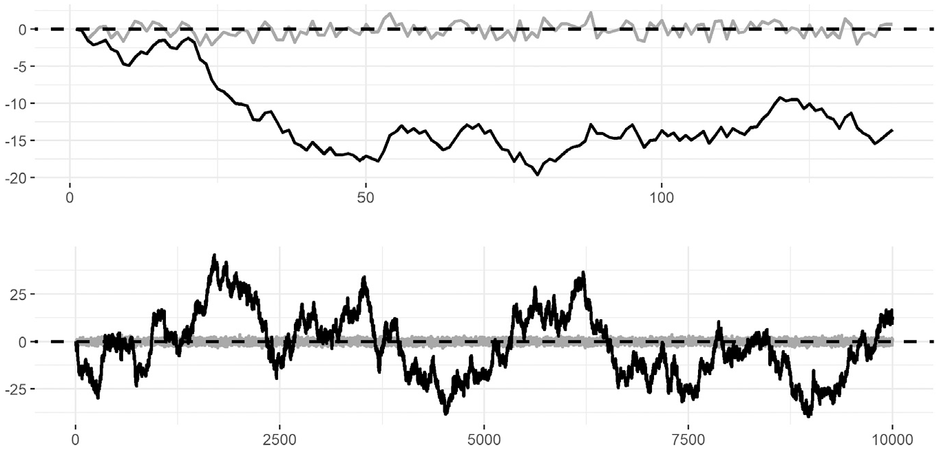
Illustration of How Time Series Data Compare to Independent Data When There Is No Systematic Pattern Over Time, for 139 Years at the Top (Same Range as the U.S. Data) and 10⁴ Years at the Bottom

Simulation of Error Rates

How problematic is the above for the authors’ conclusions? For inferential statistics to be valid, the p values would need to reflect (at least approximately) how often a result of at least the observed magnitude is found if the null-hypothesis of no effect in the population is true. That is, if an observed effect corresponds to a p value of say .05 and if there is no effect in the population, then observations of at least the observed magnitude should only happen in about .05 of all samples. Thus, for the authors’ method to work as intended, dependence between datapoints should not increase those proportions too far above .05. To examine whether this holds true, I used R v.4.0.1 to simulate 10⁴ observations either from two independent series or two time series with dependent timepoints. In both cases, there was no trend over time nor any systematic interaction between the series (i.e., the null-hypothesis of no effects held). The results of these simulations showed that estimating the significance for the interaction term with the authors’ multilevel model worked well for the independent series, this being significant in .057 of simulated samples (close to the alpha level of .05). However, when there was dependence between datapoints (as for timepoints), this proportion increased dramatically to .900. Similarly, although the high t values found by the authors would all correspond to ps < .001 in an independent series, introducing dependence between datapoints resulted in t values at least as high as the authors’ gender, year, and Gender × Year t values (4.64, 9.81, and 15.34, respectively) to be found in .979, .511, and .322 of all simulated samples—far above the usual alpha levels of .05. In summation, the method employed by the authors results in highly inflated Type I errors, so they are very likely to produce spuriously significant effects. The same problem applies to the smaller dataset of England and Wales. See Supplemental Section 1.1–2 for simulation details and R-code.

Reanalyzes Using More Appropriate Methods

Given the results above, how can we more appropriately analyze the change in proportions? How we conduct these examinations depends on how we define the population we want to draw conclusions about. One population we may consider is the whole U.S. population (for the U.S. results), asking: how has the U.S. proportions of voiced names changed in the years examined specifically? If this is our population, then for the statistical inferences to be meaningful, we must consider the data to be a random sample from that population. As I show below, however, depending on the years examined, this is highly questionable. With later years, though, the coverage of the data seems to capture practically the whole U.S. population, meaning that our sample equals the population in these years, making inferential statistics superfluous—we may simply look at the proportions and see the pattern in our full population directly. The proportion of voiced names over the years is illustrated in Figure 1. ² Plotting the data should provide a better understanding of it compared to merely plotting the models (as in the authors’Figure S1). Analyzing the data by eye this way reveals another problem with the authors’ model—its linearity assumption is not fulfilled. This is especially notable for the change in the female proportion of voiced names, and as can be seen, there is also no systematic increased differentiation between proportions. In fact, rather than decreasing linearly, the girls’ proportion dropped at one point in the intermediate years, although without the proportions ever differentiating noticeably more than in the beginning years. Since then, the female proportion has been increasing, leading to the difference in proportions now being smaller than ever before (except when they crossed in the intermediate years). The significant negative slope in the authors’ model then comes from that intermediate drop, and the prediction that the proportions will continue to differentiate is merely an extrapolation that this one-time drop will continue. An extrapolation that, so far at least, has not been fulfilled. Thus, until the difference increases (if it does), these results can be explained by accounts predicting a decreased differentiation. It is also interesting to note that, contrary to the authors’ hypothesis about a differentiation in proportions due to a preference for optimal distinctiveness, overall, girls’ and boys’ proportions appear to increase (and decrease) in the same years in the U.S. dataset. In summation then, the authors’ linear model does not fit the actual change over time, which shows an increase for female names in later years and a smaller differentiation now than ever before.

Another way to define the population is as future years from the ones examined in the sample. As shown, the multilevel model is not capable to generalize to other years due to the highly inflated error rates, as well as the lack of linearity in the data. This lack of fit also means that the model predicts poorly (regarding the female proportions, the model happened to appropriately predict the male proportions). This is illustrated in Figure 2 with data for the years 2019–2020, which were not available when the authors conducted their analyses.

Figure 2

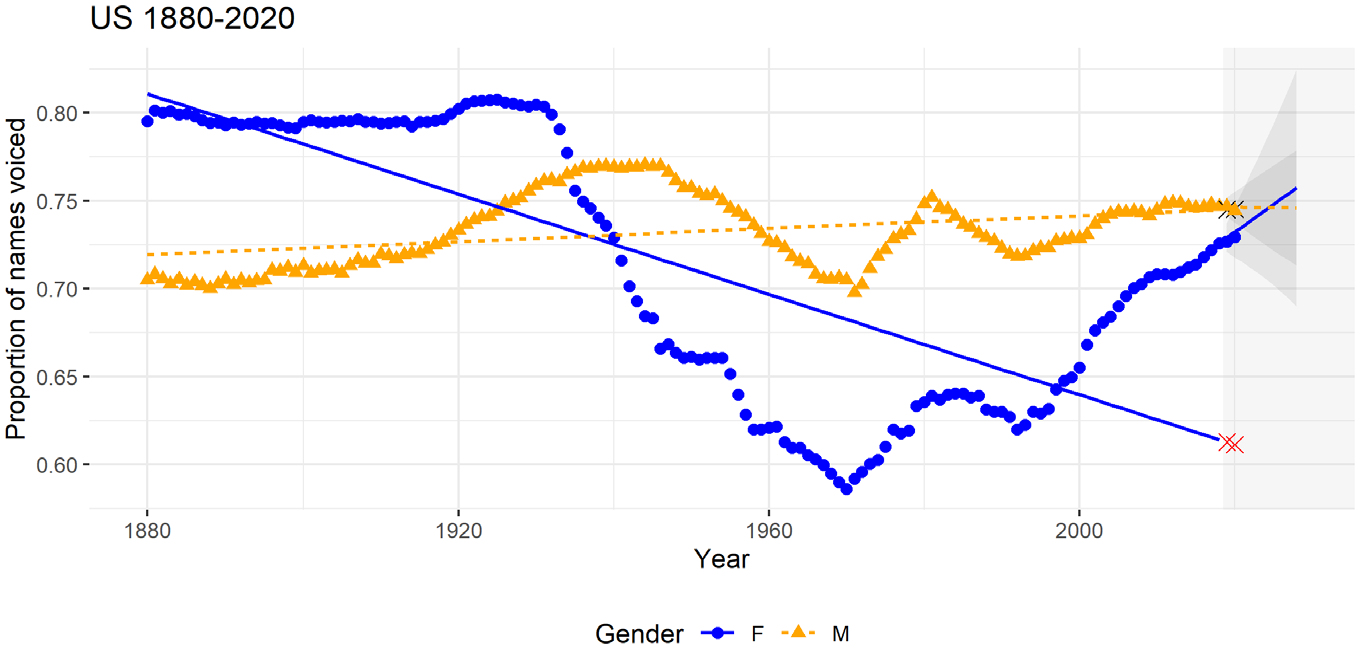
The Proportion of Female (Blue Dots) and Male Voiced Names (Orange Triangles) Given to Newborns in the United States Between 1880 and 2020, With Multilevel Regression Lines for 1880–2018 From Vishkin et al. (2022)

A method that provides predictions for future year while taking dependence between timepoints into account is time series analysis (see e.g. Wei, 2013). Time series may include a drift-term if there is evidence of a systematic change over time—such as if the proportion of voiced names significantly increases over time for male names and decreases for female names, respectively. I therefore used the “auto.arima” function in the “forecast” R-package to extract the best-fitting time series model for the boys’ and girls’ proportions in the U.S. data over the years 1880–2018 (the English and Welsh data have too few timepoints) and predicted 10 years into the future.

The resulting predictions consist of a best prediction line and an interval in which 95% of trajectories are expected to be included. As illustrated in Figure 2, these models predict more appropriately. The fitted models did not include drift-terms, so there is no evidence of a systematic increased proportion of voiced names for boys nor a decreased proportion for girls, and thus, no increased differentiation. To examine the robustness of these results, I used the ‘Arima’ function in the same package to examine similar models as these but with a drift-term included. The drift-term was never even close to significance in these models (all ps > .350). I also examined time series for the difference in proportions (male minus female), which never showed any systematic increased differentiation either (all drift-term ps > .150). See Supplemental Section 1.4 for details.

Thus, plotting the data and using methods that account for dependence between years have shown that there is no support for the conclusion that the proportions have differentiated nor that they will continue to differentiate over time. This fits well with what, to the best of my knowledge (surprisingly), appears to be the only study which has examined psychological gender differentiation as a function of gender equality over time ³ (Connolly et al., 2020), which, unlike the cross-cultural gender-equality paradox studies, did not find a paradox, and a decreased differentiation with time.

A Non-Representative Sample?

One final aspect of the U.S. dataset is interesting to consider: can we understand why the U.S. proportion of female voiced names dropped around 1940? Notably, the drop occurs around the Great Depression and the Second World War, turbulent times which, rather than gender equality, may have motivated more conservative values and stereotypes (Thórisdóttir & Jost, 2011).

Another important factor, however, may be reporting standards. As two of the authors of Vishkin et al. (2022) report in Slepian and Galinsky (2016):

many people born before 1937 did not apply for a social security card when it was then introduced. Thus, we a priori decided to use names from 1937 and on given that names prior to 1937 do a particularly poor job of creating a representative sample. (p. 513)

(These data consist of names of social security card holders.) In Slepian and Galinsky (2016), the authors examine the same “voiced” and “unvoiced” categorization of female and male names and use the same dataset (up to the years available), as in Vishkin et al. (2022), so the exclusion of names prior to 1937 is presumably because the authors believe those years do not provide a proper estimate of these proportions. This seems reasonable, as holders born in early years likely come from particular regions and economic backgrounds and are thus not a random subset of the population. In fact, the gradual drop in voiced female names also appears to coincide with a gradual expansion of the social security card to the full U.S. population. At its inception in 1937, its purpose was to register the working population, and even then, it excluded about 40% of workers. This system, for example, excluded domestic and agricultural workers, which included many African Americans. A decision to gradually expand its usage then came in 1943, but with an enumeration at birth system not starting until 1987. Thus, the exclusion in earlier years was not a random subset of the population, which likely affected the names being registered. See Supplemental Section 1.5 for details.

So, what happens to the results if we follow the procedure in Slepian and Galinsky (2016) and exclude years prior to 1937? Using the same method as the authors, ⁴ predicting the percentages, with year (mean-centered per multilevel model recommendations), gender (−0.5 for women, 0.5 for men), and their interaction as fixed effects and the intercepts for years (as a separate factor) as random factors, gives an overall intercept of 69.64 and the fixed-effect estimates as follows: gender, b = 8.35, t = 28.06, p < .001; year, b = 0.001, t = 0.06, p = .950; Gender × Year, b = −0.049, t = −3.93, p < .001 (illustrated in the Supplemental Section 1.5, Figure S3). Thus, by this model, men had voiced names more often, but over the years, the significant negative interaction means women’s proportion was predicted to increase more than men’s (or decrease less), so this model predicts a decreased differentiation, rather than the increase predicted by the authors’ model. Thus, even with the same problematic multilevel model, the conclusions depend on the inclusion of years prior to 1937. Acknowledging that even samples following 1937 may be biased and starting later, for example, in 1943, with the decision to expand the use of the social security card, would only make this predicted decreased differentiation even stronger—as can be noted by the pattern in Supplemental Figure S3 where the increased proportion of voiced names for girls in later years has been stronger than the change for boys and even stronger than predicted by this (still problematic) model. ⁵

Reevaluating Study 2

The authors use two measures of state-level gender equality, based on census data and provided by the journalists Hagan and Lu (2019)—“gender equality” and “female leadership” (original labels). Vishkin et al. (2022) considered female leadership the primary measure, for which they found a significant gender interaction. They did not find this interaction for gender equality, however, and did not discuss this discrepancy. Yet, to conclude that it is the gender equality in these measures that affects peoples’ gendered choices, it clearly would be a more robust result to find a significant interaction for both measures. When a significant association is only found for one measure, it is especially pertinent to consider whether some confounding factor particular to that measure may cause the association.

Is the Hypothesis Corroborated?

Figure 3 presents the proportion of voiced names and the gender difference in this proportion across states. As is already apparent by the authors’ own Figure S2 (p. 496), the proportion of voiced names tended to be higher for both genders in states toward the higher end of female leadership, although this difference was larger for boys. Thus, the fact that the proportions are higher for both genders does not appear to corroborate the hypothesis about parents’ preferences for optimal distinctiveness.

Figure 3

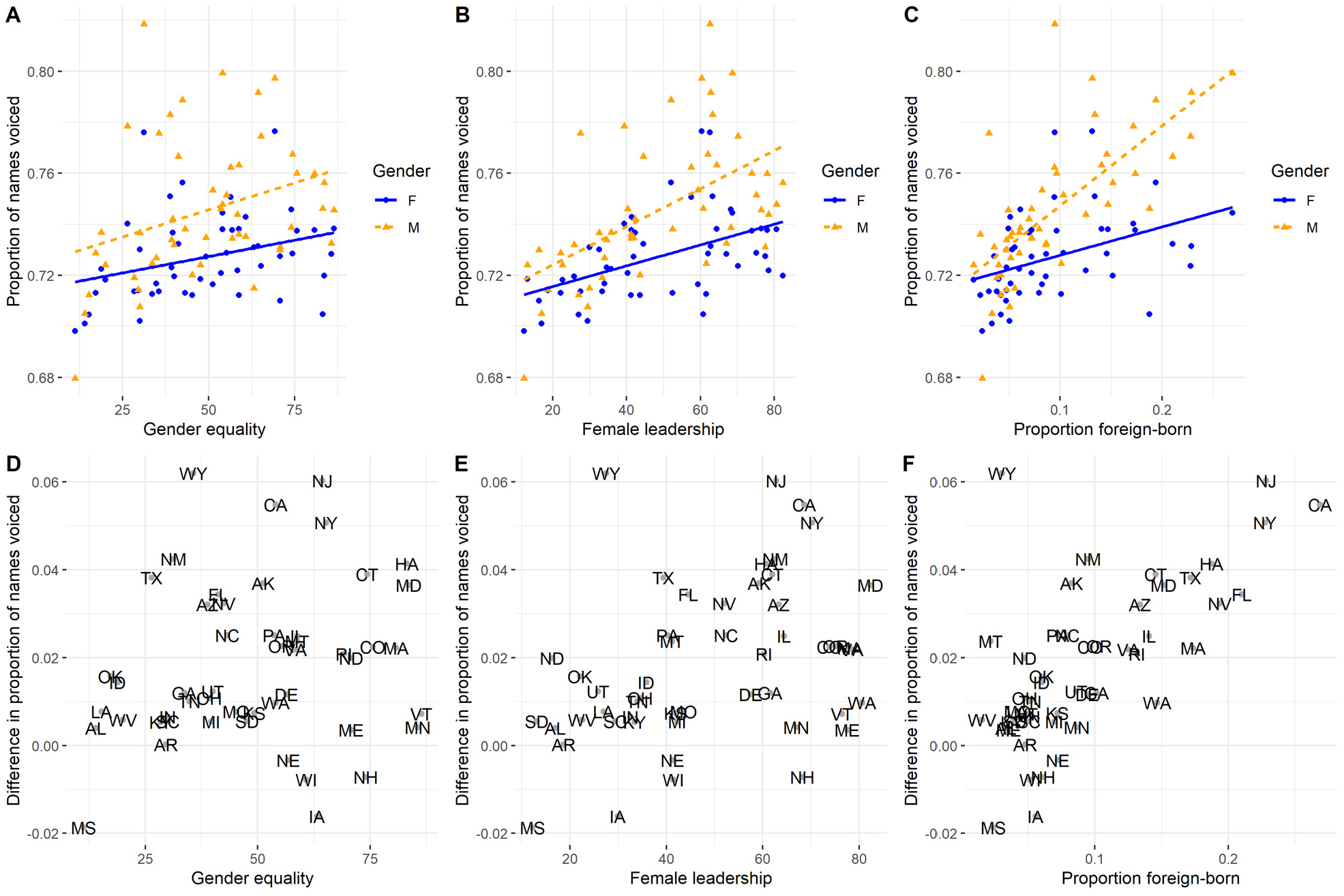
(A, B, and C) Proportion of Voiced Female and Male Names Given in the Year 2018 in the United States, With Simple Regression Lines. (D, E, and F) The Difference in Proportions (Male Minus Female), With State-Codes

The authors found a significant interaction and conducted simple slope analyses where they concluded that the increase for boys was significant, while the one for girls was not (p. 494). Thus, they considered their hypothesis corroborated. However, a reanalysis reveals issues with this conclusion. The authors present models with and without controls (see Table 1 in Vishkin et al., 2022, p. 495), but in all models, there is a significant main effect of 0.06 for female leadership and a significant interaction between female leadership and gender of 0.03–0.04 (depending on model). The authors present female leadership simple slopes of 0.01 for girls and 0.05 for boys.

Conversely, when I conducted simple slope analyses with the “sim_slopes” function in the “interactions” R-package, I found significant positive slopes of around 0.04 and 0.08 for girls and boys, respectively, no matter the model (ps < .05; see Supplemental Section 2.1 for details). So, what is going on? As only gender interacts with female leadership in all of the authors’ models, the simple slope estimates, barring roundoff-errors, should correspond to 0.06 + 0.03 × Gender ⁶ (or 0.06 + 0.04 × Gender depending on model), where Gender is coded −0.5 and 0.5 for female and male names, respectively. As male is coded 0.5 (>0), the simple slope for boys cannot be below 0.06, so the authors’ reported slope of 0.05 cannot possibly be correct if conducted as reported in the article. Similarly, the simple slope for girls should be around 0.06 + 0.03 × (−0.5) = 0.045 instead of the reported 0.01.

In summation then, recalculating the simple slopes of the models presented in the article revealed a significant increase in the proportion of voiced names in states with higher female leadership both for boys and girls. Thus, by what appears to be the authors’ predictions, these results do not provide much corroboration of the hypothesis of a differentiation due to a preference for optimal distinctiveness.

Controlling for Confounds

Even though the authors’ predictions do not appear corroborated, the significant interaction still suggests an increased difference. So, can this be ascribed to gender equality or is it merely due to confounding factors? One clear candidate confound is culture, which should have a strong influence on the names parents give to their children and which may therefore affect the relative proportions of voiced names. ⁷ The authors acknowledge this influence of culture/language, writing “baseline differences in the prevalence of different names between languages may vary greatly” (p. 494). Supporting that cultural differences may be influential, the three states in the upper half of female leadership with the largest gender differences, California, New Jersey, and New York, were also the top three U.S. states in the proportion of foreign-born inhabitants in 2018 (calculated from frequencies in Table B05012 from https://data.census.gov/cedsci/table, for 1-year interval, separated by states, retrieved April 27, 2022). Using these census data, I, therefore, examined how states’ proportions of voiced names varied with the proportion of foreign-born inhabitants. This is also illustrated in Figure 3, which shows that the proportion of foreign-born inhabitants predicts the differentiation in voiced names more strongly than does either gender equality or female leadership (a linear model predicting the proportion of voiced names with the proportion of foreign-born inhabitants, gender, and their interaction has an r² of .49; while corresponding models with gender equality or female leadership have r² = .23 and r² = .39 respectively). The increase in the male proportion of voiced names is especially notable. In line with the idea that the significant relationship for female leadership may be due to confounding factors, the proportion of foreign-born inhabitants had a stronger correlation with female leadership, r(48) = .57, p < .001, than with gender equality, r(48) = .35, p = .012. Furthermore, the association between female leadership and the gender differentiation disappeared when controlling for the proportion of foreign-born inhabitants and its gender interaction: adding the interaction between female leadership and gender had a non-significant effect, χ²(1) = 0.03, p = .857. This lack of association with controls was stable to variations in how controls were conducted. See Supplemental Section 2.2 for details. Thus, there was no state-association between female leadership and gender differentiation that could not be better explained by states’ proportion of foreign-born inhabitants.

Conclusion

In summation, the authors’ conclusions stem from problematic statistical methods and calculations. Using more appropriate methods, I found no support for their hypothesis nor for the idea that gender equality causes larger gender differences. In Study 1, the only sustained period of decrease for the female proportion occurs due to the inclusion of a time period two of the authors previously deemed to “do a particularly poor job of creating a representative sample” (Slepian & Galinsky, 2016, p. 513). In later years, the female proportion has instead been increasing, contrary to the direction predicted by the authors’ hypothesis. Furthermore, time series analysis, which accounts for the dependence between years, shows no overall trend for the male proportion to increase nor for the female proportion to decrease (nor for there to be an increased difference). In Study 2, recalculating the simple slopes showed that the male and female proportions, contrary to the hypothesis about a preference for optimal distinctiveness, are both higher in states with higher female leadership. Plotting the data further shows a decreased difference with time, as can be expected if voiced names are treated more gender-neutrally. This corroborates the only examination of gender differentiation and gender equality over time, which did not find a gender-equality paradox (Connolly et al., 2020), and thus similarly challenges the causal interpretation of this paradox (p. 111). Furthermore, there was no increased difference in states with higher female leadership that was not better explained by states’ proportion of foreign-born inhabitants.

In addition to highlighting the importance of appropriate statistical methods, this reexamination thus also illustrates the often-repeated problem of drawing causal conclusions from correlational observational data—where a multitude of confounding factors may influence the results. In Study 2, the association between gender equality and gender differentiation is confounded with a stronger cultural predictor of the latter—the proportion of foreign-born inhabitants. Previous studies on the gender-equality paradox have primarily assessed differences across countries (e.g., Falk & Hermle, 2018; Mac Giolla & Kajonius, 2019; Schmitt et al., 2008; Stoet & Geary, 2018; Vishkin, 2022), where cultural factors may be highly influential. Thus, when the gender-equality paradox was here only found with increasing cultural confounds (female leadership was more strongly associated with the proportion of foreign-born inhabitants than was gender equality), this may be in line with why other such paradoxes have been found cross-culturally (see, e.g., Berggren & Bergh, manuscript in preparation; Breda et al., 2020; Guimond et al., 2007; Vishkin, 2022; Wood & Eagly, 2012).

The re-examination of Study 1 revealed another likely important confounding factor—the subset of the population being registered. Other than earlier years unequally excluding African Americans, the early U.S. data are biased toward the working population specifically, and then only particular subsets of that working population. As the uses of the social security card broadened, it likely also specifically picked up people who had these uses for the card, and the further back you go in the data, the larger the proportion of the population who never lived long enough to have reason to register for it. As illustrated by the residuals from the time series analysis in Figure S2 in the Supplemental Section 1.4, the female proportion in particular shows a change in behavior in earlier years compared to in later ones, which may be a further indicator of a biased registering in earlier years. In addition, there are other possible confounds over time. As previously noted, the drop for girls (if some is real) occurs in connection to a turbulent time period, which, rather than gender equality, may have driven these changes (Thórisdóttir & Jost, 2011). In addition, the results of the cultural controls in Study 2 open up another possibility—if the cultural composition of the United States has become more heterogeneous with time, then the changes over time maybe driven by the inclusion of new name-traditions. This illustrates that also over time, there are many confounding factors that may make it difficult to parse out effects of gender equality. Whatever the ultimate cause of the variations though, the data do not support an overall trend for voiced male names to increase, voiced female names to decrease, nor the difference to increase, as predicted by a gender-equality paradoxical account.

Finally, these results may provide some suggestions on statistical best practices. First, as shown in the simulations, dependence dramatically increases error rates using the method in Vishkin et al. (2022) Study 1 (this also applies to ordinary linear regression). If multiple independent subjects are observed over time, multilevel models grouped by subjects with random slopes for the time-effects may control for this (see Section 1.2 in Bates et al., 2015). If the data cannot be grouped by independent subjects, then time series analysis as employed here is an alternative (see Wei, 2013). Dependence between subjects (whether because of time or other factors) should thus always be considered.

Another simple suggestion is to plot and examine basic properties of the data whenever possible. Had the proportions per year been plotted as is (rather than solely being represented through the models in Vishkin et al., 2022, Figure S1), then reviewers might have observed the need for the authors to clarify their statistical hypothesis and discuss alternative explanations for the resulting convergence.

Supplemental Material

sj-pdf-1-spp-10.1177_19485506221134353 – Supplemental material for No Evidence of a Gender-Equality Paradox in Gendered Names: Comment on Vishkin, Slepian, and Galinsky (2022)

Supplemental material, sj-pdf-1-spp-10.1177_19485506221134353 for No Evidence of a Gender-Equality Paradox in Gendered Names: Comment on Vishkin, Slepian, and Galinsky (2022) by Mathias Berggren in Social Psychological and Personality Science