Sage Journals: Discover world-class research

Abstract

Objective

The purpose of this work was to compare measurements of talar cartilage thickness and cartilage and bone surface geometry from clinically feasible magnetic resonance imaging (MRI) against high-accuracy laser scan models. Measurement of talar bone and cartilage geometry from MRI would provide useful information for evaluating cartilage changes, selecting osteochondral graft sources or creating patient-specific joint models.

Design

Three-dimensional (3D) bone and cartilage models of 7 cadaver tali were created using (1) manual segmentation of high-resolution volumetric sequence 3T MR images and (2) laser scans. Talar cartilage thickness was compared between the laser scan– and MRI-based models for the dorsal, medial, and lateral surfaces. The laser scan– and MRI-based cartilage and bone surface models were compared using model-to-model distance.

Results

Average cartilage thickness within the dorsal, medial, and lateral surfaces were 0.89 to 1.05 mm measured with laser scanning, and 1.10 to 1.22 mm measured with MRI. MRI-based thickness was 0.16 to 0.32 mm higher on average in each region. The average absolute surface-to-surface differences between laser scan– and MRI-based bone and cartilage models ranged from 0.16 to 0.22 mm for bone (MRI bone models smaller than laser scan models) and 0.35 to 0.38 mm for cartilage (MRI bone models larger than laser scan models).

Conclusions

This study demonstrated that cartilage and bone 3D modeling and measurement of average cartilage thickness on the dorsal, medial, and lateral talar surfaces using MRI were feasible and provided similar model geometry and thickness values to ground-truth laser scan–based measurements.

Keywords

cartilage talus MRI 3D model laser scan

Introduction

The ability to accurately measure talar cartilage thickness and create talar cartilage and bone surface models from clinical magnetic resonance imaging (MRI) has many potential applications, including preoperative planning of osteochondral defect treatment,^1-3 evaluation of osteoarthritis progression and treatment response^4,5 and research applications such as subject-specific biomechanical modeling.^6-9

Ankle MRI allows noninvasive evaluation of macroscopic and ultrastructure composition/organization cartilage changes.^10,11 Quantitative MRI such as T2,^10-13 T2*,¹⁴ T1rho,¹⁵ dGEMRIC,^11,16 sodium,¹⁷ and gagCEST¹⁸ mapping provide compositional information about cartilage tissue health and repair tissue quality,^17,19,20 while morphological sequences provide information about macroscopic characteristics such as synovitis, chondral/osteochondral lesions, subchondral bone cysts, and bone marrow edema.^10,11,21

MRI also has the capability of providing bone and cartilage 3-dimensional (3D) models and measurements. Measurement of cartilage thickness and thickness change provides information about cartilage health and is related to osteoarthritis progression and severity.^4,5 Image-based modeling of 3D talus morphology has been used for implant design²² and preoperative planning,^1-3,22 and creation of patient-specific biomechanical models.^6-9,23,24 In contrast to computed tomography, the standard clinical imaging modality for creation of bone models, MRI allows modeling of both bone and cartilage. Cartilage geometry models and thickness measurements provide additional information for joint contact modeling and implant design/selection.

Talar dome cartilage thickness has been measured invasively in cadaveric specimens using techniques such as needle-probe measurement,²⁵ stereophotagraphy,²⁶ and direct or radiographic measurement on talus cross-section cuts.^6,27 Noninvasive measurement methods have included operator-specific 2D methods such as ultrasound imaging, which has been used in living human subjects.^28,29 In contrast to ultrasound measurements, high-resolution MRI is capable of 3D thickness modeling over the entirety of the cartilage surfaces of interest, and allows modeling of both overlying soft tissue and underlying talar bone. High-resolution MRI has been shown to be capable of creating high accuracy cartilage models in joints such as the knee,³⁰ and has been used to examine ankle tibial plafond and talar dome cartilage geometry^4,31,32 and cartilage strains under physiological loading.^6-8 In the ankle, morphological imaging challenges are increased relative to other joints due to thin, curved, and highly congruent cartilage surfaces,¹⁰ making validation of MRI-based cartilage models against ground-truth models important. However, MRI-based cartilage thickness accuracy relative to a ground-truth 3D model has not yet been evaluated in the medial and lateral talar regions, and the accuracy of talus cartilage surface and bone 3D surface models from MRI have not been evaluated.

The purpose of this work was to compare measurements of talar cartilage thickness and cartilage and bone surface geometry from clinically feasible MRI against high-accuracy laser scan models. This study focuses on the ability of MRI to determine cartilage thickness and cartilage and bone geometry of the medial, lateral, and dorsal cartilage surfaces. Accurate MRI-based thickness modeling of the talar cartilage could have an impact on surgical decision making when selecting osteochondral grafts in patients with osteochondral lesions. Additionally, obtaining cartilage thickness and cartilage and bone surface geometry from MRI may assist in measurement of cartilage and bone changes and degradation in conditions such as osteoarthritis, and has applications in further research on the ankle joint.

Methods

Image Acquisition

This study used 7 nonpaired fresh-frozen ankle specimens (tibial plateau to toe-tip, 2 female and 5 male donors, mean age 44 ± 15 years, range 24-64 years). Donors with known osteoarthritis, osteoporosis, bone metastases, degenerative joint disease, sepsis, ankle surgery, or body mass index outside the age range of 18 to 35 years were excluded. Approximately 15 cm³ of ultrasound gel were injected using an anteromedial approach into each ankle joint prior to MRI scanning to simulate synovial fluid, slightly distend the joint, and minimize susceptibility artifact due to air³³ within the joint. MR imaging was performed with each specimen placed supine and positioned within a 16-channel receive-only clinical foot/ankle coil (Siemens Healthineers, Erlangen, Germany). Images were acquired on a Siemens MAGNETOM SkyraFit 3T scanner (Siemens Healthineers, Erlangen, Germany) using a gradient-echo T1-weighted volume interpolated breath-hold exam (VIBE) sequence in the sagittal plane. The images were acquired with the sequence parameters listed in Table 1 . The field of view was set to capture the entire ankle and hindfoot (approximately 14 cm in each direction) with the talus approximately centered in the field of view.

Table 1.

Magnetic Resonance Imaging Sequence Parameters for (Volume Interpolated Breath-Hold Exam) VIBE Sequence.

Plane	Sagittal
Number of slices	160
Slice thickness, mm	0.50
Field of view, mm × mm	125 × 125
Slice resolution, mm × mm	0.24 × 0.24
Acquisition matrix	256 × 256
Interpolated image matrix	512 × 512
Echo time, ms	5.60
Repetition time, ms	11.20
Flip angle, deg	10
Sequence variant	Spoiled, oversampling phase
Fat suppression	On—water excitation
Number of averages	1
Acquisition time, minutes:seconds	6:00

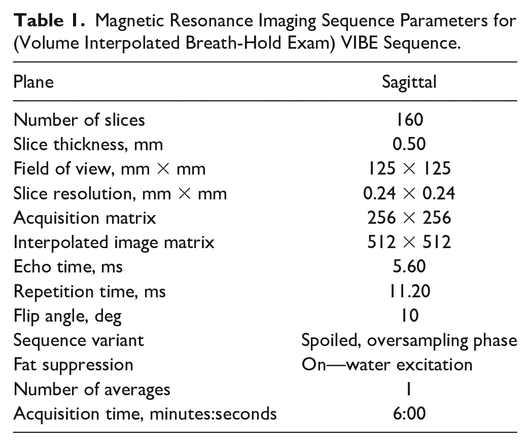
Image Analysis

The reconstructed sagittal plane MR images for each specimen were imported into 3D Slicer (http://www.slicer.org), an open source software platform for medical image processing and 3D visualization.³⁴ Fig. 1a-c illustrates the appearance of the sagittal segmentation images ( Fig. 1a ), and the coronal ( Fig. 1c ) and axial images ( Fig. 1b ) reconstructed from the sagittal image data that were displayed alongside the sagittal segmentation images for reference to improve visualization of the medial and lateral portions of the cartilage where partial volume averaging in the sagittal plane views makes visualization more challenging. The talus bone and talar dome cartilage were segmented by 2 raters (MD and IS) in the sagittal plane using thresholding and manual editing on a slice-by-slice basis using a touchscreen and stylus. Fig. 1d shows an example manual segmentation mask for bone and cartilage on one sagittal MR image slice.

Figure 1.

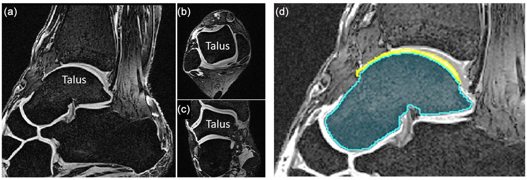
Magnetic resonance images of example ankle specimen with talus labeled, as viewed in the sagittal (acquisition) plane (a), axial reconstruction plane (b), and coronal reconstruction plane (c), and example bone (cyan) and cartilage (yellow) segmentation masks (d).

Laser Scanning

After MRI, the talus was dissected from the ankle joint and the remaining soft tissue was carefully mechanically removed using a No. 15 blade scalpel and curette with care taking to ensure no damage to the articular cartilage. The cartilage was kept moist with saline soaked gauze to avoid loss of thickness due to dehydration. Five fiducial markers were drilled using a surgical pin in areas free of cartilage on the lateral neck, superior neck, medial neck, medial body, and posterior body of the talus. These fiducial points were recorded into the digital coordinate frame using a ROMER Absolute Arm (Hexagon Metrology Inc., Oceanside, CA). Anterior-posterior lines on each talar shoulder defining the borders between the dorsal surface and the medial and lateral surfaces were also recorded with the ROMER arm for each specimen.

Each specimen was spray-coated with a thin, even layer of gray, matte chalk-paint (Rust-oleum Corporation, Vernon Hills, IL, USA) to reduce surface reflectivity artifact during laser scanning. Laser scans of each specimen were obtained using a HP-L-8.9 (Hexagon Manufacturing Intelligence, North Kingstown, RI, USA) laser scanner head mounted on a ROMER arm. The resulting point clouds were converted to STL models in GeoMagic Wrap (3D Systems, Inc., Rock Hill, SC, USA). The laser scan used acquires data points at 0.08 mm intervals with 0.04 mm accuracy.³⁵

After obtaining laser scans of all specimens with intact cartilage the specimens were soaked in bleach (sodium hypochlorite 1%-5%, Top Job Bleach, KIK Custom Products, Inc., Concord, Ontario, Canada) at room temperature for 72 hours, changing the bleach every 24 hours, until the cartilage was fully dissolved, and only bone remained. Bone-only talus models were then created using the laser scan steps described previously, with fiducial markers recorded again to put the bone-only models into the same coordinate frame as the previous bone-with-cartilage models.

Three-Dimensional Modeling

Laser scan-based 3D models were calculated from the laser scan point cloud data and exported, with both bone-only and bone-with-cartilage models in the same coordinate frame. MRI-based 3D models for each specimen were created from the manual segmentation masks in 3D Slicer using a marching cubes algorithm³⁶ and subsequently smoothed with a windowed-sinc filter (50 iterations) to reduce stair-step appearance resulting from the slice thickness.³⁷ For each specimen, the corresponding laser scan-based model file was imported into 3D Slicer. The MRI-based bone models were rigidly registered to the laser scan-based bone models using an iterative closest point algorithm³⁸ and the registration transformation matrix was then applied to the MRI-based cartilage model to align it with the other models. The MRI-based cartilage thickness was calculated using signed closest point distances³⁹ between the articular surface of the cartilage and the superficial surface of the subchondral bone at each vertex of the cartilage model for comparison with the laser scan-based cartilage thickness results. This closest point distance equaled the shortest straight-line distance between each vertex on the subchondral bone surface and the nearest corresponding vertex on the articular cartilage surface. This calculation results in a cartilage thickness measurement in millimeters at each vertex on the cartilage model articular surface. A similar approach was used to calculate the MRI-based model to laser scan model signed closest point distances for the cartilage and bone surface models. The 3D models and the lists of closest point distances at each model vertex were exported.

A custom MATLAB script was used to extract the thickness and model-to-model difference closest point distances for model vertices within each of the 3 regions of interest for each specimen. The average cartilage thickness on the medial, lateral, and dorsal talar surfaces was calculated for each MRI- and laser scan-based model, and the average absolute and root mean square (RMS) MRI-to-laser scan model differences were calculated within the script. The script imported the 3D models, closest point distances assigned to each model surface vertex, and the medial and lateral dorsal surface boundary points defined previously with the ROMER arm. Additional border points were manually selected by the MATLAB script operator to define the anterior and posterior borders of the talar dome cartilage, and the anterior/inferior/posterior borders of the medial and lateral cartilage regions. The manually selected points were defined on the first round of MRI cartilage models and saved, so that the same specimen-specific region border points were used on all models (MRI and laser, bone and cartilage) for each specimen. This allowed the exact same region borders to be used for all measurements on each specimen across the various models. The script extracted the cartilage thickness values for each of the 3 regions and calculated cartilage thickness summary statistics.

Additionally, in 3D Slicer 19 nonoverlapping circular cartilage thickness measurement subregions with a diameter of 0.5 cm were defined over the cartilage surface (5 medial, 5 lateral, and 9 dorsal subregions) to provide comparison measurements for correlation analysis over the range of talar dome cartilage thickness. The subregion locations are shown in Fig. 2. The subregions were defined on each laser scan-based model, then projected onto the registered MRI-based model (from a single MRI segmentation round for one rater). Mean cartilage thickness within each of these regions was calculated for the MRI- and laser scan-based models for all specimens and used for a correlation analysis.

Figure 2.

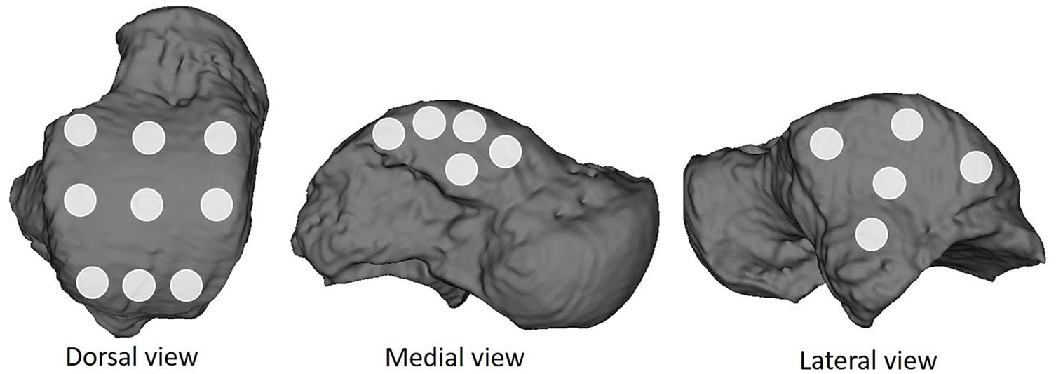
Nineteen circular subregions used for correlation analysis visualized on one example talus magnetic resonance imaging model.

In addition, surface-to-surface distances between the MRI- and laser scan–based cartilage and bone surface models within the medial, lateral, and dorsal regions were extracted. The average MRI- and laser scan–based cartilage thicknesses and average cartilage and bone model absolute surface-to-surface distances were compared for each region.

Statistical Analysis

Statistical analysis was performed using the statistical package R (R Development Core Team, Vienna, Austria⁴⁰). A paired t test was used to test for significant differences between the mean MRI thickness averaged over the rater rounds and the laser scan thickness for the 3 regions. The rater reliability for cartilage thickness, as generalizable to a single future rater, was evaluated over all specimens for the medial, lateral, and dorsal regions between 2 single rounds for 1 rater (intrarater) and between 2 different raters (interrater) using the intraclass correlation coefficient (ICC) for a 2-way random effects model of absolute agreement. The Pearson correlation test was used to look for correlations between the MRI- and laser scan–based mean cartilage thickness measurements for the 19 circular subregions for all regions combined and for the medial, lateral, and dorsal surface subregion groups.

Results

Seven nonpaired fresh-frozen ankle specimens (tibial plateau to toe-tip) less than the age of 65 years were used for this study. Specific donor age and sex for each specimen were unavailable.

Cartilage and Bone Comparison Results

The results for the average laser scan– and MRI-based cartilage thicknesses for each of the 3 talar cartilage regions are listed in Table 2, with an example for 1 specimen visualized in Fig. 3. The average absolute difference in thickness for the 3 regions between the average of the 3 MRI rater rounds and the laser scan-based models ranged from 0.16 to 0.32 mm. The difference in mean thickness for the talar dome between the MRI and laser measurements (laser scan mean thickness 0.32 mm less than MRI mean thickness) was found to be statistically significant (P = 0.003). No significant differences were found for the medial or lateral zones (mean cartilage thickness difference of 0.21 mm and P = 0.088 for the medial zone and 0.16 mm and P = 0.060 for the lateral zone).

Table 2.

Laser and Magnetic Resonance Imaging (MRI)–Based Cartilage Thickness for All Regions Averaged over All Specimens.

	Mean Thickness ± Standard Deviation (mm)		MRI Minus Laser Difference in Mean Thickness ± Standard Deviation(95% Confidence Interval) (mm)
Region	Laser Model	MRI Model(Average of 3 Rounds)
Dorsal surface	0.90 ± 0.21	1.22 ± 0.11	0.32 ± 0.16* (0.16-0.48)
Medial surface	0.89 ± 0.22	1.10 ± 0.09	0.21 ± 0.25 (−0.04 to 0.45)
Lateral surface	1.05 ± 0.21	1.21 ± 0.11	0.16 ± 0.17 (−0.01 to 0.34)

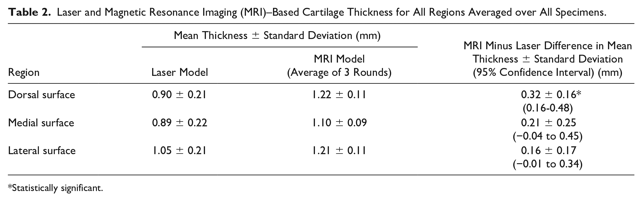
Statistically significant.

Figure 3.

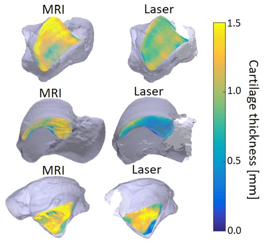
Local thickness plots for one specimen from both the magnetic resonance imaging (MRI)–based model (left) and the laser scan–based model (right) for the talar dome surface (top), the medial surface (middle), and the lateral surface (bottom).

The results of the 19-subregion cartilage thickness correlation analysis showed a significant “weak”⁴¹ positive correlation between MRI- and laser scan–based measurements for all subregions combined (ρ = 0.32, P < 0.001) and for the lateral subregion group (ρ = 0.35, P = 0.042), and a significant “moderate”⁴¹ positive correlation for the dorsal subregions (ρ = 0.46, P < 0.001). For the medial surface subregions the MRI and laser scan measurements did not show a significant correlation (ρ = 0.08, P = 0.640).

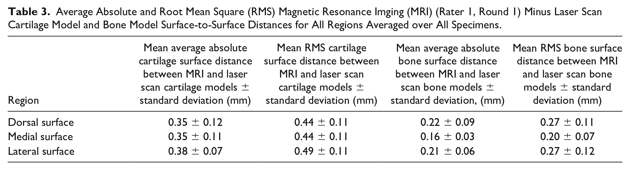
The average absolute surface-to-surface distances for the laser scan– versus MRI-based cartilage models are listed in Table 3 , with an example for one specimen visualized in Fig. 4 (cartilage differences) and Fig. 5 (bone differences). On average, the MRI-based bone surfaces were smaller than the laser scan–based bone surfaces, while the MRI-based cartilage surfaces were larger on average than the laser scan–based cartilage surfaces.

Table 3.

Average Absolute and Root Mean Square (RMS) Magnetic Resonance Imging (MRI) (Rater 1, Round 1) Minus Laser Scan Cartilage Model and Bone Model Surface-to-Surface Distances for All Regions Averaged over All Specimens.

Region	Mean average absolute cartilage surface distance between MRI and laser scan cartilage models ± standard deviation (mm)	Mean RMS cartilage surface distance between MRI and laser scan cartilage models ± standard deviation (mm)	Mean average absolute bone surface distance between MRI and laser scan bone models ± standard deviation, (mm)	Mean RMS bone surface distance between MRI and laser scan bone models ± standard deviation (mm)
Dorsal surface	0.35 ± 0.12	0.44 ± 0.11	0.22 ± 0.09	0.27 ± 0.11
Medial surface	0.35 ± 0.11	0.44 ± 0.11	0.16 ± 0.03	0.20 ± 0.07
Lateral surface	0.38 ± 0.07	0.49 ± 0.11	0.21 ± 0.06	0.27 ± 0.12

Figure 4.

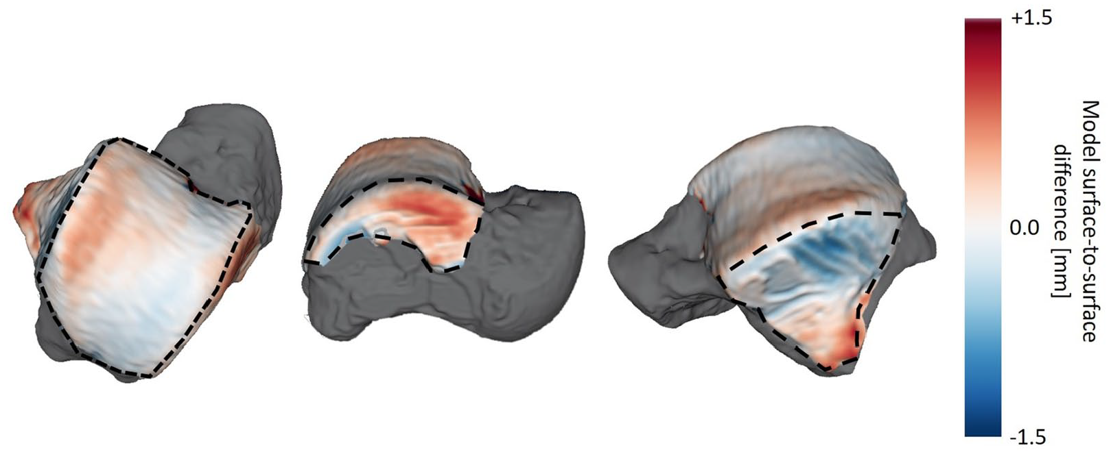
Local magnetic resonance imaging (MRI)–based cartilage model minus laser scan–based cartilage model surface-to-surface differences for one specimen. The surface-to-surface differences are color-mapped onto the MRI-based model with the surrounding bone surface shown in gray. The dorsal (left), medial (middle) and lateral (right) cartilage surfaces are outlined by black dashed lines.

Figure 5.

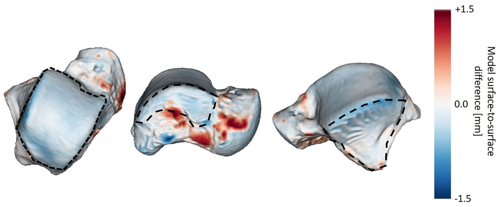
Local magnetic resonnce imaging (MRI)–based bone model minus laser scan–based bone model surface-to-surface differences for one specimen over the entire surface. The surface-to-surface differences are color-mapped onto the MRI-based model. The dorsal (left), medial (middle) and lateral (right) subchondral bone surfaces are outlined by black dashed lines.

Rater Reliability Results

Interrater absolute differences, calculated as the difference between the average cartilage thickness measured over 2 rounds by rater 1 and over a single round by rater 2 for the dorsal, medial, and lateral regions were 0.21 mm (range 0.02-0.61 mm across the 7 specimens), 0.18 mm (range 0.06-0.46 mm), and 0.20 mm (range 0.06-0.44 mm), respectively. Intrarater absolute differences in the average cartilage thickness over 2 rounds by rater 1 for the dorsal, medial, and lateral regions were 0.10 mm (range 0.01-0.44 mm across the 7 specimens), 0.10 mm (range 0.06-0.14 mm), and 0.10 mm (range 0.04-0.16 mm), respectively.

The ICCs for absolute agreement for each region were 0.35 (dorsal surface), 0.70 (medial surface), and 0.78 (lateral surface) for intrarater agreement and 0.10 (dorsal surface), 0.10 (medial surface), and 0.12 (lateral surface) for interrater agreement. The values for intrarater medial surface cartilage thickness was within the “fair to good” reliability category and lateral surface cartilage thickness was within the “excellent” category as designated by Fleiss⁴² (0.75-1.00 = excellent reliability, 0.40-0.75 = fair to good reliability, and 0.00-0.40 = poor reliability). The dorsal surface intrarater reliability and all interrater reliability values were within the “poor” range. Table 4 summarizes the agreement ICCs, 95% confidence intervals, bias, and limits of agreement.

Table 4.

Intra- and Interrater Agreement Intraclass Correlation Coefficient (ICC) Values for the Specimen Cartilage Thickness Values within the Dorsal, Medial, and Lateral Surfaces.

Region	Agreement ICC	Bias (mm_	95% Confidence Interval Lower Bound	95% Confidence Interval Upper Bound	Lower Limit of Agreement (mm)	Upper Limit of Agreement (mm)
Intrarater reliability
Dorsal surface	0.35	−0.07	−0.43	0.96	−0.41	0.27
Medial surface	0.70	0.04	0.41	0.82	−0.16	0.24
Lateral surface	0.78	−0.03	0.37	0.92	−0.26	0.20
Interrater reliability
Dorsal surface	0.10	−0.21	−0.27	0.61	−0.68	0.26
Medial surface	0.10	−0.16	−0.27	0.59	−0.48	0.17
Lateral surface	0.12	−0.19	−0.16	0.61	−0.53	0.14

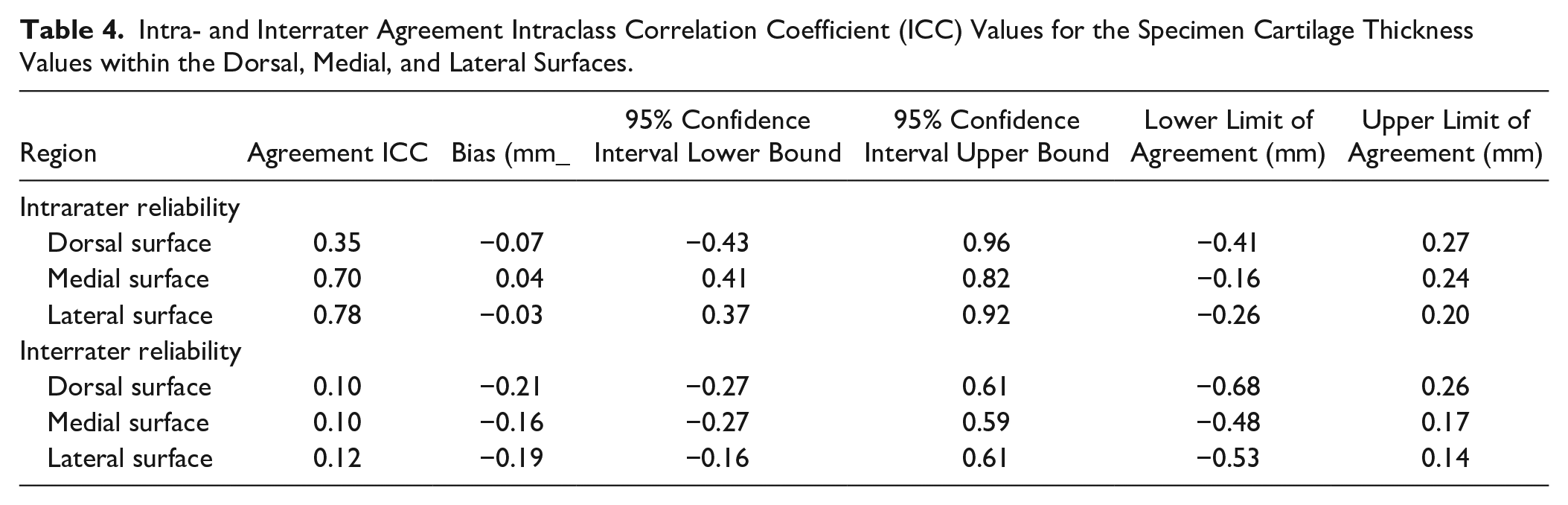
Fig. 6 shows the average cartilage thickness over all specimens for each region for laser scan–based measurements and measurements from MRI over 3 measurement rounds, illustrating average differences between the laser scan–based and MRI-based model thickness measurements and intra- and interrater differences.

Figure 6.

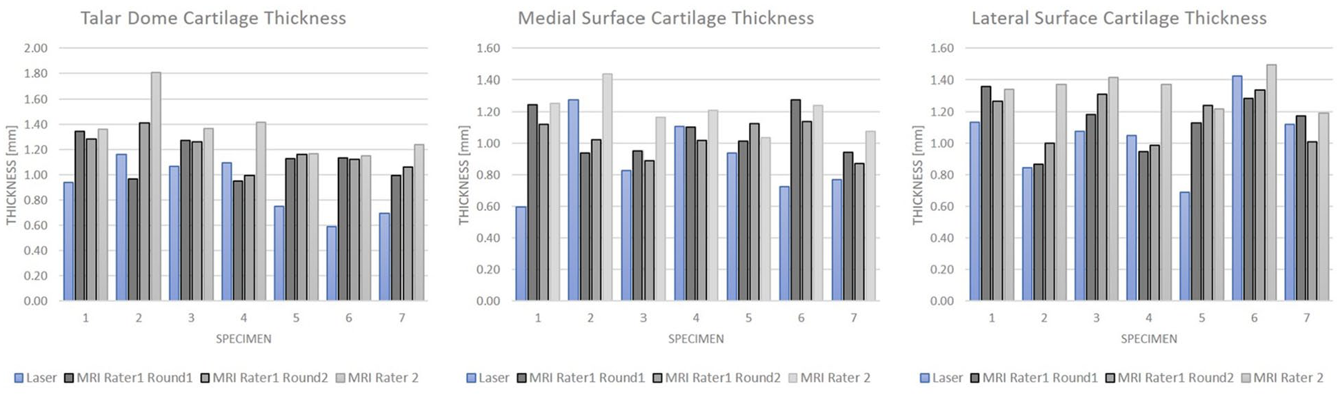
Graphs showing average cartilage thickness over all specimens for each region for laser scan-based measurements and measurements from magnetic resonance imaging over 3 measurement rounds.

Discussion

This study demonstrated that measurement of average cartilage thickness within the medial, lateral, and dorsal cartilage surface regions was comparable between MRI and laser scan-based measurements, with average absolute differences of 0.16 to 0.32 mm. Average MRI-based cartilage thickness was slightly higher than the thickness measured by laser scanning for all regions, demonstrating a tendency toward cartilage thickness overestimation when measured on MRI.

We found a mean dorsal surface cartilage thickness of 0.90 ± 0.21 mm with laser scanner and 1.22 ± 0.11 mm with MRI. Our mean MRI-based thickness is within the range of previously reported MRI-based measurements, which range from 0.89 ± 0.19 mm to 1.60 ± 0.10 mm.^4,6,24 Our laser scan–based dorsal cartilage mean thickness also falls within the range of reported measurements, between 0.82 and 1.62 mm, obtained using invasive measurement methods, such as contact 3D digitization,⁴³ needle displacement measurement,²⁵ stereophotagraphy,²⁶ and cross-section radiography²⁷ of cadaver specimens.

Our study is the first to directly compare the accuracy of MRI with ground truth laser scanning for assessment of talar cartilage thickness and cartilage and bone surface. Our results provide accuracy information for MRI-based measurements in future clinical and research settings that require noninvasive measurements. In the present study, the difference in cartilage thickness between MRI- and laser scan–based models was 0.16 ± 0.17 mm to 0.32 ± 0.16 mm over 3 analyzed talar cartilage regions. The thickness difference for the dorsal surface regions was statistically significant, while the medial and lateral zone differences were not found to be statistically significant. However, an a priori power analysis was not performed to determine the number of specimens required to detect a significant difference, so the comparison may be underpowered.

MRI- and laser scan–based thickness measurements extracted from 19 subregions over the talar dome cartilage surface were found to be significantly correlated. When grouped by zone significant correlations were found for the measurements within the lateral zone subregions and dorsal zone subregions, but not for the medial zone subregions. The correlation strength was strongest for the dorsal subregion (“moderate” correlation as defined by one stratification schemes used in the literature⁴¹) and “weak” for the combined subregions and for the lateral subregion alone. It is important to note that correlation strength is impacted by the range of values present,⁴¹ so the limited range of cartilage thickness values present on the talar dome surfaces may limit the correlation strength. The MRI-based thickness measurements on the medial surface were likely affected by the fact that the medial cartilage surface was oriented near-parallel to the MR image acquisition and segmentation plane. As such, small variations in cartilage thickness that were detected by the laser scanner become obscured by the MRI slice thickness. For applications where the medial cartilage thickness is important MR image acquisition should be performed in the coronal plane.

Direct surface-to-surface measurements between the MRI- and laser scan–based cartilage surface models showed similar results, with the MRI-based cartilage models being slightly larger than the laser scan–based cartilage models. This is in line with the results in a similar comparison performed in knee specimens, which predominantly demonstrated thicker cartilage models from MRI as compared to laser scan.⁴⁴ Average differences in thickness were 0.38 mm in regions where MRI underestimated cartilage thickness and 1.15 mm in regions where MRI overestimated cartilage thickness for tibial and femoral cartilage. An overall difference in average cartilage thickness of 0.09 ± 0.27 mm for femoral cartilage and 0.05 ± 0.19 mm for tibial cartilage has been reported.³⁰

Direct surface-to-surface comparison between the MRI- and laser scan–based subchondral bone surface models showed lower differences compared to the cartilage comparisons and showed that the MRI-based bone models were slightly smaller on average than the laser scan–based models with a mean absolute difference of 0.22 ± 0.09 mm at the dorsal, 0.16 ± 0.03 mm at the medial, and 0.21 ± 0.06 mm at the lateral talar surfaces. Although direct MRI- to laser scan–based bone model comparisons are rare in the literature, our results can be compared to previously reported results for other bones and for MRI versus computed tomography (CT) based bone models and laser scan– versus CT-based bone models. Our MRI versus laser scan bone model difference results were similar to work comparing proximal femur bone MRI-based models to laser scan-based models by Malloy et al.⁴⁵ They reported an average absolute surface-to-surface distance of 0.30 ± 0.08 mm over 6 cadaver proximal femur specimens for MRI versus laser scan-based models. In contrast to our results, their MRI-based bone models were slightly larger on average than those obtained with laser scanning. This may be due to differences in imaging protocol, such as larger voxels (0.9 mm isotropic) used by Malloy et al.⁴⁵ compared with our protocol. This lower resolution would increase the influence of partial volume averaging at the bone borders.

A greater number of reports in the literature have used CT as the gold standard for bone geometry modeling when evaluating the accuracy of MRI, although CT geometry has been shown to differ slightly from ground-truth results obtained by laser scanning (0.36 ± 0.13 mm average absolute difference for the proximal femur⁴⁵ and approximately 0.5 mm average absolute difference for the bones of the knee).⁴⁴ Our MRI versus laser scan results are in line with results for other bones for MRI versus CT and CT versus laser scan comparisons. Neubert et al.⁴⁶ reported that the MRI-based bone models were overall smaller than the CT-based bone models of the knee joint, although the difference was 0.61 mm or lower for the knee bones when comparing CT versus VIBE MRI models.

There are some limitations that must be considered. First, the use of cadaveric specimens results in greater ankle distraction in the neutral unloaded state during imaging than is generally present in living subjects, making separation of the talar and tibial articular surfaces more visible on the MR images, and eliminating the impact of motion and pulsatile flow artifacts on the MRI quality. Second, the injected ultrasound gel volume approached maximum ankle joint volume (20.9 ± 4.9 mL⁴⁷), contributing to exaggerated joint distention and articular cartilage surface separation observed in 3 specimens. Cadaver-specific segmentation difficulties are introduced by the lack of synovial fluid and magnetic susceptibility artifacts from ice damage and air infiltration. Joint space air bubbles near the articular surfaces did distort or obscure the talar cartilage in some locations, impacting segmentation reliability.

Another limitation of this work was poor cartilage thickness intra- and interrater reliability for the talar dome, and poor interrater reliability for all zones. The 2 raters measured cartilage thickness with average interrater differences of 0.20 mm when averaged over all regions and all specimens, with similar levels of difference across all regions. The average between-rater differences represent approximately 1 MRI pixel difference in cartilage thickness on average, illustrating how the limitations of MRI resolution can create a difference in thickness measurement that represents a large proportion of the total cartilage thickness for the very thin cartilage within the ankle joint. Al-Ali et al.⁴ reported coefficients of variation of 3.7% to 10.9% and stated that the precision between segmentation rounds for maximal thickness was in the range of 1-pixel width (0.125 mm in their study). Increased MRI resolution could improve precision in future applications of MRI-based joint modeling but must be balanced against decreased signal-to-noise levels and increased scan time. Development of automated segmentation methods may improve segmentation consistency and would improve the feasibility of MRI-based model creation for widespread use by reducing manual processing time requirements.

This study demonstrates the feasibility of measuring medial, lateral, and dorsal surface talar cartilage thickness on MRI and demonstrates the achievable accuracy of MRI measurements and 3D models of the cartilage and bone relative to a ground truth standard. Accurate MRI-based measurement of talar cartilage thickness and 3D cartilage and bone modeling may assist with preoperative planning, measurement of cartilage thickness changes with cartilage pathology, and patient-specific ankle joint modeling.

Footnotes

Author’s Note

This work was conducted at the Steadman Philippon Research Institute.

Acknowledgments and Funding

The author(s) received no financial support for the research, authorship, and/or publication of this article.

Declaration of Conflicting Interests

The author(s) declared no potential conflicts of interest with respect to the research, authorship, and/or publication of this article.

ORCID iDs

Carly A. Lockard

Kira K. Tanghe

References

Choi

Kim

Lee

JW.

Prognostic significance of the containment and location of osteochondral lesions of the talus: Independent adverse outcomes associated with uncontained lesions of the talar shoulder. Am J Sports Med. 2013;41(1_suppl):126-33. doi:10.1177/0363546512453302

Chuckpaiwong

Berkson

Theodore

GH.

Microfracture for osteochondral lesions of the ankle: Outcome analysis and outcome predictors of 105 cases. Arthroscopy. 2008;24(1_suppl): 106-12. doi:10.1016/j.arthro.2007.07.022

Ramponi

Yasui

Murawski

Ferkel

DiGiovanni

Kerkhoffs

GMMJ

, et al. Lesion size is a predictor of clinical outcomes after bone marrow stimulation for osteochondral lesions of the talus: a systematic review. Am J Sports Med. 2017;45(7):1698-705. doi:10.1177/0363546516668292

Al-Ali

Graichen

Faber

Englmeier

K-H

Reiser

Eckstein

Quantitative cartilage imaging of the human hind foot: precision and inter-subject variability. J Orthop Res. 2002;20(2):249-56. doi:10.1016/S0736-0266(01)00098-5

Iriondo

Liu

Calivà

Kamat

Majumdar

Pedoia

. Towards understanding mechanistic subgroups of osteoarthritis: 8-year cartilage thickness trajectory analysis. J Orthop Res. Published online September 8, 2020. doi:10.1002/jor.24849

Wan

de Asla

Rubash

In vivo cartilage contact deformation of human ankle joints under full body weight. J Orthop Res. 2008;26(8):1081-9. doi:10.1002/jor.20593

Bischof

Spritzer

Caputo

Easley

DeOrio

Nunely

2nd , et al. In vivo cartilage contact strains in patients with lateral ankle instability. J Biomech. 2010;43(13):2561-6. doi:10.1016/j.jbiomech.2010.05.013

Bae

Park

Seon

Jeon

Analysis of the effects of normal walking on ankle joint contact characteristics after acute inversion ankle sprain. Ann Biomed Eng. 2015; 43(12):3015-24 . doi:10.1007/s10439-015-1360-1

Wang

Roach

Kapron

Fiorentino

Saltzman

Singer

, et al. Accuracy and feasibility of high-speed dual fluoroscopy and model-based tracking to measure in vivo ankle arthrokinematics. Gait Posture. 2015;41(4):888-93. doi:10.1016/j.gaitpost.2015.03.008

10.

Schreiner

Mlynarik

Zbýň

Szomolanyi

Apprich

Windhager

, et al. New technology in imaging cartilage of the ankle. Cartilage. 2017;8(1_suppl):31-41. doi:10.1177/1947603516632848

11.

Van Bergen

Gerards

Opdam

Terra

Kerkhoffs

GM.

Diagnosing, planning and evaluating osteochondral ankle defects with imaging modalities. World J Orthop. 2015;6(11):944-53. doi:10.5312/wjo.v6.i11.944

12.

Lockard

Chang

Shin

Clanton

CP.

Regional variation of ankle and hindfoot cartilage T2 mapping values at 3 T: a feasibility study. Eur J Radiol. 2019;113:209-16. doi:10.1016/j.ejrad.2019.02.011

13.

Tao

Qiao

Yan

Hua

, et al. T2-mapping evaluation of early cartilage alteration of talus for chronic lateral ankle instability with isolated anterior talofibular ligament tear or combined with calcaneofibular ligament tear. J Magn Reason Imaging. 2018;47:69-77. doi:10.1002/jmri.25745

14.

Krause

Klammer

Benneker

Werlen

Mamisch

Weber

Biochemical T2* MR quantification of ankle arthrosis in pes cavovarus. J Orthop Res. 2010;28(12):1562-8. doi:10.1002/jor.21192

15.

Horiuchi

Luk

Rudd

Ton

Kuoy

, et al T1rho and T2 mapping of ankle cartilage of female and male ballet dancers. Acta Radiol. 2020;61(10):1365-76 . doi:10.1177/0284185120902381

16.

Rehnitz

Kuni

Wuennemann

Chloridis

Kirwadi

Burkholder

, et al. Delayed gadolinium-enhanced MRI of cartilage (dGEMRIC) and T2 mapping of talar osteochondral lesions: indicators of clinical outcomes. J Magn Reson Imaging. 2017;46(6):1601-10 . doi:10.1002/jmri.25731

17.

Zbýň

Stelzeneder

Welsch

Negrin

Juras

Mayerhoefer

, et al Evaluation of native hyaline cartilage and repair tissue after two cartilage repair surgery techniques with 23Na MR imaging at 7 T: initial experience. Osteoarthritis Cartilage. 2012;20(8):837-45. doi:10.1016/j.joca.2012.04.020

18.

Abrar

Schleich

Radke

Frenken

Stabinska

Ljimani

, et al. Detection of early cartilage degeneration in the tibiotalar joint using 3 T gagCEST imaging: a feasibility study. MAGMA. Published online July 28, 2020. doi:10.1007/s10334-020-00868-y

19.

Domayer

Apprich

Stelzeneder

Hirschfeld

Sokolowski

Kronnerwetter

, et al. Cartilage repair of the ankle: first results of T2 mapping at 7.0 T after microfracture and matrix associated autologous cartilage transplantation. Osteoarthritis Cartilage. 2012;20(8):829-36. doi:10.1016/j.joca.2012.04.015

20.

Domayer

Welsch

Stelzeneder

Hirschfeld

Quirbach

Nehrer

, et al. Microfracture in the ankle: clinical results and MRI with T2-mapping at 3.0 T after 1 to 8 years. Cartilage. 2011;2(1_suppl):73-80. doi:10.1177/1947603510380901

21.

Rosenberg

Beltran

Bencardino

JT.

MR imaging of the ankle and foot. Radiographics. 2000;20(Suppl 1):S153-S179. doi:10.1148/radiographics.20.suppl_1.g00oc26s153

22.

Islam

Dobbe

Duke

El-Rich

Dhillon

Adeeb

, et al. Three-dimensional geometric analysis of the talus for designing talar prosthetics. Proc Inst Mech Eng H. 2014;228(4):371-8. doi:10.1177/0954411914527741

23.

Anderson

Goldsworthy

Shivanna

Grosland

Pedersen

Thomas

, et al. Intra-articular contact stress distributions at the ankle throughout stance phase-patient-specific finite element analysis as a metric of degeneration propensity. Biomech Model Mechanobiol. 2006;5(2-3):82-9. doi:10.1007/s10237-006-0025-2

24.

Cher

Utturkar

Spritzer

Nunley

DeFrate

Collins

AT.

An analysis of changes in in vivo cartilage thickness of the healthy ankle following dynamic activity. J Biomech. 2016;49(13):3026-30. doi:10.1016/j.jbiomech.2016.05.030

25.

Shepherd

DET

Seedhom

BB.

Thickness of human articular cartilage in joints of the lower limb. Ann Rheum Dis. 1999; 58(1_suppl):27-34. doi:10.1136/ard.58.1.27

26.

Millington

Grabner

Wozelka

Anderson

Hurwitz

Crandall

. Quantification of ankle articular cartilage topography and thickness using a high resolution stereophotography system. Osteoarthritis Cartilage. 2007; 15(2):205-11. doi:10.1016/j.joca.2006.07.008

27.

Sugimoto

Takakura

Tohno

Kumai

Kawate

Kadono

Cartilage thickness of the talar dome. Arthroscopy. 2005;21(4):401-4. doi:10.1016/j.arthro.2004.12.005

28.

Song

Pietrosimone

Wikstrom

EA.

Comparison of talar cartilage thickness between those with and without chronic ankle instability: a ultrasonography study. Osteoarthritis Cartilage. 2019;27:S322-S323. doi:10.1016/j.joca.2019.02.724

29.

Yalçın

Kara

Öztürk

Özçakar

Ultrasonographic measurements of the metacarpal and talar cartilage thicknesses in hemiplegic patients after stroke. Top Stroke Rehabil. 2017;24(1_suppl):1-4. doi:10.1080/10749357.2016.1183357

30.

Thorhauer

Tashman

Validation of a method for combining biplanar radiography and magnetic resonance imaging to estimate knee cartilage contact. Med Eng Phys. 2015;37(10):937-47. doi:10.1016/j.medengphy.2015.07.002

31.

Tan

TCF

Wilcox

Frank

Shih

Trudell

Sartoris

, et al. MR imaging of articular cartilage in the ankle: comparison of available imaging sequences and methods of measurement in cadavers. Skeletal Radiol. 1996;25(8):749-55. doi:10.1007/s002560050173

32.

Trattnig

Breitenseher

Huber

Zettl

Rottmann

Haller

, et al. Determination of cartilage thickness in the ankle joint. an MRT (1.5)-anatomical comparative study [in German ]. Rofo. 1997;166(4):303-6. doi:10.1055/s-2007-1015429

33.

Farghadani

Rezei

Karami

Comparison of susceptibility artifact on rectal DWI-MRI and rectal volume before and after ultrasound gel versus Microlax enema. J Adv Pharm Edu Res. 2020;10(2):15-20.

34.

Fedorov

Beichel

Kalpathy-Cramer

Finet

Fillion-Robin

Pujol

, et al. 3D Slicer as an image computing platform for the quantitative imaging network. Magn Reson Imaging. 2012;30(9):1323-41. doi:10.1016/j.mri.2012.05.001

35.

Hexagon. Product brochure. Absolute arm. Accessed January 30, 2020. https://willrich.com/wp-content/uploads/2014/09/Hexagon-MI-Absolute-Arm-2018-Brochure-.pdf

36.

Lorensen

Cline

. Marching cubes: A high resolution 3D surface construction algorithm. In: Proceedings of the 14th Annual Conference on Computer Graphics and Interactive Techniques - SIGGRAPH ‘87. ACM Press; 1987:163-169. doi:10.1145/37401.37422

37.

Lehmann

Gonner

Spitzer

Survey: interpolation methods in medical image processing. IEEE Trans Med Imaging. 1999;18(11):1049-75 . doi:10.1109/42.816070

38.

Besl

McKay

ND.

A method for registration of 3-D shapes. IEEE Trans Pattern Anal Mach Intell. 1992;14(2):239-56. doi:10.1109/34.121791

39.

Quammen

Weigle

Taylor

Boolean operations on surfaces in VTK without external libraries. VTK J. 2011;797(1_suppl).

40.

R Core Team. R: a language and environment for statistical computing. Accessed January 27, 2020. http://www.R-project.org/

41.

Schober

Boer

Schwarte

LA.

Correlation coefficients: appropriate use and interpretation. Anesth Analg. 2018;126(5):1763-8. doi:10.1213/ANE.0000000000002864

42.

Fleiss

JL.

The Design and Analysis of Clinical Experiments. John Wiley & Sons, Inc; 1986.

43.

Akiyama

Sakai

Sugimoto

Yoshikawa

Sugamoto

Three-dimensional distribution of articular cartilage thickness in the elderly talus and calcaneus analyzing the subchondral bone plate density. Osteoarthritis Cartilage. 2012;20(4):296-304. doi:10.1016/j.joca.2011.12.014

44.

Thorhauer

Miyawaki

Illingworth

Holmes

Anderst

Accuracy of bone and cartilage models obtained from CT and MRI. Poster presented at: The 34th Annual Meeting of the American Society of Biomechanics; August 18-21, 2010; Providence, RI.

45.

Malloy

Gasienica

Dawe

Espinoza Orías

Nwachukwu

Inoue

, et al. 1.5 T magnetic resonance imaging generates accurate 3D proximal femoral models: Surgical planning implications for femoroacetabular impingement. J Orthop Res. 2020;38:2050-6. doi:10.1002/jor.24596

46.

Neubert

Wilson

Engstrom

Surowiec

Paproki

Johnson

, et al. Comparison of 3D bone models of the knee joint derived from CT and 3T MR imaging. Eur J Radiol. 2017;93:178-84. doi:10.1016/j.ejrad.2017.05.042

47.

Draeger

Singh

Parekh

SG.

Quantifying normal ankle joint volume: an anatomic study. Indian J Orthop. 2009; 43(1_suppl):72-5. doi:10.4103/0019-5413.45326

Accuracy of MRI-Based Talar Cartilage Thickness Measurement and Talus Bone and Cartilage Modeling: Comparison with Ground-Truth Laser Scan Measurements

Abstract

Objective

Design

Results

Conclusions

Keywords

Introduction

Methods

Image Acquisition

Image Analysis

Laser Scanning

Three-Dimensional Modeling

Statistical Analysis

Results

Cartilage and Bone Comparison Results

Rater Reliability Results

Discussion

Footnotes

Author’s Note

Acknowledgments and Funding

Declaration of Conflicting Interests

ORCID iDs

References