
Abstract
This research note draws attention to a novel choice-based conjoint (CBC) model by which guests’ preferences toward hotel room rate conditions can be predicted as a function of time. Through the model, the notion is explored whether willingness to pay for rate conditions (without penalty) depends on the size of the booking window. The modified choice model includes time as an additional “attribute.” This attribute does not present a feature of the choice propositions, but instead is associated with the choice context. An empirical study was carried out to demonstrate the proposed model using three common booking conditions (i.e., free cancelation, free date change, pay on departure). The results show significant and positive time-dependent mean components for cancelation and date change conditions. Despite a limited sample size, all significant effects have expected directions (no parameter reversals) providing evidence of the robustness of the model. The results indicate that the ability to cancel or change a booking is preferred more when the booking window is bigger. Accordingly, as the time period between the advanced purchase and intended date of arrival increases, the willingness to pay for rate conditions also increases. This finding has major practical implications for price and revenue optimization. Limitations of the proposed time-dependent model are discussed.
Introduction
The capacity constrained hotel industry has three strategic levers to maximize the revenue of rooms: the allocation of capacity, control of the length of stay, and optimization of the mix of prices and associated terms and booking conditions (Kimes & Renaghan, 2011). These levers enable hotels to reduce opportunity costs by stimulating demand from price-sensitive guests who are prepared to book early to help fill capacity. As rooms are service products that are produced and consumed simultaneously, any booking of rooms essentially is a form of advance selling (Ng & Lee, 2008). This time dimension of selling rooms implies that both hotels and guests face uncertainty. Hotels face a potential loss of revenue, whereas guests may be confronted with a higher priced or fully booked hotel (Ng, 2007). To reduce such uncertainty, some guests decide to book their room in advance (Shugan & Xie, 2004). Hotels employ forecasting, length of stay, and overbooking algorithms (Png, 1989), and set rate conditions such as the (in)ability to modify or cancel a booking in advance.
Setting rate conditions, such as on cancelation, is a widely used practice in hotel room rate pricing where several conditioned rates are generally offered in addition to an unconditioned rate. 1 A complicating factor for the application of rate conditions is that booking windows (i.e., the time interval between the date of the advanced booking and the day of arrival) vary over the booking horizon. That is, some guests book a room near the day of arrival, whereas others plan their trip way in advance (ceteris paribus). Although booking preferences may vary, in practice, hotels commonly keep the difference between (dynamically priced) conditioned and unconditioned room rates static over time. In other words, the surcharge that guests need to pay to book an unconditioned room rate (e.g., a room without cancelation penalty) is independent of the booking window.
Examining the differentiation of cancelation policies in the U.S. hotel industry, Chen and Xie (2013) confirm that “only static policies are observed across different search time points” (p. 70). They recommend investigations into a dynamic pricing approach to cancelation policies “in which the deadline and the price are changed based on the search time and the check-in dates” (Chen & Xie, 2013, p. 70). Hilton’s President and CEO Chris Nassetta recently announced the launch of such approach: “we’re taking it from 48 or 72 hours (cancellation windows) to seven days, and then seven days and beyond, with a flexible or semi-flexible pricing approach,” he said. “I think it’s going to . . . help us deal with this issue (of short-term cancellations) in a more meaningful way and a way that drives higher RevPAR growth” (Ricca, 2017). Confirming that the industry has just picked up on a dynamic pricing approach to cancellation policies, CFO Kevin Jacobs adds, “the company is ‘deep into the testing’ of this pricing module ‘and we like what we see’” (Ricca, 2017).
The aim of this article is, therefore, to draw attention to a novel time-dependent discrete choice model to predict consumer preferences and sensitivities for rate conditions at several booking windows, thereby answering to the call of Chen and Xie (2013). By modeling consumers’ choices toward rate conditions as a function of time, the notion is explored whether the preference for rate conditions, as well as willingness to pay (WTP), depends on the size of the booking window. This is of particular interest to hotel revenue maximization in practice as Chen, Schwartz, and Vargas (2011) and Smith, Parsa, Bujisic, and Van der Rest (2015) have found that the amount of the cancelation fee does not change a guest’s booking decision. Indeed, the lodging industry collected an estimated US$2.9 billion in cancelation fees in 2018 (Elliott, 2019). Yet, as online travel agencies (OTAs), which generate the bulk of online distribution, push free cancelation policies, resulting in the cancelation of almost 40% of the on-the-books revenue in 2018 (Hertzfeld, 2019), with more and more travel programs allowing corporate travelers to book nonnegotiated hotel rates, determining the right advanced purchase rates at varying booking windows next to the best available rate (BAR) may thus become of increasing importance, especially if one considers the effects of high cancelations rates such as not being able to resell the room at the original rate, rate dropping, and challenges for the smooth functioning of forecasting, pricing, and overbooking algorithms (McCune, 2017).
Theoretical Perspective
To predict preferences for rate conditions as a function of time, we draw on the theory of discounted utility. Advances in this area, in economics, psychology, and more recently in neuroscience, reveal a complex account of intertemporal choice resulting from the splicing of two neural systems, each with different perspectives toward the future (Berns, Laibson, & Loewenstein, 2007). These intertwined systems predict how consumers make trade-offs between delaying an outcome (which can increase its size) and obtaining an immediate outcome (which is preferred over a delayed outcome). The idea of a preference, impatience, or impulsivity for advancing the timing of future satisfaction has been central to research on intertemporal choice. Building on the classical exponential discounted utility (EDU) model, a plethora of different models of intertemporal choice have been developed over the years (Dhami, 2016), each challenging the critical preference conditions of the EDU model, most notably time consistency and intertemporal separability (Bleichrodt, Keskin, Rohde, Spinu, & Wakker, 2015). First, the rejection of constant (exponential) discounting, although some empirical studies found support for consistent impatience over time (e.g., Benhabib, Bisin, & Schotter, 2010; Harrison, Lau, & Williams, 2002), has led to the development and testing of hyperbolic (Loewenstein & Prelec, 1992), quasi-hyberbolic (Laibson, 1997), and subadditive (Read, 2001; Read & Roelofsma, 2003) models. Allowing for decreasing impatience (i.e., discount rates decline over time instead of staying constant), these models capture such diverse phenomena such as procrastination, impulsiveness, and emotion. However, as Prelec (2004) warns, by dropping the stationarity axiom, “we have opened up a Pandora’s box of mutually inconsistent attitudes to future prospects” (p. 515). These inconsistencies do not only result from procedural differences (e.g., elicitation tasks, time frames), showing why consumer can exhibit decreasing (or even increasing) impatience, but also from various framing effects such as whether the decision concerns a gain or a loss (i.e., sign effect), or a large or a small amount (i.e., magnitude effect). Second, intertemporal separability, which embodies the assumption that consumer preferences in any period are independent of consumption in any other period, is frequently relaxed empirically as it ignores effects such as habit formation, satiation, addiction, and sequencing (Bleichrodt et al., 2015).
Reviewing these generic advances on time-preference trade-offs, which are subject to sign, magnitude, sequence, and framing effects, it seems safe to conclude that a delay of an outcome increases its size (Attema, 2012), and that discount factors to assess delayed outcomes can be constant or decreasing over time. Applying this knowledge to a hotel revenue management context, it can thus be expected that the bigger the booking window, the bigger the acceptable surcharge for an unconditional rate will be. Moreover, in assessing this surcharge, hotel guests can apply a constant or a decreasing discount factor when making trade-offs between conditioned and unconditioned room rates.
Method
Adaptations to Conjoint Analysis
The novel model proposed in this note is based on choice-based conjoint (CBC) analysis, which is a widely accepted method in the marketing research community to determine WTP (Green, Krieger, & Wind, 2001). However, as a research methodology, conjoint analysis is inherently cross-sectional. That is, because choice experiments are administered at a single point in time, the time dynamics of a research problem are not necessarily handled “naturally” within a conjoint model.
It is, therefore, proposed to consider time as an additional “attribute” in conjoint analysis. This attribute, however, is not a feature of the choice proposition (i.e., the room offering) itself, as it would be in a typical conjoint model, but instead is associated with the choice context. In particular, instead of asking guests a conjoint question according to its usual time-free format, for example, “which of the following rooms would you choose?” the question will be framed within the context of a distinct time window, for example, “imagine that you want to book a room for an overnight stay T days from now, which of the following rooms would you choose?” where T represents the experimentally varied booking window.
Model Development
The model used most often in standard CBC applications is the multinomial logit (MNL) model:
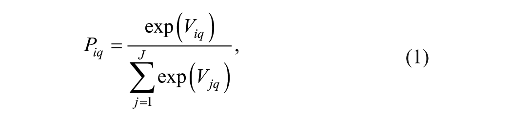
where Piq is the probability that a guest q chooses an alternative i from a set of alternatives where
The MNL model follows directly from the basic axioms of rational choice plus the assumption that the random error term of the expected utility is distributed extreme-value type 1 (Louviere, Hensher, & Swait, 2000; McFadden, 1974). For most practical applications, the deterministic part of the expected utility for a certain alternative (Viq) is defined as an additive, main effects-only function of the attributes, that is,

where, in addition, β
k
is the marginal utility (i.e., part-worth) associated with attribute level k from a set of K attribute levels, and
First, it is proposed to include a series of interaction terms to model the effect of the size of the booking window on the utility of a booking option. More precisely, it is proposed to model the deterministic part of utility as follows:
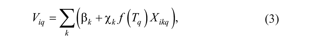
where, in addition, β
k
is the constant (or static) utility parameter associated with attribute level k,
Second, two functional forms for
Heterogeneity
Although conveniently simple, the basic MNL model suffers from some major drawbacks, most importantly the questionable assumptions of “Independence from Irrelevant Alternatives” (IIA) and homogeneity of tastes. IIA is the property that the presence or absence of an alternative in a choice set does not affect the ratio of the probabilities associated with the other alternatives in that choice set (Louviere et al., 2000). Although this assumption greatly simplifies many aspects of model estimation, it is at the same time very restrictive. For example, it is questionable whether a high-priced, luxurious hotel will draw market share proportionally from another high-priced, luxurious hotel versus a cheap, low-standard hostel—an effect that would be predicted by the standard MNL model. In reality of course, one would expect similar propositions to compete more closely with one another than with propositions that are less similar. Also, the MNL assumption that all consumers share the same average taste weights (β
kq
= β
k
for all
One way of dealing with these challenges is to use a mixed logit model, also known as a random coefficients multinomial logit (RCMNL) model. In RCMNL,
Design
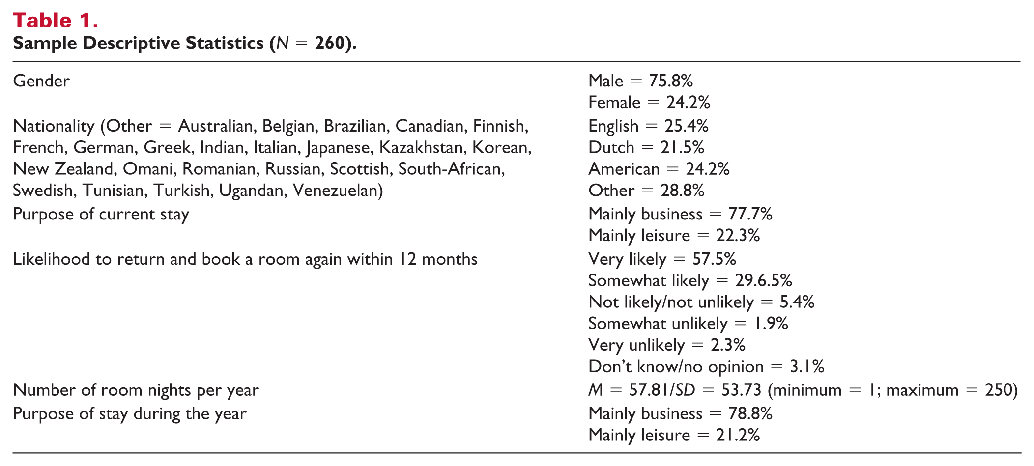
An empirical study to demonstrate the proposed model was undertaken in collaboration with a leading global hotel chain. A total of 260 computer-aided personal interviews (CAPI) were carried out in the lobbies of three of the chain’s properties in the Netherlands. Descriptive statistics are provided in Table 1.
Sample Descriptive Statistics (N = 260).
The interviews were conducted by front office personnel on i-Pads and took about 10 min for the actual hotel guests to complete. Sawtooth Software SSI Web 8 was used as the interviewing platform. A screenshot of one of the stimuli is illustrated by Figure 1. Both English and Dutch questionnaires were available to the respondents.

Screenshot of a Typical Choice Task Used in the Study.
A number of observations should be made about the setup of these choice tasks. First of all, both the name of the properties in the first sentence and the hotels’ standard room description were conditioned on the actual hotel property where the respondent was staying (established through a previous survey question). This was done to make the questionnaire as relevant as possible for each individual respondent. Second, one could observe the variable number of days prior to arrival stated in red (i.e., the size of the booking window: T), which varied over the choice tasks. The levels used for T where 2 days, 7 days, 14 days, 30 days, and 60 days. As can be seen, the respondents were primed to consider an overnight stay throughout the week. This was done because the majority of the hotels’ clientele were business guests, and consequently, the fieldwork was always conducted on working days. Third, it can be seen that every choice task contained two booking alternatives with varying rate conditions and prices. The conjoint analysis design thereby contained four attributes: three binary (on/off) attributes for the rate conditions (i.e., free cancelation, free date change, and pay on departure) and one price attribute varying on five levels (€185, €200, €215, €230, €245) representing actual standard room rates. By clicking on the blue “i” buttons, the respondent was able to activate pop-ups containing detailed information on the rate conditions. These conditions, as well as their descriptions, were taken directly from the actual hotel chain under study. Finally, every choice task included a “no-choice” option to establish a threshold utility for choice suspension (Vno-choice = βno-choice).
Every respondent received a total of 10 choice tasks in which the attribute levels were varied according to a random stimulus design generated by SSI Web, thus effectively creating a unique choice design for every individual respondent. The 10 choice tasks for every respondent were then grouped into five sets of two choice tasks each. Each of these sets was associated with one of the five booking window levels in descending order (so 60, 30, 14, 7, and 2 days, respectively). This was done because a purely random ordering of the booking windows across the choice tasks was perceived as to result in too much of a “chaotic” experience for the respondent, potentially resulting in inconsistent choices. A descending order of the booking windows (instead of ascending) was felt to be the most coherent with the feeling of a “natural flow of time.” Every subset of choice tasks was preceded by a text screen to prime the respondent for a particular booking window.
As the likelihood function of the RCMNL model did not have a closed-form expression, the model estimation proceeded numerically through simulation. The statistical software package BioGeme (Bierlaire, 2003) was used for this purpose with the application of 150 Halton draws per respondent to achieve stable results within acceptable runtimes (Train, 1999). Bhat (2001) pointed out that using 125 Halton draws will yield about the same level of reliability as using 2,000 random draws, and this is empirically consistent with Train (1999) and Zeng (2016). Both also show that in terms of reliability, little can be gained by using more than 100 Halton draws. To simulate the results for analysis, Microsoft Excel was used with 10.000 “simulated” guests to obtain stable results. Price was coded as a single scalar for parsimony (i.e., “linear attribute coding”).
Results
Table 2 presents the estimated parameters and significance tests for the time-independent benchmark model (RCMNL), the proposed model with a linear specification for the booking window, Model 1: f(Tq) = Tq / 10, and the proposed model with a logarithmic specification for the booking window, Model 2: f(Tq) = ln(Tq). The benchmark model is a standard RCMNL model with constant means and standard deviations for the price coefficient, the three binary coefficients for the rate conditions (free cancelation, free date change, pay on departure), and the no-choice constant. The model has a significantly higher explanation than a null model (log likelihood [LL] ratio = 1,287.6, p < .01; adj. ρ2 = .222). All estimated means are significant (p < .01) and have expected signs and relative magnitudes, indicating that all the attributes shown in the choice task have an effect on the aggregate choice behavior of the respondents. However, only one of the five estimated standard deviations (for price) is significant (p < .01), indicating that consumers seem to be fairly homogeneous in their sensitivity toward the rate conditions.
Estimated Parameters for the Benchmark and Proposed Models.
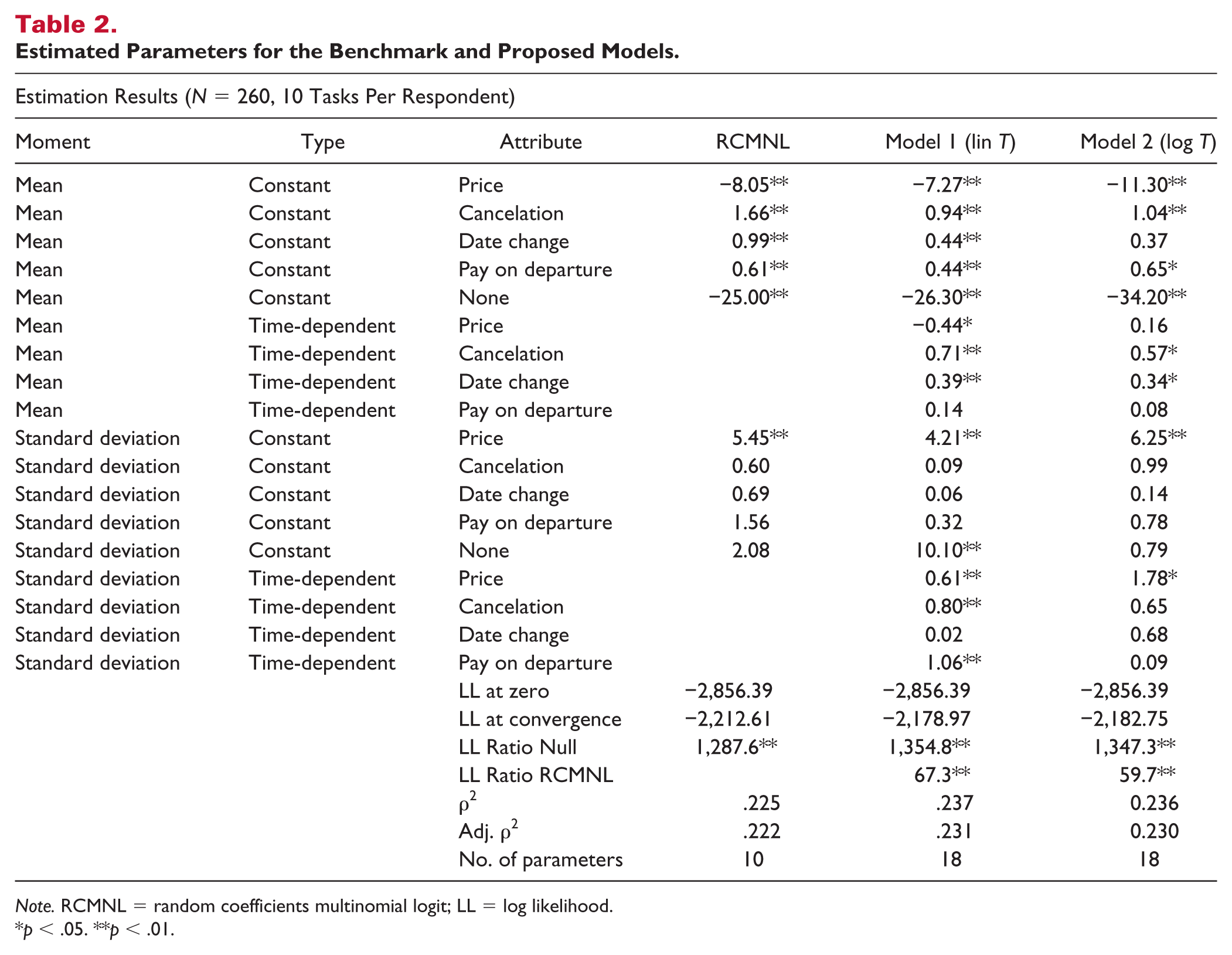
Note. RCMNL = random coefficients multinomial logit; LL = log likelihood.
p < .05. **p < .01.
Models 1 and 2 offer a higher explanation than the null model (Model 1: LL ratio = 1,354.8, p < .01, adj. ρ2 = .231; Model 2: LL ratio = 1,347.3, p < .01, adj. ρ2 = .230). Moreover, both models offer a significantly higher explanation than the benchmark model (Model 1: LL ratio = 67.3, p < .01; Model 2: LL ratio = 59.7, p < .01). The results suggest that the linear (i.e., constant impatience) specification for the booking window, perhaps due to the limited 60-day time window (akin to Park & Jang, 2014), provides a better fit than the logarithmic (i.e., decreasing impatience) specification and can be chosen as the final model.
While all constant mean components are significant predictors of choice (p < .01), Model 1 also shows strongly significant and positive time-dependent mean components for cancelation and date change (p < .01). This indicates that the ability to cancel or change the date on a booking is indeed preferred more when the booking window increases. Of the two rate conditions, free cancelation is more sensitive to the size of the booking window than free date change, which seems rational as cancelation involves a higher potential financial risk than a date change. The sensitivity to pay on arrival is significant as well, albeit not related to the size of the booking window. An interaction effect between free cancelation and free date change was considered but did not result in a significant contribution within Model 1 (constant: t = 1.35, p = .18 & time-dependent: t = 1.04, p = .30) or Model 2 (constant: t = 0.65, p = .52 & time-dependent: t = 1.33, p = .18).
A closer inspection of the estimated standard deviations of the time-dependent effects suggests that guests are quite heterogeneous in the degree to which their preference for price, cancelation, and pay on departure vary over time. For date change, time-varying preferences are more consistent across guests. The fact that pay on departure has an insignificant time-dependent mean but significant time-dependent standard deviation indicates that although there is some variation in time-dependent preferences over booking agents, these average out at near zero across the sample.
Practical Illustration
A common application in conjoint analysis would be to calculate WTP from any set of conjoint utilities that include a scalar monetary attribute (most typically room price) by simply dividing the utility of the rate condition by the negative of the scalar price utility (i.e., the marginal utility of a one-Euro price increase). That is,

However, as pointed out by Orme (2001) as well as Ofek and Srinivasan (2002), this notion of WTP is naïve, as the formulation does not take the dependency on other rate attributes or competitor rates into account. Also, as pointed out by Scarpa, Thiene, and Train (2008), the formulation in Equation 4 may lead to extreme values when calculated on an individual respondent basis, as small values for βprice in the denominator may result in extremely large WTP values for rate conditions which may render aggregation useless.
Ofek and Srinivasan (2002) suggest the “Market Value of an Attribute Improvement” (MVAI) as an alternative measure for the WTP. That is,
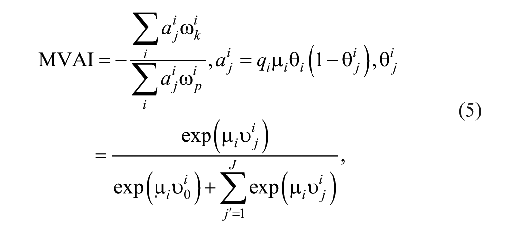
where
The calculation of MVAI in practice would require the revenue manager to provide a complete specification of the choice set. Using the empirical study of this note, the choice set could be (a) a standard room with no rate conditions at €215 (i.e., average for all properties) plus (b) a “no-choice” option. Table 3 shows the MVAI values for the three rate conditions at varying booking windows, together with the WTP values derived from Equation 4, and the manually determined MVAI (MDMVAI) values following the approach of Orme (2001).
MVAI for Rate Conditions at Different Booking Windows.
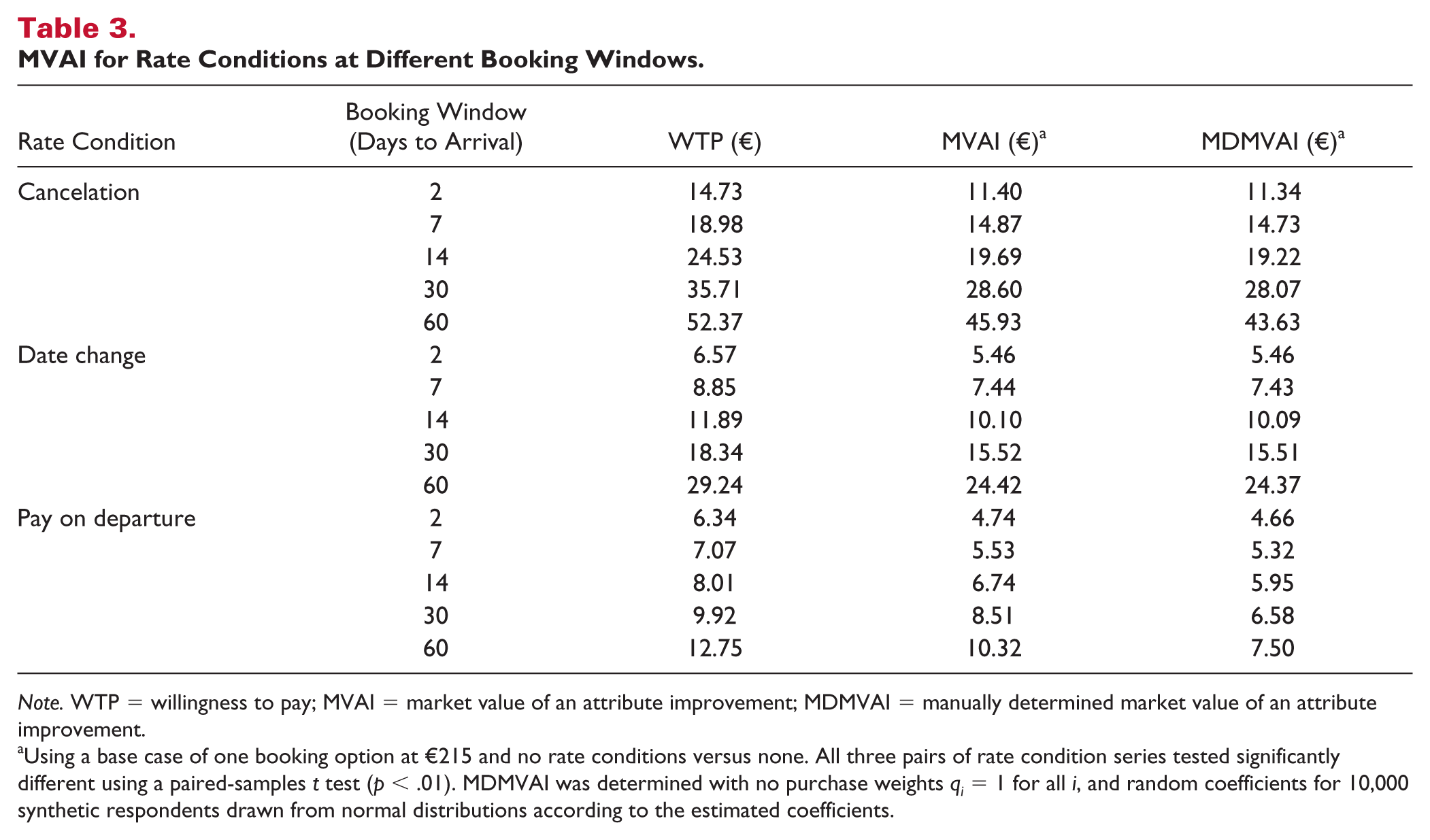
Note. WTP = willingness to pay; MVAI = market value of an attribute improvement; MDMVAI = manually determined market value of an attribute improvement.
Using a base case of one booking option at €215 and no rate conditions versus none. All three pairs of rate condition series tested significantly different using a paired-samples t test (p < .01). MDMVAI was determined with no purchase weights qi = 1 for all i, and random coefficients for 10,000 synthetic respondents drawn from normal distributions according to the estimated coefficients.
It shows that the MVAI for cancelation, with its significant time-varying utility parameter, quite strongly depends on the size of the booking window. With only 2 days between booking and arrival, the average guest is willing to pay only €11.40 for the ability to cancel, which gradually increases to €45.93 at a 60-day booking window. Thus, the bigger the booking window, the more consumers are willing to pay for the ability to cancel the booking (without penalty). The same general result applies to date change, although the effect is less pronounced. Both at 2 days (€5.46) and at 60 days (€24.42), the WTP is approximately half that of cancelation. The premium for pay on departure is the least affected by the size of the booking window (from €4.74 at 2 days to €10.32 at 60 days), which is illustrative for the fact that the time-dependent utility parameter for this rate condition is not significant. The results are graphically depicted in Figure 2.
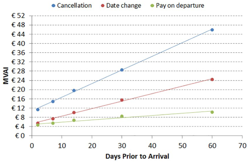
MVAI at Different Booking Windows for all Rate Conditions.
Discussion and Limitations
Answering to a call for the exploration of a dynamic pricing approach for rate conditions (Chen & Xie, 2013), this research note demonstrates how conjoint analysis can be applied to examine consumer preferences and sensitivities for rate conditions over the booking horizon. It thereby draws attention to a novel CBC model modification by which preferences can be predicted as a function of time. This choice model includes time as an additional “attribute.” The attribute is not a feature of the choice propositions, but instead is associated with the choice context. Given a lack of systematic empirical research on temporal aspects of buying behavior in revenue management (Chen & Schwartz, 2008), tourism (Park & Jang, 2014), and marketing (Garcia & Ruiz, 2016), this can be considered a significant method contribution.
Several studies have found that hotel guests’ WTP is greater when the booking window shortens (e.g., Abrate & Viglia, 2016; Guizzardia, Ponsa, & Ranieri, 2017; Guo, Ling, Yang, Li, & Liang, 2013; Schamel, 2012; Schwartz, 2000; Su, 2007). As rate conditions can be viewed as a price attribute (e.g., a surcharge for the option to cancel without penalty), they impact WTP. This was demonstrated in research on advanced booking policies (e.g., Chen et al., 2011; Schwartz, 2000, 2006, 2008; Smith et al., 2015), for example, in the context of consumer search and deal-seeking booking behavior. Methods to analyze time-dependent choice behavior thus have significant implications for hotel revenue management practice. This research note suggests that stated choice data can be used to empirically derive WTP figures for the rate conditions for any specific booking window. When these data are enriched via integration with revealed preference data, and combined or compared with multiple sources of stated choice and preference data (Louviere et al., 2000), modified time-dependent choice models can be used by revenue managers in practice to determine the conditioned and unconditioned room rate structure over the booking horizon by analyzing the potential increase of revenue when rate conditions are priced dynamically as compared with a static/fixed surcharge set for each unconditioned room rate (e.g., penalty-free cancelation) in relation to the corresponding conditioned room rate.
Although all significant effects had expected directions (i.e., no parameter reversals) despite a limited sample size, providing evidence of the robustness of the model, it should be noted that a convenience sample was used for this study, which consisted mainly of business guests who may not have been the actual booking agents. The guests thus could have been be less price-sensitivity than leisure guests or professional booking agents. The three hotels under study were notably business oriented as was confirmed by the fact that 77.7% of all respondents reported to stay mainly for business purposes. Data were available on whether respondents described their visit as mainly for business (n = 202) or mainly for leisure (n = 58), yet the fact that no questions were included in the questionnaire on whether respondents made the booking themselves (at their own expenses) can be regarded as a major shortcoming of the research. As a general indication of whether price sensitivity would differ between business and leisure guests, Model 1 was separately estimated for both groups. The results indicate that the price sensitivity indeed was lower for business than for leisure guests, t(258) = 10.81, p < .01. Interestingly, also the price attribute showed some sensitivity to time (p < .05). This unanticipated result might be indicative of the fact that guests may associate shorter booking windows with capacity constraints, although this was not specifically stated in the choice tasks. This finding and the development of a methodology—akin to De Palma, Picard, and Waddell (2010)—to address room availability limitations (i.e., constrained capacity) in discrete choice modeling are important issues for future research. To this purpose, upscale cruising could provide a rather good industry setting for empirical testing. First, it would reduce the number of control variables as the customer base is less segmented. Second, the luxury cruise industry is much more consolidated. Therefore, decisions over rate conditions are much more driven by WTP than by market share. Third, the cruise industry has much stricter and much more complex cancelation policies, with a whole secondary market for insurance plans, given that the financial stakes are much higher. In this context, multistage regression could be considered as during the booking window alternative travel experiences may be available, assurance plans may vary, and cruise lines may offer promotions at any given point in time.
Footnotes
Declaration of Conflicting Interests
The author(s) declared no potential conflicts of interest with respect to the research, authorship, or publication of this article.
Funding
The author(s) received no financial support for the research, authorship, or publication of this article.