
Abstract
Background:
Recent development of automated closed-loop (CL) insulin delivery systems, the so-called artificial pancreas (AP), improved the quality of type 1 diabetes (T1D) therapy. As new technologies emerge, patients put increasing trust in their therapeutic devices; therefore, it becomes increasingly important to detect malfunctioning affecting such devices. In this work, we explore a new paradigm to detect insulin pump faults (IPFs) that use unsupervised anomaly detection.
Methods:
We generated CL data corrupted with IPFs using the latest version of the T1D Padova/UVA simulator. From the data, we extracted several features capable to describe the patient dynamics and making more apparent suspicious data portions. Then, a feature selection is performed to determine the optimal feature set. Finally, the performance of several popular unsupervised anomaly detection algorithms is analyzed and compared on the identified optimal feature set.
Results:
Using the identified optimal configuration, the best performance is obtained by the Histogram-Based Outlier Score (HBOS) algorithm, which detected 87% of the IPF with only 0.08 false positives per day on average. Isolation forest is the best algorithm that offers more conservative performances, detection of 85% of the faults but only 0.06 false positives per day on average.
Conclusion:
Unsupervised anomaly detection algorithms can be used effectively to detect IPFs and improve the safety of the AP. Future studies will be dedicated to test the presented method inside dedicated clinical trials.
Keywords
Introduction
The introduction of continuous glucose monitoring (CGM) devices1,2 and continuous subcutaneous insulin infusion (CSII) pumps has considerably improved the quality of care for patients with type 1 diabetes (T1D). 3 Furthermore, recently developed automated closed-loop (CL) insulin delivery systems, the so-called artificial pancreas (AP), 4 have shown clear potential to further improve the quality of glucose control while simultaneously reducing the requested actions for the patient, thus partially relieving them from the burden of the disease. Other recent technologies, such as CGM sensors that do not require calibrations, 5 smart insulin bolus calculators,6-11 possibly based on computer vision-based carbohydrate estimators, 12 aim at further reducing the amount of actions required from the patients, to improve their quality of life.
As new technologies help patients with T1D to worry less about their disease, patients tend to put more and more trust on them. 13 Therefore, it becomes increasingly important to detect possible malfunctioning affecting such systems. Insulin pump faults (IPFs) are the most critical source of hazard for the safety of patients with T1D in pump therapy, 14 including AP users. 15 Problems with CSII can be caused by mechanical defects 16 or kinking, occlusion, and displacement from site è.17,18 When unrecognized, IPFs typically lead to hyperglycemia and ketonemia.19,20 It is also observed that problems with pumps are one of the main factors that contribute to diabetic ketoacidosis (DKA).21-24
In this paper, we deal with the problem of automatically detecting IPFs and we focus in particular on an AP setup. In this context, highly informative data collected by the device can be used for detection: CGM sensor measurements, patient provided meal announcements, and injected insulin information (including both patient manual corrections and modulations performed by the controller).
Automatic methods for the detection of IPFs aim to warn the patient of the malfunctioning to decrease hyperglycemia excursions and DKA incidence. Traditionally, this problem was investigated using model-based fault detection techniques.25-30 In this approach, a mathematical model of the patient is identified and then used to predict blood glucose (BG) values using meal announcements and injected insulin information. The predicted values are continuously compared with CGM measurements and a fault is detected when a large difference between the two is observed. Unfortunately, to identify an accurate model capable of capturing the large inter- and intra-subject variability observed in T1D subjects can be very challenging.
Recently, in a proof-of-concept work, 31 we explored a new paradigm to detect IPFs, alternative to model-based methods and relying on unsupervised AD algorithms. These algorithms, developed by the machine learning community, aim at identifying the anomalies (faulty data, incorrect measures, or outliers) in a dataset, by means of supervised or unsupervised approaches. Supervised AD algorithms require a training set, containing examples of normal data and anomalies. These data are called labeled data because a teacher/supervisor has classified (labeled) them in a proper way. By looking at these examples, the algorithm learns the properties that distinguish normal data from anomalies. Once this “learning” procedure is completed, the algorithm uses the learned criteria to classify a new data as anomaly or normal. Unsupervised AD algorithms, instead, do not require labeled data, but are based only on the observation of past examples of data (historical data): new data are detected as anomaly if they differ significantly from data previously observed. Unsupervised AD is applied in many applications, for example, in network intrusion detection, fraud detection, and medical science.32,33
Using unsupervised algorithms is especially useful in the case of IPF detection, since data where the functioning/faulty status of the pump is accurately known are hard to collect in practice. This can be done either via dedicated experiments or through retrospective visual inspection performed by an expert operator. Unfortunately, the second procedure is highly time consuming and prone to errors.
Aim of the Study
This work expands the proof-of-concept proposed in Meneghetti et al 31 by addressing the open issues:
(i) Dealing with a crucial step in the anomaly detection pipeline: The definition of an effective feature set, ie, suitable numerical attributes capable to describe the status of a patient and effective in making IPFs detectable. This will be done by considering many possible features, possibly defined ad hoc, and selecting the most effective ones.
(ii) Comparing the performance of several different anomaly detection algorithms available in the literature to identify the most suitable ones for our purpose.
(iii) Investigating a hybrid approach that blends anomaly detection and model-based methods, by including among the considered feature set the prediction residuals obtained using personalized predictive models identified using single patients’ data.
Methods
Dataset
To assess the fault detection algorithms, a dataset containing information on the beginning and duration of the faults to be used as ground-truth is needed. Accurate collection of such data requires dedicated experiments, which are hard to perform in practice also because of safety reasons. Alternatively, clinical data can be visually inspected by a human operator to label suspicious data portion likely affected by an IPF. Unfortunately, this procedure is time consuming and prone to errors. Finally, another option is to use simulated in silico data instead of real ones, since this permits to have perfectly accurate ground-truth labels without performing potentially harmful experiments on real patients.
In this paper, we resort to the last option. In silico data are obtained using the latest version of the Padova/UVA T1D simulator. 34 Compared to the previous version, 35 this version of the simulator includes new features that increase the realism of the testing scenario: intraday variability of insulin sensitivity, time-varying distributions of the patients’ therapy parameters, and a model of “dawn” phenomenon. 36 Using all the 100 adult virtual subjects of the simulator, we simulated 30 days of CL therapy, using a proportional integral derivative (PID) controller. 37 Three meals per day were simulated (breakfast, lunch, and dinner), taking place with uniform probability at [7:30, 8:00], [12:00, 13:30], and [19:00, 20:30]. The amount of carbohydrates assumed in each meal was randomly sampled from a uniform distribution with mean and SD derived from data published in Brazeau et al 38 (58.2 ± 22.5 g for breakfast, 77.7 ± 27.0 g for lunch, and 83.9 ± 32.3 g for dinner). We also simulated carb-counting errors made by patients as modeled in Vettoretti et al. 39
Two pump faults per patient were simulated in 30 days, similar to the frequency reported in van Bon et al. 40 One fault occurs at midnight of a random day, while the other at noon of another day. Both days are selected independently, with uniform distribution over 30 days of simulation. The first episode checks the ability to detect a fault at fasting and the second the ability to detect an episode even if occurring during postprandial glucose increase. During the IPF, insulin injection is interrupted for a duration of six hours. After this time, we assume that the fault is noticed by the patient and insulin injection is restored through manual intervention. It is of little interest to consider faults lasting more than six hours, since after six hours we declare an unsuccessful detection (see the “Evaluation Criteria” section).
Three simulated datasets are obtained using different seeds of the random number generator, which decides the random parameters of the simulation. The first dataset (training set 1) is used to perform the feature selection procedure. The second dataset (training set 2) is used to find the optimal algorithm hyperparameters and the third dataset (test set) is used to test the unsupervised AD algorithms on data never observed before.
Evaluation Criteria
To evaluate the algorithms, we performed a segmentation of each of the three 30 days datasets obtained from each virtual patient, into portions of six hours, starting from 00:00 of the first day. Two of these portions completely contained the IPFs, since they take place at noon or at midnight of a random day and have a duration of six hours.
If at least an alarm is raised in the IPF portions, a true positive (TP) is assigned, if not a false negative (FN) is assigned. For all the other portions, if an alarm is (wrongly) raised, a false positive (FP) is assigned, if not a true negative (TN) is assigned. Finally, since pump faults cause the system to remain in an anomalous state for some time after the fault is restored, the six-hour time window after the fault is not considered in the evaluation. In this way, possible late alarms occurring in that portion are not counted as FP. Similarly, even if no alarm is raised in that portion, the TN count is not increased.
The dataset is heavily imbalanced: two IPF segments every 30 × 24/6 = 120 segments per patient. Therefore, to assess the performance, the metrics of precision and recall (also known as sensitivity) are calculated:

Specificity is instead of limited interest. 41 Since the number of false positives (FPs) is expected to increase as the length of the experiment increases, we also calculate the average number of FPs per day (FP/day) in the population.
Insulin Pump Fault Detection Method Design
In Figure 1, on the left side, the IPF detection method steps are illustrated. As a first step, CGM sensor measurements, meal announcements, and insulin injection information are collected during the patient’s use of the system. At each time step, the incoming data are processed and numerical features describing patient status (eg, glucose rate of change or Insulin On Board) are computed. This step is known as feature extraction. Then, the obtained features are fed to the unsupervised AD algorithm, which produces an anomaly score that measures how much the new data differ from the other previously observed ones. The specific criteria employed to assign the score vary from one AD algorithm to the other. When the anomaly score exceeds a threshold, an alert is generated to warn the patient of a possible IPF.
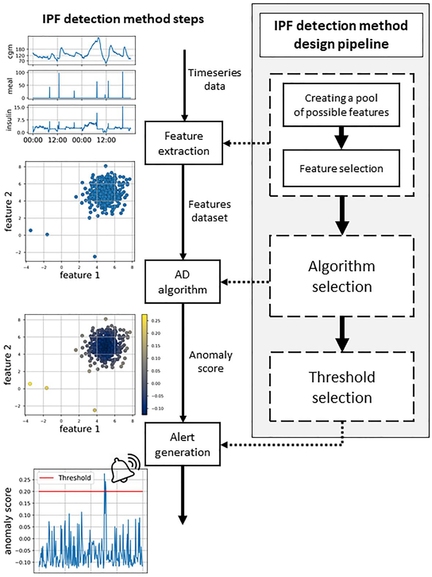
Scheme of the insulin pump fault detection method steps (on the left) and the design pipeline (on the right).
Figure 1 also shows, on the right side, the pipeline that is followed to design the proposed IPF detection method. The first step is to consider several possible features that have the potential to highlight the anomalous state of the patient induced by IPF. Subsequently, we select the most effective ones by discarding redundant or ineffective features (feature selection step). Then, we comprehensively compared the unsupervised AD algorithms available in the literature and select the most effective ones to detect IPFs. Finally, the threshold to be applied to the anomaly score for the generation of the alarm is selected. In the following, we discuss in detail each of these design steps.
It should be noted that the first two design steps (the definition of the optimal feature set and the selection of the optimal algorithm) need to be performed independently from the choice of the threshold that is made only as a last step. To do so, in the first two steps, the performance will be investigated using the Precision-Recall curve that is obtained by considering different threshold values on the anomaly score for the generation of the alarm.
Creation of a pool of possible features
In this section, we define a large pool of possible features, potentially capable of describing the status of the patient and highlight IPFs. Later, in the feature selection procedure, the optimal feature set will be defined.
At each time step t, we considered as a possible feature, describing the status of patient, the current CGM value (cgm(t)), and the derivative of the CGM signal, obtained using a high-pass filter (der(t)), or the linear fit of the CGM data (slope(t)) (see Appendix for more details). To capture a common symptom of IPFs, hyperglycemia, we calculated the time that a patient spends above two different threshold of glycemic values, 180 mg/dL (t_h180(t)) and 250 mg/dL (t_h250(t)). These last two features are calculated starting from when threshold is exceeded. When the glycemia returns below the threshold, the time is reset.
We also include information on the injected insulin in the descriptors of patient status and, in particular, at each time step t, we consider insulin correction

and representing how much the injected insulin i(t) deviates for
Similar to insulin, we compute the residual carbohydrates, Carbohydrates On Board (cob(t)), as reported in Schiavon et al. 43 An estimate of the amount of carbohydrates in the plasma (pce(t)) can also obtained as the convolution with a second-order filter (see Appendix for details).
We also considered among the descriptors the cross-correlation between CGM and plasmatic insulin (gxi(t)), and between CGM and carbohydrates in plasma (gxc(t)) (see Appendix for details).
Moreover, we included two features that were introduced in Meneghetti et al, 31 specifically crafted for highlighting anomalous behaviors linked with IPFs. The first one, dcob is a weighted version of the glucose derivative, reduced in the presence of a meal:
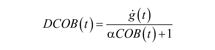
with
The second introduced feature focuses on Insulin On Board: icob is a weighted version of IOB, reduced in the presence of a meal:
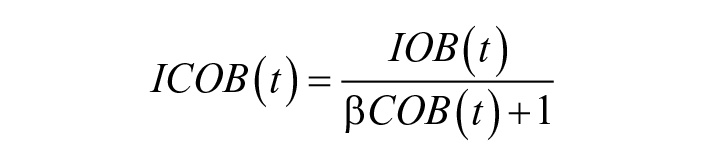
with
Furthermore, we included two quantities proposed by Howsmon et al 44 : Insulin Fault Metric (ifm(t)) and Glucose Fault Metric (gfm(t)). These two quantities aim to highlight considerable deviations of the current values of glucose and plasma insulin as compared to average values in the last 24 hours (see the “Appendix” section).
Finally, we considered some features inspired by model-based fault detection techniques, where measured glucose values are compared with predicted values obtained using a predictive model. A very large difference between the two quantities (prediction residual) is suspicious and likely to be caused by a fault. Therefore, prediction residuals can be considered as additional features. Three different prediction horizons are considered: one hour (pres1h(t)), two hours (pres2h(t)), and three hours (pres3h(t)).
Feature values are normalized using min-max scaling, using minimum and maximum values observed in single patients. All the considered features are summarized in Table 1; more details on the computation are provided in the Appendix.
Pool of Considered Features.
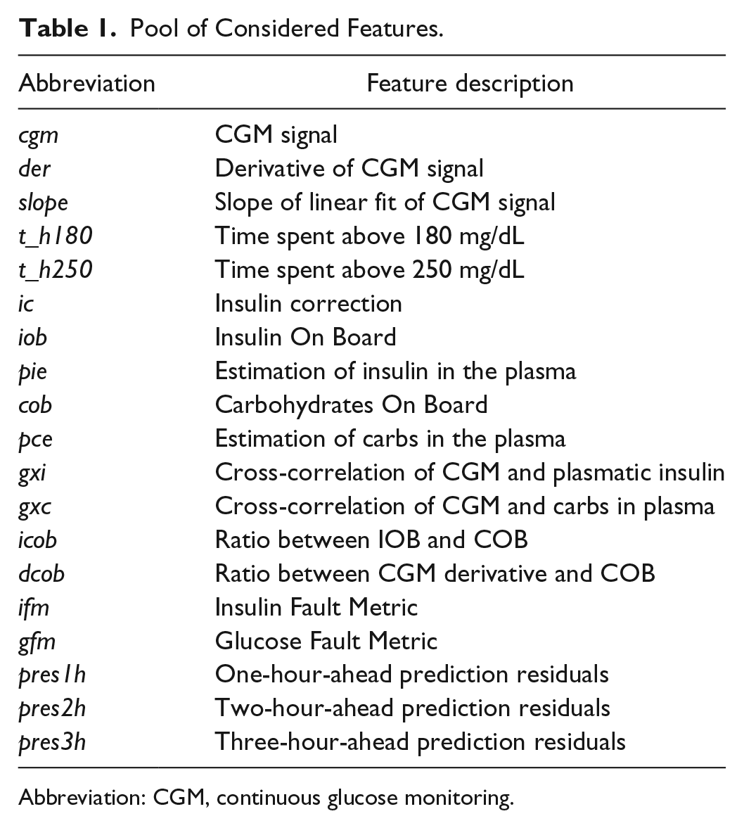
Abbreviation: CGM, continuous glucose monitoring.
Feature selection
To select the optimal feature set, forward and backward feature selection were performed. 45 In forward feature selection, as a first step, each individual feature is tested to select the one that results in the best performance, according to a suitable performance criterion (discussed later). Next, all the possible combinations of the selected feature and a new one are evaluated to select the best second feature. The procedure is repeated by adding features one by one until all of them are considered. Symmetrically, backward feature selection starts by considering all the features and works backward from there, removing one by one the feature that leads to the smallest performance deterioration (the less relevant feature), until no more are left. The importance of a feature can thus be measured by the order in which the feature is selected in the procedures described above.
During the feature selection procedure, the performance improvement/degradation achieved by adding/removing a feature is evaluated using the average precision. Average precision can be interpreted, with a small approximation, as the area under the Precision-Recall curve 41 obtained considering different threshold values for the generation of the alert (see Appendix for details). Figure 2 shows an example of two Precision-Recall curves obtained by two algorithms. In this space, the ideal performances are achieved in the top right corner. Larger areas under the curve thus suggest that algorithm 1 (blue) is more effective for most of the thresholds. The average precision can therefore be used to compare the performance of the algorithms independently from the chosen threshold.
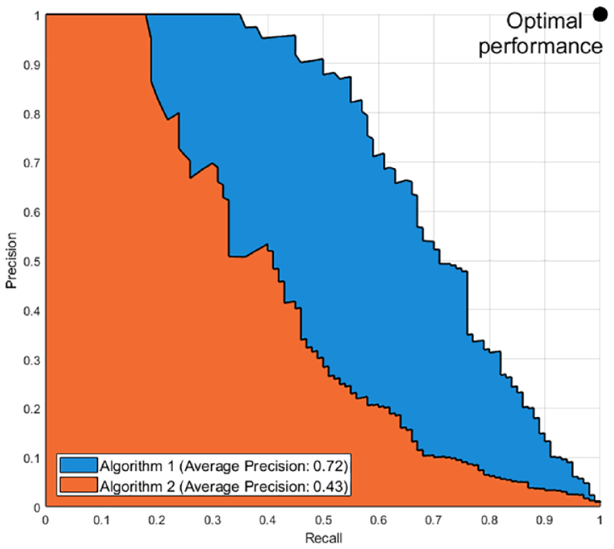
Example of a comparison of two Precision-Recall curves and their respective average precision.
Figures 3-6 show the results of forward and backward selection procedure for the four most relevant AD algorithms in our application (HBOS, IForest, OCSVM, and KNN, see the next section). Analogous behaviors are observed for the other algorithms considered in this paper. The x-axis reports the order in which the features were selected (forward) or removed (backward), from first to last. The y-axis reports the average precision obtained when adding (removing) the corresponding feature in the x-axis.
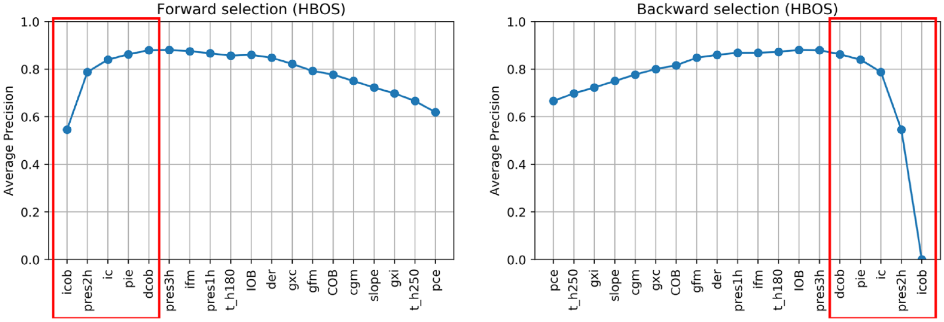
Feature selection on HBOS.
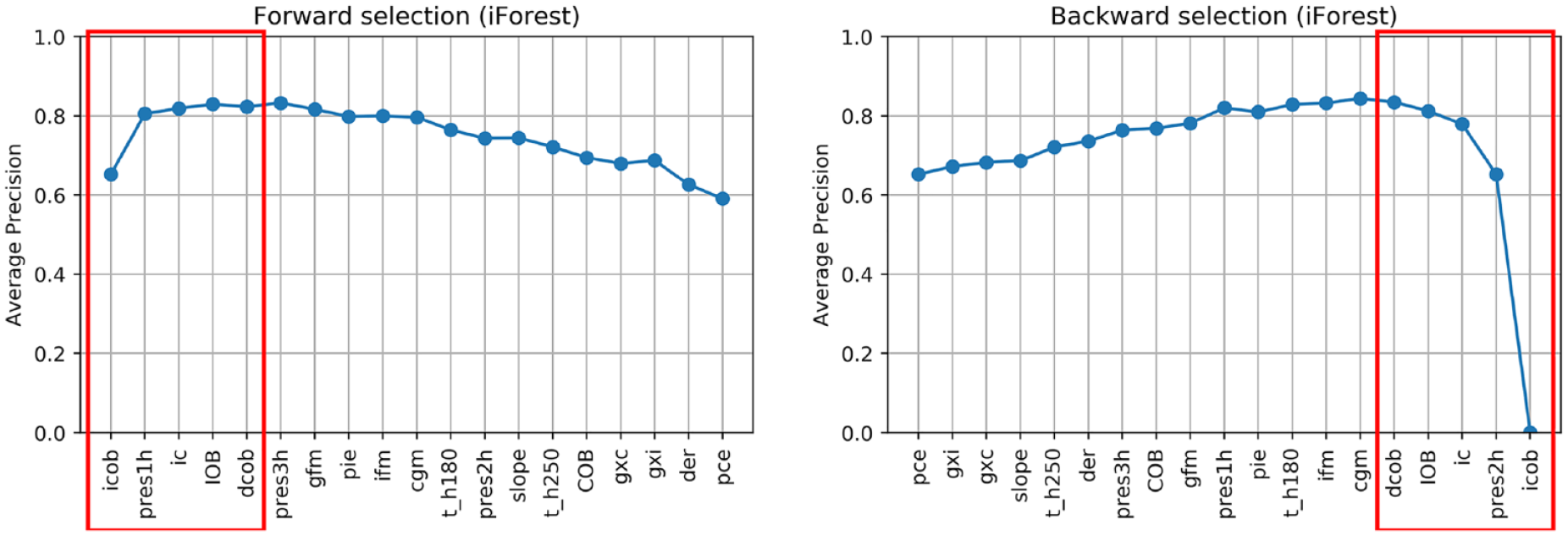
Feature selection on IForest.
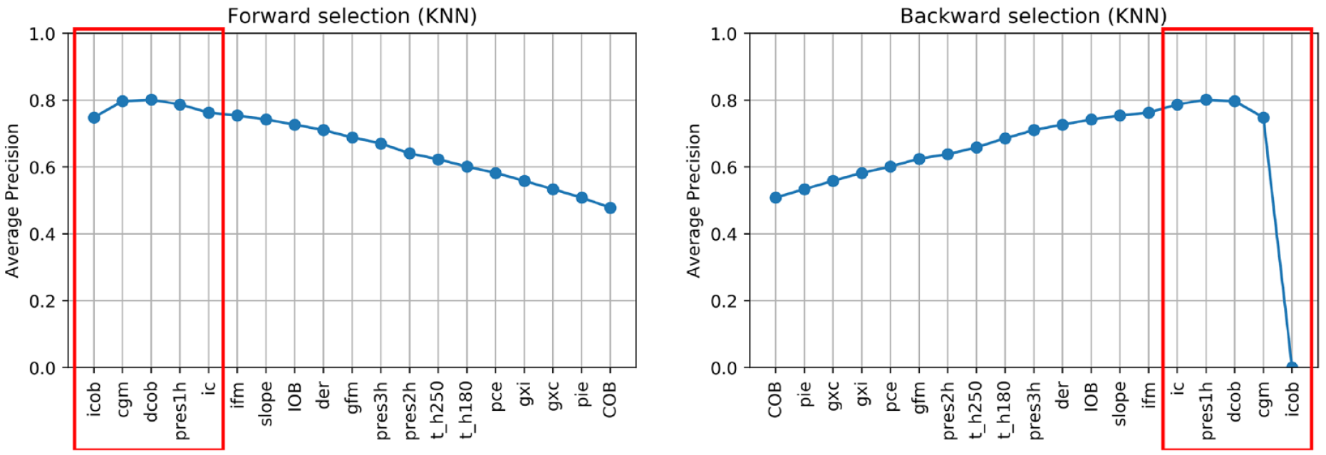
Feature selection on KNN.
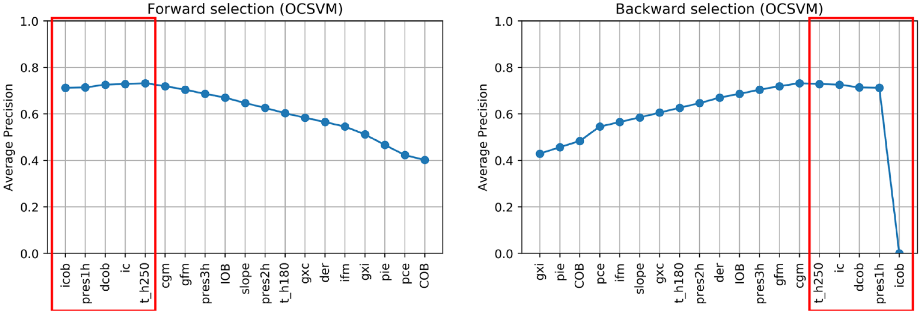
Feature selection on OCSVM.
In all cases, increasing the number of features results in an improvement of the average precision and then, possibly after a plateau, the performance decreases when considering additional features. A good tradeoff for all methods is achieved by using the first five features (highlighted in red). In fact, five features grant optimal performances for OCSVM; minor improvements can be achieved with HBOS and IForest if one or two extra features are added, while with KNN would suggest a more parsimonious feature set.
In all the algorithms, icob and dcob (features specifically crafted aiming to highlight IPF) are among the five most important features. Prediction residuals at one and two hours are also selected in most of the cases among the top five features. Since these two features are highly correlated, one is enough to increase the performance of the algorithms. Choosing one or the other has limited impact on the performances. Nonetheless, since pres2h appears four times, while pres1h appears five times, we opted to select pres1h.
The ic feature is also of clear importance, since it highlights extra insulin injection in the attempt to compensate for hyperglycemia. Finally, KNN and OCSVM benefit from including cgm and t_h250, respectively, two features related to glucose and capable of highlighting hyperglycemia based on CGM readings. Also in this case, the two features are highly correlated, one is enough to improve the performance and the choice of one over the other has limited impact on the performances. Nevertheless, since cgm is chosen in the second place for KNN and is chosen right after t_h250 in OCSVM, we opted to include cgm in our feature set.
In conclusion, icob, dcob, pres1h, ic, and cgm were selected as the optimal feature set to detect IPFs.
Algorithm selection
Various anomaly detection unsupervised AD algorithms have been proposed in machine learning literature, differing mostly on the criteria used to assign the anomaly score. In this work, we tested and compared several of them for our purpose, as summarized in Table 2. The table also reports a reference for each method, where more details can be found. For the implementation of the algorithm we used a distribution that is available at PyOD, 46 an open source library of anomaly detection algorithms, except for osPCA for which we used an ad hoc MATLAB implementation.
Unsupervised Anomaly Detection Algorithms Considered in This Work.
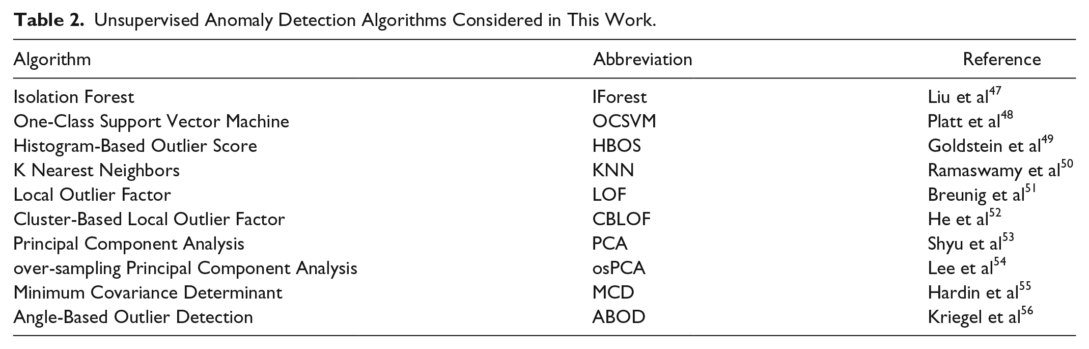
All the algorithms are fed with the optimal feature set discussed above. The algorithm hyperparameters are tuned on the training set 2, by comparing different Precision-Recall curves obtained with each hyperparameter, using the same procedure reported in Meneghetti et al. 31 Supplemental Table S1 in the Appendix reports the values of the hyperparameters selected.
Threshold selection
As a final step of the AD design pipeline, we need to select the anomaly score threshold to generate an alarm. For this task, we focus on average FP/day rather than on precision. In fact, the number of FPs is expected to increase as the length of the experiment increases, thus leading to precision decreases. Since our experiment is relatively long, choosing the threshold based on precision would lead to highly conservative setting.
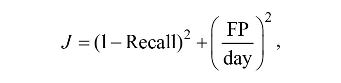
Figure 7 reports the results obtained by each algorithm on the training set 2, in the Recall vs FP/day space. Each curve is obtained for different values of the threshold and colored differently according to the algorithm. In this representation, the optimal configuration is the one closest to the bottom right corner. Therefore, the threshold is selected as the value that minimizes the distance from the said corner:
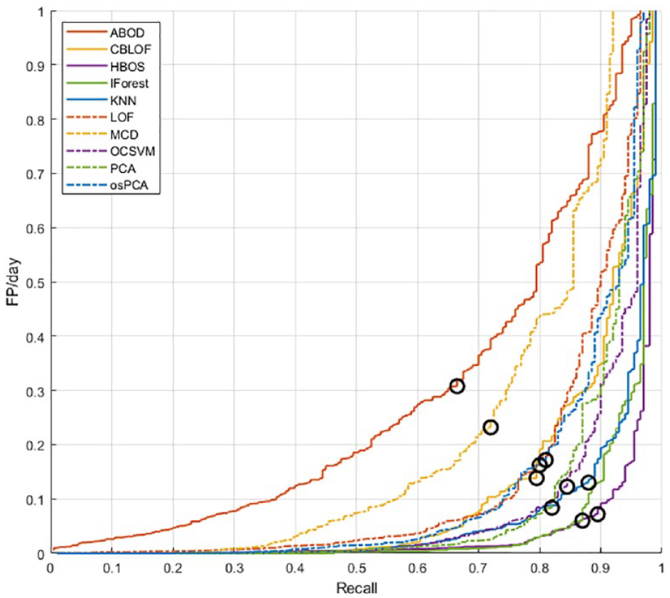
Analysis of the performance obtained in the Recall-FP/day space for the selection of the optimal threshold.
In each curve, we highlighted with a black circle the performance achieved with the optimal threshold.
Supplemental Table S2 in the Appendix reports the final values of the thresholds selected for all algorithms.
Results
Using the optimal feature set identified on training set 1 and the algorithms’ hyperparameters selected on training set 2, we proceeded to test all the algorithms on the test set. In Figures 8 and 9, the Precision-Recall curves and the Recall vs FP/day curves obtained with various AD algorithms are shown.
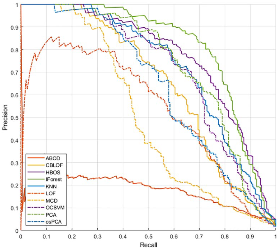
Algorithm comparison in the Precision-Recall space on the test set.
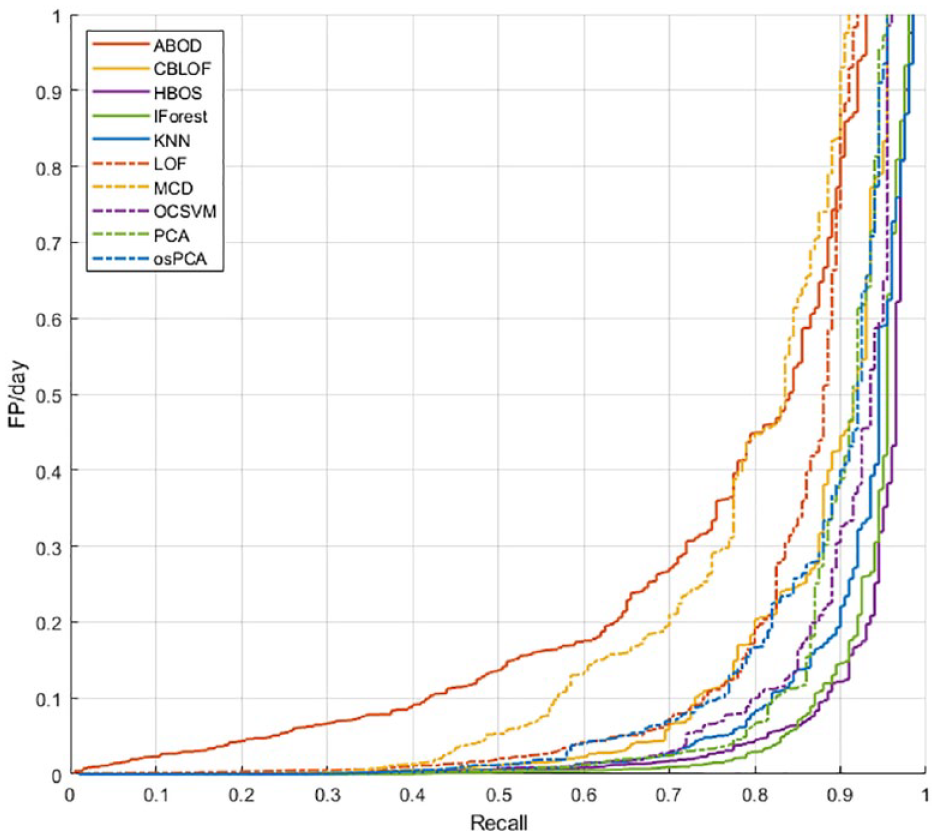
Algorithm comparison in the FP/day-Recall space on the test set.
For all the considered thresholds, IForest and HBOS exhibit the best performance, followed by OCSVM, KNN, and PCA.
Table 3 reports the Recall and the FP/day obtained on the test set by each algorithm, using the optimal threshold, selected using the procedure previously described.
Performance Obtained on the Test Set by all the Unsupervised Anomaly Detection Algorithms Using the Optimal Threshold.
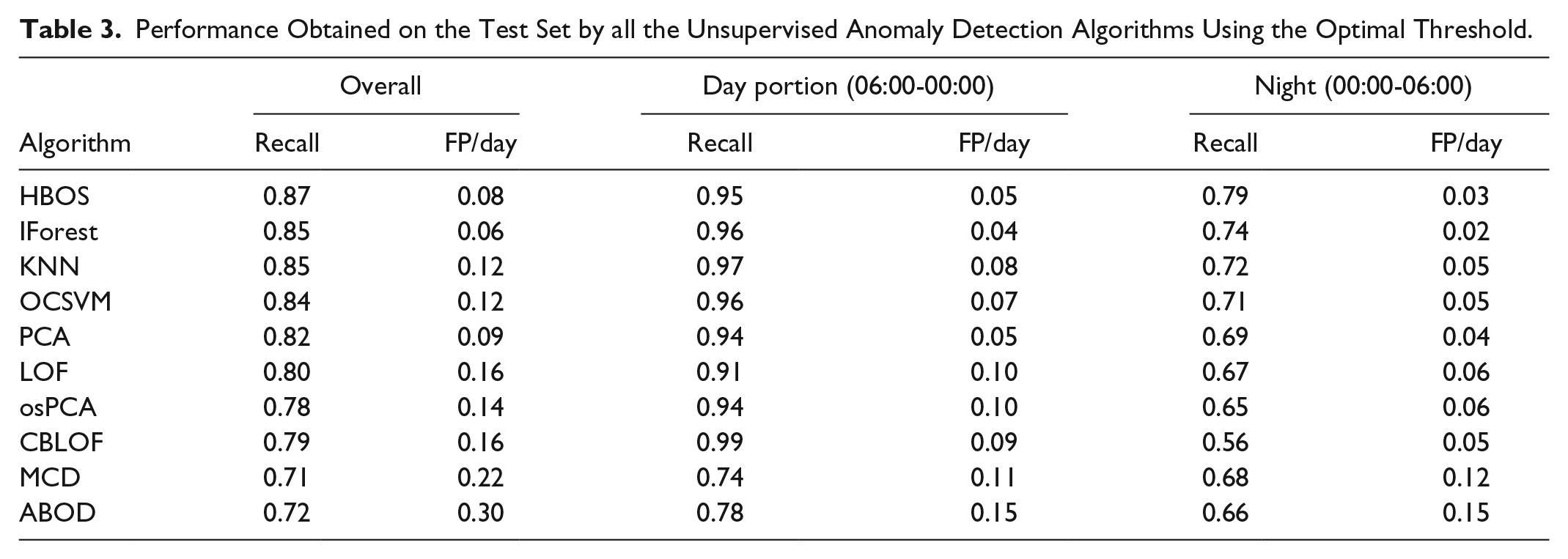
The best recall is obtained by HBOS, which scored a recall of 0.87 with 0.08 FP/day, ie, less than 1 FP every 10 days. Slightly lower recall is achieved by IForest (0.85) but with a relevant reduction of FP/day (0.06). The other methods, instead, are outperformed by these two in at least one of the metrics.
Table 3 reports also the performance analysis focused on day-time (06:00-00:00) and night-time (00:00-06:00) only. Both portions are affected by one pump fault per patient in 30 days: in the latter portion, the episode occurs at fasting, while in the former detection has to be performed during a postprandial peak.
In the overnight period, the picture is similar to the one of the overall period. HBOS achieves the highest recall (0.79) with the second lowest FP/day (0.03), while IForest grants the lowest lower FP/day (0.02) with the second highest recall (0.74). The other methods, instead, are clearly outperformed by these two in at least one of the metrics. During the diurnal portion, the picture is slightly more complicated. IForest still grants the lowest FP/day (0.04) with one of the highest recalls (0.96): the third highest performance, after CBLOF and KNN (0.99 and 0.97, respectively), but these last two methods produce twice ore more the FP/day (0.09 and 0.08, respectively). HBOS show performances slightly inferior to IForest, presenting the second lowest FP/day (0.05, equal to PCA), and the fourth recall (0.95). Also in this case, CBLOF and KNN achieve better recall but at the expenses of a nearly double FP/day ratio. In view of this, HBOS and IForest emerge as the most promising algorithms for this problem.
Notably, these results show that with the proposed approach detecting an insulin pump malfunctioning is harder at fasting than when the patient dynamics are excited by a meal, in spite of the possible confounding effect of postprandial hyperglycemia.
Comparison With State of Art
In this work, we explored an innovative approach to detect IPFs that are based on unsupervised AD algorithms. Previous works in the literature considered different solutions for detecting IPF. One of the most investigated approaches is model-based fault detection. These methods leverage on either black-box personalized linear models25,26 or nonlinear physiological models.27-30 The accuracy of model-based methods is linked to that of the predictive model. Unfortunately, the task of identifying an accurate predictive model is a complex challenge because of the huge inter- and intrasubject variability we observe in patients with T1D. With respect to model-based strategies, our approach does not require to identify an accurate predictive model of the patient physiology.
The problem of detecting IPF can also be casted into a supervised binary classification task, where classes are defined as “fault” or “nonfault,” as proposed in Rojas et al. 57 In this approach, a decision function is fit on labeled data, where precise information about the system functioning (“fault” or “nonfault”) is contained. The possibility of using supervised algorithms is dubious given the limited availability of accurate labeled data. In fact, to obtain such data, a human operator would have to label the data manually via visual inspection, but such procedure can be challenging and prone to errors. Alternatively, a dedicated clinical experiment could be used, but such experiment is hard to perform in practice also because of safety reasons. Finally, labeled data can only be obtained for a subset of patients; therefore, subject-specific data are not available in general. With respect to supervised anomaly detection, our method does not require any labeled data to be trained on.
Finally, two contributions proposed custom algorithms based on the monitoring of specific signals extracted from CGM and CSII data. Cescon et al proposed a method for anticipating rather than detecting IPFs 58 reporting a recall of 0.5 and 0.004 FP/day on a dataset collected from real patients (n = 23). Howsmon et al proposed their method 44 and tested it online on a real clinical trial 59 reporting a recall of 0.88 and 0.22 FP/day, also on a dataset of real patients (n = 25). The results reported in this work, although obtained on simulated data, show that our method outperforms the method of Cescon et al by obtaining a higher sensitivity. Our method also outperforms Howsmon et al by scoring the same recall but halving the false positives. We would like to stress that that these last two methods were tested on a more challenging dataset; therefore, the comparison above is only preliminary and biased in favor of our method. A conclusive comparison should be performed on the same dataset.
Considerations on the Feature Selection Results
Finally, it is interesting to comment on results of the feature selection procedure presented in the “Feature selection” section.
The two features proposed in Meneghetti et al 31 (icob and dcob), specifically crafted for highlighting IPFs resulted in very important features in our method. Insulin correction (ic) also resulted to be a very important feature to monitor. This feature captures the effort to correct for hyperglycemia performed by the controller (or by the patient via manual corrective boluses) and as such is informative on possible IPFs.
We also investigated a possible hybrid approach with model-based fault detection techniques, by including prediction residuals as additional features in the considered pool. These features were selected by the procedure, proving their value in highlighting IPFs. Interestingly, the impact of prediction residuals was particularly important for effective IPF detection after a meal.
We also considered as possible features the quantities proposed by Howsmon et al 44 in their detection algorithms. However, they were not selected before the other features were available.
We also noticed that almost all the features aiming to highlight hyperglycemia, a common symptom of an IPF, are selected later than the other proposed features. A possible interpretation for this is that high values of glycemia (and long periods of hyperglycemia) may occur also without an IPF, because of a nonoptimal meal bolus or simply a large meal. High values of icob, dcob, and ic proved instead to be more tightly related to IPFs.
Adding too many features results in a degradation of performance. This effect is commonly known as curse of dimensionality: 45 when the number of considered features becomes too large, issues may arise, eg, distances becoming numerically similar or too many irrelevant attributes being considered. 60
Limits of This Work
The results presented in this work are obtained on simulated data. The use of simulated data is particularly relevant in fault detection studies: first of all, because they allow to test the impact of faults, possibly very dangerous or extreme ones, without posing them at risk the patient or exposing them to discomfort; moreover, in simulation, the exact timing and duration of the fault is perfectly known; finally, in the simulated scenario, other potentially confounding factor can be canceled. Nevertheless, although the simulator used is the latest and most challenging version of the FDA-approved UVA/Padova simulator (including both inter- and intrasubject variability), simulation is always a largely simplified test case.
Specifically, several simplifications were made, including the assumption of three meals per day and the uniform random time of IPF occurrence. In real-world scenarios, other factors affect the data, including but not limited to unannounced meals, exercise, and day-time or night-time snacks.
To overcome this limitation and perform a more realistic validation of the method propose, our next step will be to challenge the algorithms with real data and to test them in dedicated clinical trials.
Conclusion
The short duration of insulin infusion set is still a major safety hazard for patients with T1D. Although it is recommended that insulin infusion sets are changed frequently (every two to three days), medical surveys reveal that patients fail to stick to the recommended guidelines. 61 Automatic detection of IPF can reduce the patient’s concern about changing the infusion set before malfunctioning occur and, as a result, they can encourage the patients to adhere even more to insulin pump therapy.
In this work, we explore a novel paradigm to detected pump malfunctioning, based on unsupervised anomaly detection techniques. The resulted detection method was tuned and tested using the latest version of the FDA-approved Padova/UVA T1D simulator. A feature selection procedure was performed on a proposed feature set that included features aiming to describe the patient status and highlight anomalies linked to IPFs. A comparison of several unsupervised AD algorithms was also performed to identify the most suitable ones for the application. Furthermore, the inclusion of the prediction residuals in the feature set resulted in improving the performance of the unsupervised AD algorithms.
Using the identified optimal configuration, the best performance is obtained by HBOS, which scored a recall of 0.87 and 0.08 FP/day, ie, roughly 1 FP every 10 days, and by IForest, that offers a more conservative alarm strategy with slightly lower recall (0.85) but lower FP/day (0.06).
Future work, aimed at testing the presented method on real data and in dedicated clinical trials, is envisioned.
Supplemental Material
Binder1 – Supplemental material for Detection of Insulin Pump Malfunctioning to Improve Safety in Artificial Pancreas Using Unsupervised Algorithms
Supplemental material, Binder1 for Detection of Insulin Pump Malfunctioning to Improve Safety in Artificial Pancreas Using Unsupervised Algorithms by Lorenzo Meneghetti, Gian Antonio Susto and Simone Del Favero in Journal of Diabetes Science and Technology
Supplemental Material
dst-19-0142_appendix_revised – Supplemental material for Detection of Insulin Pump Malfunctioning to Improve Safety in Artificial Pancreas Using Unsupervised Algorithms
Supplemental material, dst-19-0142_appendix_revised for Detection of Insulin Pump Malfunctioning to Improve Safety in Artificial Pancreas Using Unsupervised Algorithms by Lorenzo Meneghetti, Gian Antonio Susto and Simone Del Favero in Journal of Diabetes Science and Technology
Footnotes
Declaration of Conflicting Interests
The author(s) declared the following potential conflicts of interest with respect to the research, authorship, and/or publication of this article: L.M, G.A.S, and S.D.F. hold patent applications related to the proposed method.
Funding
The author(s) disclosed receipt of the following financial support for the research, authorship, and/or publication of this article: This work was supported by the Ministero dell’Istruzione, Università e Ricerca (Italian Ministry of Education, Universities and Research) through the project Learn4AP: Patient-Specific Models for an Adaptive, Fault-Tolerant Artificial Pancreas (initiative “SIR: Scientific Independence of young Researchers”, Project ID: RBSI14JYM2).
Supplemental Material
Supplemental material for this article is available online.
References
Supplementary Material
Please find the following supplemental material available below.
For Open Access articles published under a Creative Commons License, all supplemental material carries the same license as the article it is associated with.
For non-Open Access articles published, all supplemental material carries a non-exclusive license, and permission requests for re-use of supplemental material or any part of supplemental material shall be sent directly to the copyright owner as specified in the copyright notice associated with the article.