Sage Journals: Discover world-class research

Abstract

Background:

An essential component of any artificial pancreas is on the prediction of blood glucose levels as a function of exogenous and endogenous perturbations such as insulin dose, meal intake, and physical activity and emotional tone under natural living conditions.

Methods:

In this article, we present a new data-driven state-space dynamic model with time-varying coefficients that are used to explicitly quantify the time-varying patient-specific effects of insulin dose and meal intake on blood glucose fluctuations. Using the 3-variate time series of glucose level, insulin dose, and meal intake of an individual type 1 diabetic subject, we apply an extended Kalman filter (EKF) to estimate time-varying coefficients of the patient-specific state-space model. We evaluate our empirical modeling using (1) the FDA-approved UVa/Padova simulator with 30 virtual patients and (2) clinical data of 5 type 1 diabetic patients under natural living conditions.

Conclusion:

Compared to a forgetting-factor-based recursive ARX model of the same order, the EKF model predictions have higher fit, and significantly better temporal gain and J index and thus are superior in early detection of upward and downward trends in glucose. The EKF based state-space model developed in this article is particularly suitable for model-based state-feedback control designs since the Kalman filter estimates the state variable of the glucose dynamics based on the measured glucose time series. In addition, since the model parameters are estimated in real time, this model is also suitable for adaptive control.

Keywords

artificial pancreas type 1 diabetes glucose Kalman filter identification empirical model

Diabetes mellitus is a group of metabolic disorders in which blood glucose concentration is elevated, wholly or in part due to failure of pancreatic insulin secretion. Left untreated, hyperglycemia can result in acute complications and can also chronically result in multiorgan dysfunction, including blindness, kidney failure, and cardiovascular disease. Insulin therapy has been shown to delay the onset and progression of diabetes-related complications for type 1 diabetes. In the past decade, much progress has been made in the development of a mechanical “artificial pancreas” (AP), which would be a wearable (or implantable) automated insulin delivery system consisting of a continuous glucose monitor (CGM), an insulin pump, and a control algorithm closing the loop between glucose sensing and insulin delivery.¹

The development of an AP is a challenging task. One of the major challenges lies in that the biochemical and physiologic kinetics of insulin and glucose are complex, nonlinear, and only approximately known. Several so-called compartmental models based on glucose fluxing between different “compartments” in the body have been proposed.^2-4 More recently, empirical models for glucose dynamics have also been pursued in the literature.^5-19

Most of the existing empirical models for glucose prediction use glucose measurements only. For example, an impulse response model based on an orthogonal basis function was identified.² An AR model was identified based on continuous glucose data of 9 type-1 diabetic patients with data-shooting and regularization techniques to improve the performance of parameter estimation.⁵ The effects of insulin or meal intake on glucose can be included in the empirical models by introducing exogenous (X) input variables, though the effect of meal input on glucose has been much less commonly explored than the effect of insulin, since most models in the literature have been developed for fasting conditions.^6,7 Based on fingerstick measurements of glucose obtained from ambulatory data of a single subject, Ståhl and Johansson examined various black-box models such as ARMA, ARMAX, subspace, transfer function, and nonlinear ARMAX models.⁸ Finan et al evaluated the performance of several empirical models, such as zero-order hold and ARX models, identified from diabetic patient data in ambulatory conditions.⁹ Recent work on glucose prediction has also explored inputs of insulin and meal intake, as well as other factors such as exercises and stress levels.^10-12

Recursive least squares (RLS) algorithms have been more dominant than nonrecursive algorithms in identifying model parameters in recent literature. Some early articles using RLS for parameter estimation were reviewed by Hovorka,¹³ and more recent research included estimation of coefficients of AR or ARMA models,^14-16 ARX models,⁹ and ARMAX models.^10,17 Recently, neural network (NN) models for glucose predictions have been studied in several articles.^12,18,19 It was noted that NN-based models not necessarily outperform simple time-series models such as low-order AR models.¹² Zecchin et al developed a new NN-based model, which was used in parallel with a linear predictor and augmented with a physiological model of glucose rate of appearance in plasma, and claimed that this approach performs better than a first-order AR model.¹² However, the proposed NN model was not compared to any ARX models with insulin or meal intake as inputs.

In this article, we develop a new data-driven approach for modeling glucose dynamics of type 1 diabetic patients, accounting for both effects of insulin and meal intake. Our new strategy involves the use of a phenomenological dynamic state-space model with time-varying model coefficients. Then corresponding to each individual type 1 subject, a recursive estimation based on extended Kalman filtering (EKF) is applied to estimate the time-varying parameters and the state variable of the dynamic model (glucose concentration) simultaneously. Developing a time-varying empirical model, in contrast to the linear time-invariant black-box models in the literature, could potentially overcome uncertainties associated with the modeling of insulin/meal-glucose kinetics, and allow the instantaneous re-estimation of model parameters. Kalman filtering has been used to denoise CGM sensor data in several articles.^20
-24 For example, a Kalman filter was used to estimate denoised CGM profile and predict glucose levels by modeling the glucose dynamics as a double-integrator (in terms of the derivative and the second derivative of glucose) with no insulin or meal as input variables.^20,21 Kalman filtering was also used with smoothing criteria,²² and within a Bayesian calibration method,²³ to increase the accuracy of CGM. To the best of our knowledge, this article is the first in the diabetes literature to apply EKF to estimate the glucose level and time-varying model parameters of glucose dynamics simultaneously. Besides the aforementioned advantages in denoising the CGM sensor data and real-time estimation of time-varying model coefficients, EKF also provides prediction of error covariances of the glucose concentration and model parameters, which could be potentially used to reduce false alerts of hypo-/hyperglycemia, as well as for robust control system designs.

In this article, we evaluate our empirical models using (1) an FDA-approved simulator with 30 patients consisting of 10 adults, 10 adolescents, and 10 children and (2) normal free-living diabetic patient data of 5 type 1 subjects, consisting of continuously monitored time series of glucose concentration, insulin dose, and meal intake.

Methods

In this section, we first propose a data-driven state-space model to characterize the dynamics of glucose with time-varying parameters, based on continuously monitored glucose, insulin dose, and meal intake. Then an EKF is applied to estimate the time-varying model coefficients, for which the filter consistency of EKF can be checked using statistical tests.

Time-varying State-space Model for Glucose Dynamics

Let t = 0, 1, . . . , T denote the discrete-valued time index, where the invariant interval between consecutive times could be arbitrary. At each time t, let z(t) denote the measured blood glucose, x(t) the insulin delivered, and y(t) the carbohydrate being taken. We consider the following linear time-varying model for glucose dynamics,

z (t) = ζ (t) + n (t)

(1)

ζ (t + 1) = Φ_{t} [ζ (t)] + B_{t} [x (t - v)] + Γ_{t} [y (t - w)] + ε (t)

(2)

where the measured blood glucose z(t) at each time t is decomposed into the true blood glucose ζ(t) (corresponding to the interstitial fluid CGM sensor data z(t), ζ(t) denotes the interstitial glucose concentration) and measurement error n(t). In addition, the true level of blood glucose ζ(t+1) at time (t+1) is a function of process noise ϵ(t) and the following 3 components,

Φ_{t} [ζ (t)] = ϕ_{1} (t) ζ (t) + ϕ_{2} (t) ζ (t - 1) + \dots + ϕ_{p} (t) ζ (t - (p - 1))

(3)

B_{t} [x (t - v)] = β_{1} (t) x (t - v) + β_{2} (t) x (t - v - 1) + \dots + β_{q} (t) x (t - v - (q - 1))

(4)

Γ_{t} [y (t - w)] = γ_{1} (t) y (t - w) + γ_{2} (t) y (t - w - 1) + \dots + γ_{r} (t) y (t - w - (r - 1))

(5)

where $Φ_{t} [ζ (t)]$ denotes an autoregressive component of order p, explaining the blood glucose at time (t+1) in terms of a linear combination of p time-lagged values of blood glucose: ζ(t−i), i = 0, 1, . . . , p−1. $B_{t} [x (t - v)]$ denotes a dynamic linear regression of the blood glucose at time (t+1) on q time-lagged values of insulin delivery: x(t−v−i), i = 0, 1, . . . , q−1, with v ≥0 denoting a fixed delay. $Γ_{t} [y (t - w)]$ denotes a dynamic linear regression of the blood glucose at time (t+1) on r time-lagged values of meal intake: y(t−w−i), i = 0, 1, . . . , r−1 with w ≥ 0 denoting a fixed delay.

An important innovative feature is that the autoregressive coefficients $ϕ_{k} (t), k = 1, 2, \dots, p;$ dynamic regression coefficients $β_{k} (t), k = 1, 2, \dots, q;$ and $γ_{k} (t), k = 1, 2, \dots, r$ can be time-varying in arbitrary ways except that they are assumed to be slow varying. The time varying coefficients and the blood glucose will be estimated simultaneously by an EKF, based on the observed time series (z(t), x(t), y(t)) from initial time to the present time. In the implementation of EKF estimation of the model parameters, we restrict the dynamic regression coefficients $β_{k}$ to be negative and $γ_{k}$ to be positive for all k, because insulin always reduces glucose concentration while carbohydrate always increases glucose concentration.

FIR Modeling of Subcutaneous Insulin Absorption and Meal Absorption

The time delay before subcutaneous insulin acts on glucose level, and the time delay before meal intake affects blood glucose are modeled through a normalized finite impulse response (FIR) function given by (6). Then the insulin dose x(t) and carbohydrate intake y(t) used in the model (2) are given by multiplying the nominal (ie, recorded) insulin dose and estimated carbohydrate intake with their respective FIR.

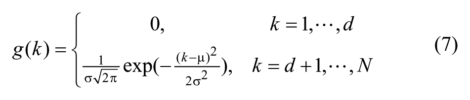
Let G(k), k = 1, . . . , N, denote a FIR function, where k denotes index to sampling intervals, and N denotes the total span of the FIR function in terms of sampling intervals. Considering a dead time of d time intervals, the FIR function G(k) can be represented as follows,

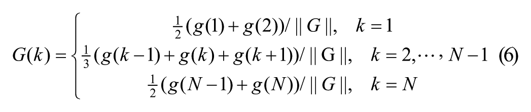
G (k) = {\begin{matrix} \begin{matrix} \frac{1}{2} (g (1) + g (2)) / | | G | |, & k = 1 \end{matrix} \\ \begin{matrix} \frac{1}{3} (g (k - 1) + g (k) + g (k + 1)) / | | G | |, & k = 2, \dots, N - 1 \end{matrix} \\ \begin{matrix} \frac{1}{2} (g (N - 1) + g (N)) / | | G | |, & k = N \end{matrix} \end{matrix}

(6)

where ||G|| denotes the norm of G and 1-norm is used here (other norms could be used as well), and g(k), k = 1, . . ., N, representing a truncated Gaussian distribution with mean denoted by μ and standard deviation denoted by σ, satisfies

g (k) = {\begin{matrix} 0, & k = 1, \dots, d \\ \frac{1}{σ \sqrt{2 π}} \exp (- \frac{{(k - μ)}^{2}}{2 σ^{2}}), & k = d + 1, \dots, N \end{matrix}

(7)

Different parameters for the FIR such as the time span N, dead time d, mean μ and standard deviation σ for the Gaussian distribution can be used to model the patient-specific subcutaneous insulin absorption and meal digestion. A sample FIR with parameters of 5-minute sampling time, 3-hour span (N = 36), dead time d = 4, μ = 12, and σ = 9 is illustrated by Figure 1.

Figure 1.

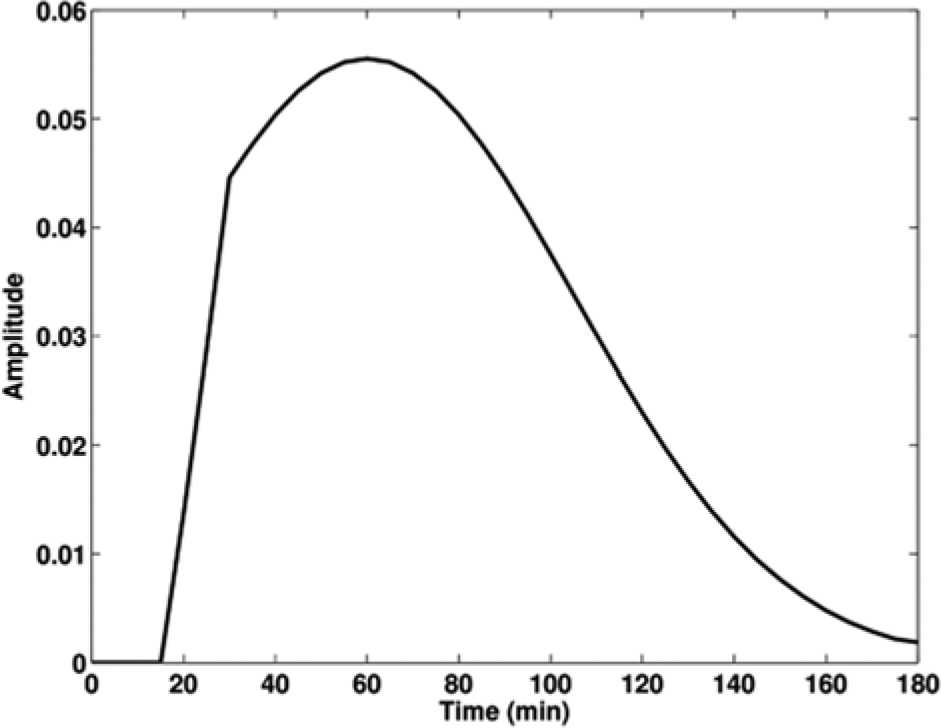
An example finite impulse response (FIR) function used to model subcutaneous insulin absorption or meal absorption; different time span, dead time, and other parameters can be chosen to model insulin and meal absorption, respectively.

Then the insulin dose x(t) and carbohydrate intake y(t) entering (2) are defined in terms of their respective measured values, $x^{m} (t)$ and $y^{m} (t),$ as follows:

x (t) = G (d) x^{m} (t - d) + G (d + 1) x^{m} (t - d - 1) + \dots + G (N) x^{m} (t - N)

(8)

y (t) = G (d) y^{m} (t - d) + G (d + 1) y^{m} (t - d - 1) + \dots + G (N) y^{m} (t - N)

(9)

Since time delay in insulin and meal absorption is captured by the dead time of their respective FIR functions, when (8) and (9) are applied, the fixed delays v and w in (4) and (5) are set to zero (as are the delays v and w in (14) and (15)).

Note that the time varying parameters $β_{k} (t), k = 1, 2, \dots, q;$ and $γ_{k} (t), k = 1, 2, \dots, r$ in (4) and (5) will reshape the insulin and meal effect on blood glucose, and thus the specific values of G(k) in the FIR are not as important as the mean and spread of the Gaussian distribution used in (7).

Physiological models of glucose absorption in terms of glucose rate of appearance (Ra) have been developed in the literature,^25-28 which can be appended to the compartmental models of glucose subsystem and insulin subsystem for the whole-body model of glucose kinetics. Evaluation was conducted by Dalla Man et al,²⁵ and it was claimed that their model outperforms the model by Lehman and Deutsch²⁶ and the one by Elashoff et al.²⁷ Note that the glucose absorption models by Dalla Man et al use population parameters of either normal people or type 2 patients.^25,28 Furthermore, in the context of a personalized AP, the glucose rate of appearance of individual patient is often not measured due to the complicated procedure of tracer-to-tracer ratio clamp technique. Hence, identifying patient-specific parameters of a physiological glucose absorption model^25,28 becomes difficult if not impossible. On the other hand, with the availability of measurement data of glucose concentration, we can directly conduct system identification on the dynamic relation from carbohydrate intake to the glucose concentration without resorting to the intermediate Ra variable. In this article, the dependence of glucose concentration on carbohydrate intake is characterized by the combination of an FIR and real-time estimation of the patient-specific dynamic regression coefficients $γ_{k} (t), k = 1, 2, \dots, r$ . To facilitate understanding, a term referred to as “rate of FIR filtered carbohydrate contribution” is defined in terms of the model in (2) and is compared to Ra in Appendix C.

Our empirical modeling has the following advantages: (1) the combination of FIR and the time-varying dynamic regression coefficients (which are estimated in real time for each subject) allows patient-specific characterization of insulin-glucose and carbohydrate-glucose relationship, (2) the number of parameters needed for estimating a model (based on (4) and (5)) with FIRs is reduced significantly compared to a regression model without using FIRs, for example, for a 3-hour-span carbohydrate FIR (N = 36 for 5-minute sampling time) and q = 6 in (5), a total number of 9 parameters are needed, in contrast to 42 parameters ( $γ_{1}, γ_{2}, \dots, γ_{42}$ ) that would be needed without FIR, to model glucose variation due to the carbohydrate intake 3.5 hours ago.

Extended Kalman Filter to Estimate the Time-varying Coefficients and Glucose Level Simultaneously

Let $Θ (t)$ denote the vector containing all the autoregressive and dynamic regression coefficients

Θ (t) = {[ϕ_{1} (t), \dots, ϕ_{p} (t), β_{1} (t), \dots, β_{q} (t), γ_{1} (t), \dots, γ_{r} (t)]}^{T}

(10)

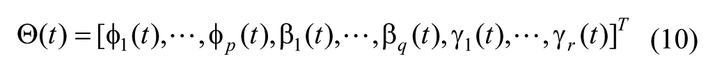
and assume that $Θ (t)$ satisfies

Θ (t + 1) = Θ (t) + ν (t)

(11)

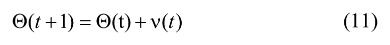
where the stochastic parameter drift ν(t) is described by a white noise drift vector with zero mean and covariance matrix $Q_{v} (t) .$ Then augmenting existing state variables in (2) with the time-varying coefficients $Θ (t)$ gives the extended state variables (or augmented state variables) as follows:

ζ^{e} (t) = {[ζ (t), \dots, ζ (t - p + 1), Θ^{T} (t)]}^{T}

(12)

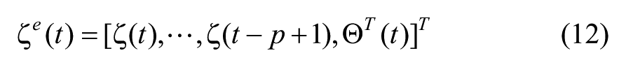
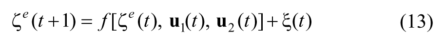
Based on (2) and (11), the augmented state equation can be written as

ζ^{e} (t + 1) = f [ζ^{e} (t), u_{1} (t), u_{2} (t)] + ξ (t)

(13)

where $u_{1} (t)$ denotes the q×1 vector of insulin delivery sequence with

u_{1} (t) = {[x (t - v), x (t - v - 2), \dots, x (t - v - q + 1)]}^{T}

(14)

and $u_{2} (t)$ denotes the r×1 vector of meal intake sequence with

u_{2} (t) = {[y (t - w), y (t - w - 2), \dots, y (t - w - r + 1)]}^{T}

(15)

The explicit form of the nonlinear function f[.] is given in Appendix A. The augmented process noise becomes $ξ (t) = {[ε (t), ν^{T} (t)]}^{T}$ . By assuming that ϵ(t) in (2) is a white noise with zero mean and covariance $Q_{ε}$ , and that ν(t) is a white noise with zero mean and covariance $Q_{ν}$ , we consider the augmented process noise ξ(t) to be a white noise with zero mean and covariance $Q_{ξ}$ . The augmented model (13) is now a nonlinear state equation. It is well known that an EKF can be used for suboptimal state estimation for nonlinear dynamic systems. In this article, we apply a second-order EKF^29,30 to the augmented model (13) for simultaneous estimation of the glucose concentration and the time-varying model coefficients. A brief summary of the second-order EKF is given in Appendix B, and computation of the Jacobian and Hessian of the nonlinear function f[.] needed for the EKF is given in Appendix A. A Kalman filter can also be used as a predictor for glucose in future time steps, and the covariance prediction beyond the time of the last available measurement can be computed as well.²⁹

Consistency of the Extended Kalman Filter

For estimating the state of a dynamic system or estimating a time-varying parameter, convergence of the EKF cannot be guaranteed. Thus the consistency of the filter is evaluated in terms of whether the actual error covariance is consistent with the filter/estimator calculated error covariance. Define the normalized innovation squared (NIS), $ψ = τ (t) ’ S {(t)}^{- 1} τ (t)$ , where the innovation $τ (t)$ is defined as the difference of the measurement and the filter predicted measurement, $τ (t) = z (t) - \hat{z} (t | t - 1)$ , and S(t) denotes the filter calculated innovation covariance. If the filter is consistent, the normalized innovation squared has a chi-square distribution with $n_{z}$ degree of freedom, with $n_{z}$ denoting the dimension of the measurement. To reduce the variability in NIS, real-time consistency can also be evaluated by considering the time-average normalized innovation squared obtained in a single-run test, $\bar{ψ} = \frac{1}{T} \sum_{t = 1}^{T} τ (t) ’ S {(t)}^{- 1} τ (t)$ . If the innovation is white and has a zero mean, $T \bar{ψ}$ has a chi-square distribution with $T n_{z}$ degrees of freedom. In summary, whether the filter is considered consistent is determined by checking if the (time-average) normalized innovation squared falls within the probability concentration region of a chi-square random variable. For example, considering a 1-sided 95% probability concentration region, a single-run real-time test overT time steps for $n_{z} = 1$ requires that $T \bar{ψ} \in [0, χ_{T}^{2} (0.95)]$ , where for T > 100, $χ_{T}^{2} (0.95) = 0.5 {(1.64 + \sqrt{2 T - 1})}^{2}$ .²⁹

Model Evaluation Metrics

Two goodness-of-fit metrics are used to evaluate the prediction performance: coefficient of determination R² and relative absolute difference RAD.³¹ R² indicates the proportion of variability in a data set that is accounted for by a model and thus measures how well future outcomes are predicted by the model,

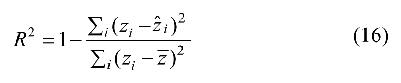
R^{2} = 1 - \frac{\sum_{i} {(z_{i} - {\hat{z}}_{i})}^{2}}{\sum_{i} {(z_{i} - \bar{z})}^{2}}

(16)

where ${\hat{z}}_{i}$ denotes model prediction and $\bar{z}$ denotes mean of the measurements. RAD computes the normalized absolute error between the measurement and prediction with respect to the measured value. At the ith time step, RAD(i) is defined as

R A D (i) = | \frac{z_{i} - {\hat{z}}_{i}}{z_{i}} | \times 100 %

(17)

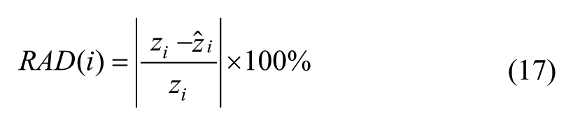
The mean of RAD(i) over the entire simulation period is denoted by RAD.

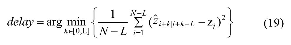
The third metric used to evaluate the glucose prediction is temporal gain (TG),¹² which indicates the amount of average time gained for early detection of a possible hypo/hyperglycemia event using the model. For a sampling time δt(min), a total of N samples, and a L-step ahead prediction horizon, TG (min) is defined as,

T G = (L - d e l a y) * δ t

(18)

d e l a y = \arg \min_{k \in [0, L]} {\frac{1}{N - L} \sum_{i = 1}^{N - L} {({\hat{z}}_{i + k | i + k - L} - z_{i})}^{2}}

(19)

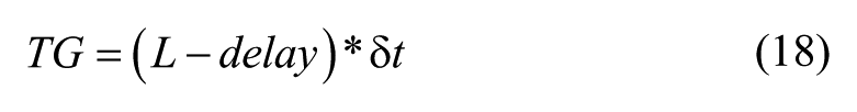
For example, the zero-order-hold prediction scheme (which was used as a comparison basis by Finan et al⁹) has TG = 0, and thus is not useful from a clinical perspective.

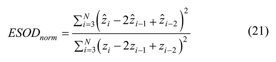
We also evaluate the glucose prediction using a J index,³² which was defined to give a measure of the effective usability of the predicted glucose profile (lower J indicates better prediction), especially in early detection of the ascending and descending trends of glucose and early detection of hyper-/hypoglycemia. J is defined in terms of the ratio of regularity of the predicted glucose profile and the temporal gain,

J = \frac{E S O D_{n o r m}}{T G_{n o r m}}

(20)

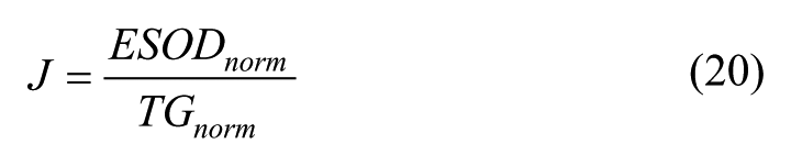
where, $T G_{n o r m} = T G / L$ and ESOD_norm, referred to as the energy of the second-order difference, denotes the normalized sum of the squared second-order differences of predicted time series,

E S O D_{n o r m} = \frac{\sum_{i = 3}^{N} {({\hat{z}}_{i} - 2 {\hat{z}}_{i - 1} + {\hat{z}}_{i - 2})}^{2}}{\sum_{i = 3}^{N} {(z_{i} - 2 z_{i - 1} + z_{i - 2})}^{2}}

(21)

In the end, sensitivity and false alarm rate to detect early hypoglycemia will be computed for a 30-minute prediction horizon and hypoglycemia threshold of 70 mg/dl. A L-step ahead prediction of hypoglycemia is considered false positive if the measurement is actually above the threshold, and considered true positive if otherwise; the prediction of hypoglycemia is false negative when hypoglycemia occurs but not predicted, true negative when alarm is correctly not issued (ie, hypoglycemia does not occur and no alarm being issued). Then sensitivity = true positive/(true positive + false negative) and false alarm rate = false positive/(false positive + true positive).

Data Base

FDA-approved UVa/Padova T1DM Simulator and Virtual Subjects

The training version of the FDA-approved UVa/Padova T1DM simulator^28,33 has 30 virtual subjects consisting of 10 adolescents, 10 adults, and 10 children. The virtual subjects of the simulator were sampled from the experimentally observed intersubject variability. Each virtual subject corresponds to a specific set of parameters, which are totally unknown to the users. In our simulations, we choose the 1-day scenario of the simulator, which simulates blood glucose variation of each virtual subject for 24 hours starting from midnight, with breakfast of 45 g carbohydrate served at 7 am, lunch of 70 g at noon, a snack of 5 g at 4 pm, dinner of 80 g at 6 pm, and another snack of 5 g at 11 pm. Each of the 30 virtual subjects has his/her own individual basal insulin delivery rate. Meal bolus delivered are 3 U for breakfast, 4.7 U for lunch, 5.3 U for dinner. The default sampling time of the simulator is 1 minute. Our model uses a 5-minute sampling time, and thus the data from the simulator were sampled and recorded every 5 minutes.

Free-living Type 1 Diabetic Patient Data

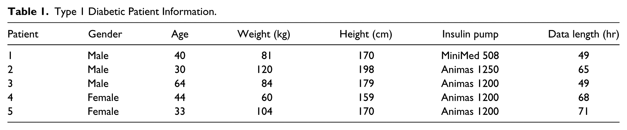
The study protocol for collecting free-living type 1 diabetic patient data was approved by the Institutional Review Board of the Pennsylvania State University. For a 5-minute sampling interval, uninterrupted time series of interstitial glucose concentration measurements, insulin delivery and meal intake were obtained from 5 patients with type 1 diabetes given in Table 1. The patients were not directed to behave in any specific way but rather were encouraged to follow their usual lifestyle. They also followed their own processes for glucose management. As is apparent from the recorded glucose values, these patients were not selected for achieving particularly tight glucose control. Information about insulin dose was obtained by downloading data from the insulin pumps. All patients used analog lispro insulin. Insulin delivery used for modeling was “integrated” and translated into units delivered within 5-minute sampling windows. The MiniMed Continuous Glucose Monitor model MMT-7102 was used to measure interstitial glucose levels, following the standard manufacturer’s directions for sensor insertion and calibration. Macronutrient intake was estimated from digital photographs by a GCRC dietitian, and then entered into Nutritionist Pro Version 4.0.1 (Axxya Systems) to provide estimates per meal/snack of carbohydrate, as well as other macronutrients.

Table 1.

Type 1 Diabetic Patient Information.

Patient	Gender	Age	Weight (kg)	Height (cm)	Insulin pump	Data length (hr)
1	Male	40	81	170	MiniMed 508	49
2	Male	30	120	198	Animas 1250	65
3	Male	64	84	179	Animas 1200	49
4	Female	44	60	159	Animas 1200	68
5	Female	33	104	170	Animas 1200	71

Results

Model Parameters

Following model parameters were used in simulations in this article: p = 2 for the order of the autoregressive component in (3), q = 6 and r = 6 for the order of the dynamic linear regression components in (4) and (5), respectively. The choice of p = 2 is comparable to the order of AR(2) in existing literature for autoregressive components. The choice of q andr together with the FIR length determines the model memory of glucose variation due to insulin and carbohydrate. The parameters for the insulin FIR were chosen to be: N = 24, d = 6, μ = 18, σ = 9; the parameters for the carbohydrate FIR were chosen to be N = 18, d = 1, μ = 3, σ = 6, for all virtual subjects and real patients. Values of these parameters were initially selected based on existing literature on subcutaneous insulin absorption^34,35 and food absorption²⁶ and then retuned using training data. Considering q = 6 and r = 6 and the parameters of the FIRs, the proposed model characterizes glucose changes due to meal intake 2 hours ago and due to insulin administered 2.5 hours ago. We observed that using higher values for p, q, and r did not increase the prediction performance substantially.

In running the EKF, the initial estimates of the model coefficients were chosen as follows: ${\hat{ϕ}}_{1} (0 | 0) = 0.8,$ ${\hat{ϕ}}_{2} (0 | 0) = 0.2,$ ${\hat{β}}_{i} (0 | 0) = - 0.833,$ and ${\hat{γ}}_{i} (0 | 0) = 0.33$ , $i = 1, \dots, 6 .$ All ${\hat{β}}_{i}$ values were constrained to be negative and all ${\hat{γ}}_{i}$ values were constrained to be positive during the iterations, by applying a projection algorithm³⁶ (a summary of the projection algorithm is given in Appendix B). The process noise covariance corresponding to each autoregressive coefficients, $φ_{1}$ and $φ_{2}$ , was chosen to be 0.1% (1%) of its respective initial estimate for virtual subjects (real patients). The process noise covariance for each dynamic linear regression coefficient, $β_{i}$ and $γ_{i}$ , was chosen to be 10% of its respective initial estimate. The process noise covariance for the true level of blood glucose, $Q_{ε}$ , was chosen to be unit 1 for virtual subjects and 1e4 for real patients. The sensor noise covariance was chosen to be unit 1. The tuning of the EKF parameters followed the basic guidelines:²⁹ initialize the standard deviation of the process noise as a small percentage of the initial guess of the parameters, and then adjust the noise variances until the filter is consistent. For real patients, the tuning of the EKF parameters was conducted based on data from the first day.

Simulation Results

For each of the 30 virtual subjects and the clinical diabetic patients, we have evaluated our EKF estimated model based on its 30-minutes-ahead prediction. A similar state-space model but without meal input is also independently identified via the EKF, and referred to as EKF model without meal information. We compared the state-space EKF model prediction with that of an ARX(2,6,6) from the MATLAB toolbox (referred to as the RARX-FF model here), which is estimated using an RLS method with a 0.95 forgetting factor. For a fair comparison, the RARX-FF was appended with the same insulin and carbohydrate FIR filters as our EKF models, but constraints on the sign of the dynamic regression coefficients such as $β_{i} < 0, γ_{i} > 0, i = 1, \dots, 6$ were not imposed since the built-in MATLAB function does not enforce such constraints.

Virtual Subjects from the UVa/Padova Simulator

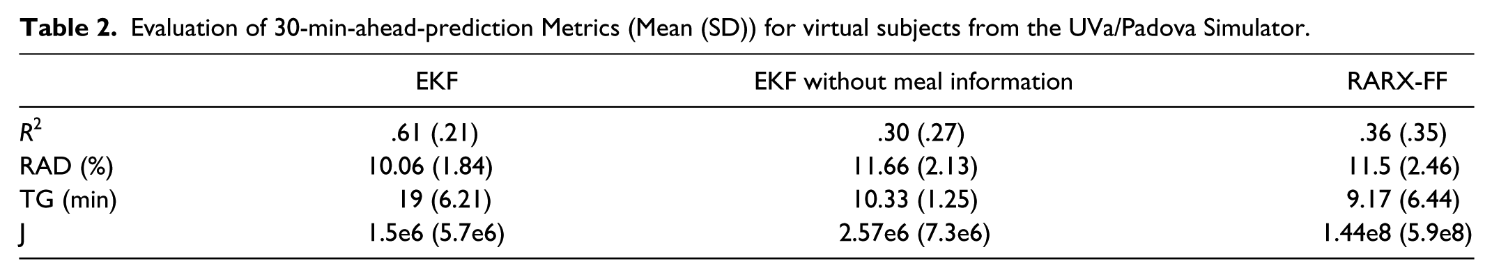
Table 2 lists the mean and standard deviation values of the prediction performance metrics for a 30-minute prediction horizon for the 30 virtual subjects in the UVa/Padova simulator. A 30-minute prediction horizon was chosen based on the fact that meal announcement is often given 30 minutes ahead. Meal information would often not be available for a longer time horizon to compute the future glucose prediction for control design of insulin delivery. Table 2 shows that on average, the EKF model has an 70% increase in R², 10-minute increase in TG, and about 100 times lower value in J, compared to the RARX-FF model. Since the lower bound of 70 mg/dl glucose value was not violated for the virtual subjects, sensitivity and false alarm rate for early detection of hypoglycemia could not be evaluated for these virtual subjects. Nevertheless, it should be noted that the index J should provide an informative measure of the usability of the predicted profile in detection of hypoglycemia.³²

Table 2.

Evaluation of 30-min-ahead-prediction Metrics (Mean (SD)) for virtual subjects from the UVa/Padova Simulator.

	EKF	EKF without meal information	RARX-FF
R ²	.61 (.21)	.30 (.27)	.36 (.35)
RAD (%)	10.06 (1.84)	11.66 (2.13)	11.5 (2.46)
TG (min)	19 (6.21)	10.33 (1.25)	9.17 (6.44)
J	1.5e6 (5.7e6)	2.57e6 (7.3e6)	1.44e8 (5.9e8)

Among the 30 virtual subjects, the prediction by the EKF model has the highest R² value (R² = .86) for adolescent 5 (given by Figure 2a) and lowest R² value (R² = .16) for adolescent 6 (given by Figure 3a). Estimates of time-varying model coefficients of the EKF models are given in Figure 2b for adolescent 5 and in Figure 3b for adolescent 6. Figure 2a shows that the EKF predictions follow more promptly the ascending and descending portions of the glucose than do the RARX-FF predictions, demonstrating that EKF has higher TG than RARX-FF, though the EKF has a slightly higher over-prediction in peak values of glucose. Figure 3a shows that for adolescent 6, misprediction of peak and valley values of the postprandial glucose are fairly severe, which leads to R² = .16 (compared to R² = –.35 for RARX-FF). The low R² value for adolescent 6 is mainly due to the highly variable CGM of the interstitial fluid compared to the ideal interstitial glucose (not shown), that is, large ratio of the sensor measurement error over the interstitial glucose. If the model for adolescent 6 were used for the model-based control for insulin delivery, a smaller prediction horizon would need to be used. Nevertheless, one advantage of using the EKF model prediction lies in that the error covariance of the prediction can be computed, that is, the uncertainty associated with the prediction can be quantified and then used for control design.

Figure 2.

Model prediction for adolescent 5. (a) Glucose predictions by EKF, EKF without meal information, and RARX-FF (where CGM refers to the sensor-measured interstitial glucose output from the UVa/Padova simulator). (b) Estimates of model coefficients of EKF model.

Figure 3.

Model prediction for adolescent 6. (a) Glucose predictions by EKF, EKF without meal information, and RARX-FF (where CGM refers to the sensor-measured interstitial glucose output from the UVa/Padova simulator). (b) Estimates of model coefficients of EKF model.

From Figure 2a and Figure 3a, we can see that meal information plays an important role in model prediction for postprandial glucose. At fasting time or around 3 hours after meal, the predictions from EKF and EKF without meal information are very close; however, right after each meal (t = 7 hours, 12 hours, and 18 hours), the delay associated with the EKF model without meal information is pretty obvious. Table 2 also shows that without meal information, both the model fitness and TG reduce by half compared to the model with meal information.

Clinical Patients

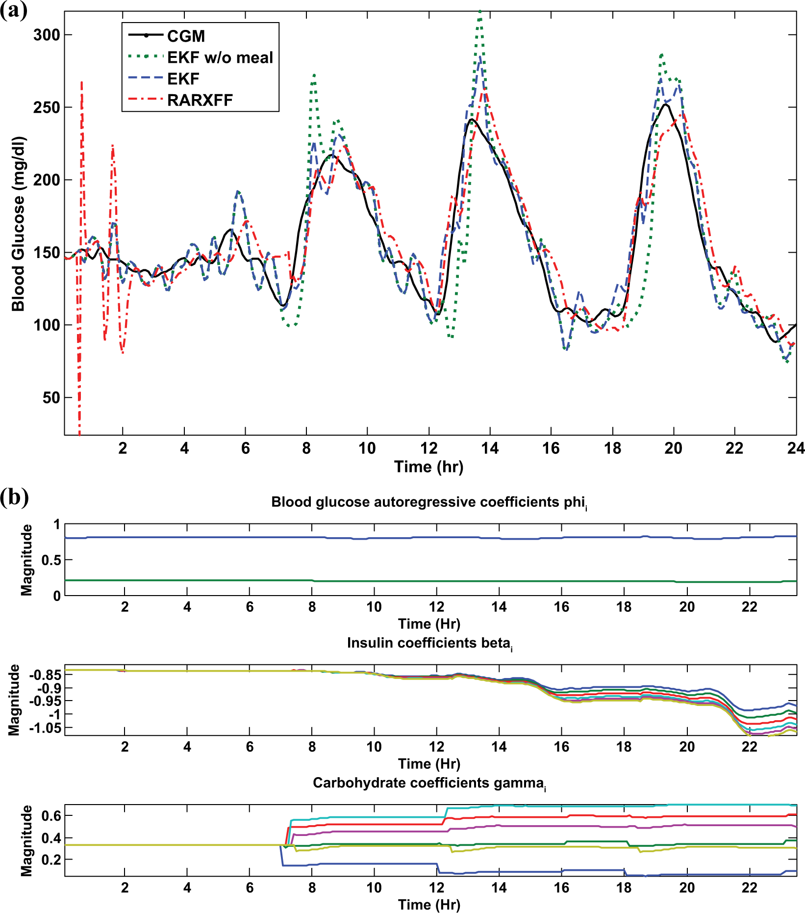
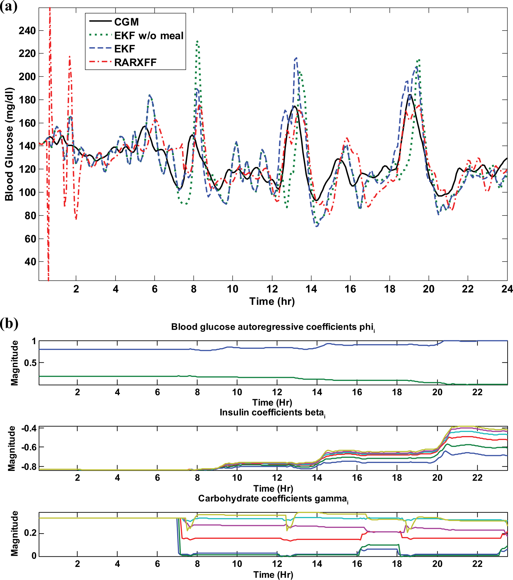
Table 3 lists the mean and standard deviation of the 30-minute-ahead prediction performance metrics for 5 clinical diabetic patients. Model predictions for a representative real subject (patient 4) are shown in Figure 5, and patient 4’s CGM, insulin delivery, and carbohydrate time series are given in Figure 4 for reference. To allow the readers to better view the differences between the predictions and the CGM, we separate patient 4’s time series from day 1 and day 2 in 2 subplots. As can be seen, it takes some significant time for the RARX-FF model to converge (as illustrated by the first day’s CGM and prediction shown in Figure 5). In Table 3, we compute the statistics using predictions starting from the second day for all 5 patients.

Table 3.

Evaluation of 30-min-ahead-prediction Metrics (Mean (SD)) for Clinical Patients Under Free-living Conditions: Statistics Computed Using Predictions Starting From the Second Day for All Patients.

	EKF	EKF without meal information	RARX-FF
R ²	.71 (.19)	.71 (.18)	.64 (.24)
RAD (%)	20.31 (10.44)	20 (9.8)	22.2 (11.83)
TG (min)	12 (10.37)	6 (6.52)	1.00 (2.24)
J	377.93 (644.32)	∞*	∞*
Sensitivity (%)	78.71 (7.26)	79.3 (7.48)	71.43 (15.74)
False alarm rate (%)	35.60 (9.61)	39.14 (10.8)	34.77 (3.26)

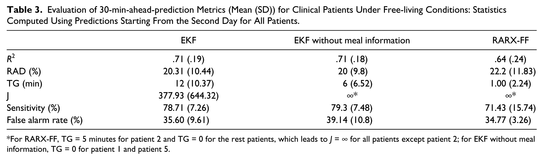
For RARX-FF, TG = 5 minutes for patient 2 and TG = 0 for the rest patients, which leads to J = ∞ for all patients except patient 2; for EKF without meal information, TG = 0 for patient 1 and patient 5.

Figure 4.

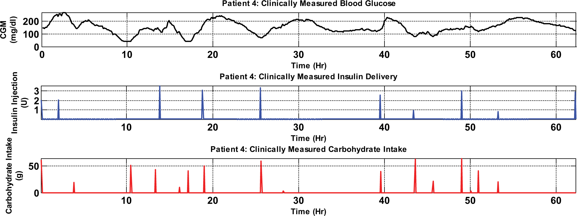
Time series for patient 4: continuous interstitial glucose monitoring, insulin delivery, and carbohydrate intake.

Figure 5.

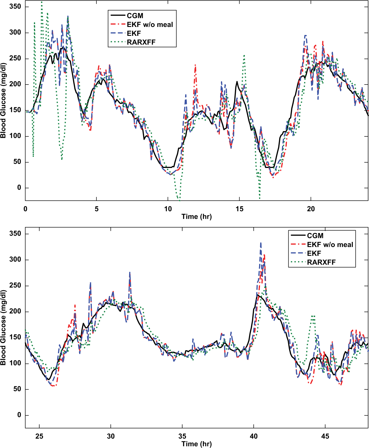
Clinical patient 4: 30-minute-ahead predictions by the EKF, EKF without meal information, and RARXFF. Top: 0-24 hours; bottom: 24-48 hours.

Table 3 shows that, starting on day 2, the EKF predictions demonstrate 10% increase in R² compared to the RARX-FF, but the EKF results have significantly higher TG values (more than 10 minutes temporal gain) than RARX-FF, whose temporal gain is 0 for 4 patients except TG = 5 minutes for patient 2. Figure 4 also shows clearly time delay in predictions by the RARX-FF. For a hypoglycemia alarm threshold of 70 mg/dl, the EKF model was able to predict, on average, 78.7% of the hypoglycemic events with a false alarm rate of 35.6% and 12 minutes (TG) ahead of time. It is well-known that the choice of the hypoglycemia threshold could drastically affect the sensitivity and false alarm rate of the prediction algorithm,^12,20 and thus the J index is used to provide supplementary measure on the usability and reliability of the prediction and hypoglycemia detection. As shown in Table 3, while the RARX-FF has similar sensitivity and false alarm rate as the EKF in terms of the 70 mg/dl hypoglycemia threshold, it does not provide early detection due to its near 0 temporal gain.

Figure 5 also shows that with meal information, even though gross errors in estimating carbohydrate intake for clinical patients are very likely, the EKF prediction for postprandial glucose is still better than the EKF model without meal information. At t = 11 hours, 17 hours, 26 hours, and 43 hours, the delay associated with the EKF model without meal information is pretty obvious. Table 3 shows that though the point-to-point fitness values are very close for EKF models with or without meal information, TG of the model without meal information is only half of that with meal information.

Consistency of the EKF

The filter consistency of the EKF in estimating glucose levels for the virtual subjects and the 5 clinical diabetic patients was evaluated using the single-run normalized innovation squared, and the resulting NIS ψ (t) $ψ (t)$ was found to lie in its 95% probability region [0, 3.4848] of a chi-square distribution. The time-average normalized innovation squared, was also evaluated and found to confirm the consistency of the EKF, for example, $\bar{ψ} = 0.0015 \in [0, 1.14]$ for adolescent 5; $\bar{ψ} = 0.18 \in [0, 1.14]$ for adolescent 6;and $\bar{ψ} = 0.01155 \in [0, 1.097],$ $\bar{ψ} = 0.00195 \in [0, 1.0841],$ $\bar{ψ} = 0.00779 \in [0, 1.097],$ $\bar{ψ} = 0.00200 \in [0, 1.0822]$ , and $\bar{ψ} = 0.00204 \in [0, 1.0805]$ for clinical patients 1 to 5, respectively.

Discussion

In this article we present the application of a new inductive approach to prediction and dynamic regression of continuously monitored glucose on insulin dose and carbohydrate intake and the results are generally encouraging. The parameter estimates in the patient-specific state-space models in this article show considerable time-dependent variation as well as variation between subjects. This holds especially for the beta and gamma coefficients in the dynamic regressions of blood glucose on, respectively, insulin dose and carbohydrate intake, reflecting the complexity of the physiology that is difficult for theoretically based models to describe.

While the sensitivity for detection of hypoglycemia is good (almost 80%, TG in the range of 10-20 minutes), the false alarm rate is relatively high. Note that the sensitivity and false alarm rate are highly dependent on the choice of threshold value. In addition, the false alarm rate is significantly affected by the uncertainty as well as measurement noise associated with the CGM time series. In future work, we plan to consider a band rather than a single threshold value by utilizing the error covariance prediction obtained in the EKF.

Note that though according to the existing literature, pure autoregressive models without inputs such as the AR and ARMA models, and the zero-order-hold model could provide decent glucose prediction in terms of the point-to-point accuracy, they cannot be used for control purposes. The EKF based state-space model developed in this article is particularly suitable for model-based state-feedback control designs since the Kalman filter estimates the state variable (glucose concentration) of the glucose dynamics based on the CGM time series; preliminary results have been obtained on a receding horizon control using the proposed model.³⁷ By estimating model parameters in real time, the EKF model presented here could be combined with the adaptive control technique to design an adaptive controller for insulin delivery.³⁸

We recognize that the veracity of any model that predicts glucose in type 1 diabetic patients depends on the quality of information about insulin dose and food intake. Supplying insulin-dose-delivered information to the model is relatively trivial, but gross errors in providing food information are likely. Thus, as the next step, we will explore model predictions where failure to provide meal information occurs, for example, complete forgetting of meal notification or failure to eat a meal after meal notification. Past research includes adaptive meal detection algorithms,³⁹ and probabilistic description of food intake.^40,41 One possible approach we plan to explore to address the misinformation on food in the modeling is to treat the food intake as an unknown input and to extend our EKF-based modeling framework by including adaptive estimation algorithms,²⁹ which can be applied to estimate the unknown input of a system in real time via state augmentation.

Conclusions

In this article, we have developed an empirical state-space model for glucose dynamics of type 1 diabetes by an EKF. Inputs of insulin delivery and carbohydrate intake in the glucose dynamics are modeled. Compared to a forgetting-factor-based recursive ARX model of the same order and based on evaluation of 30 virtual subjects and 5 clinical patients, the EKF model predictions have higher R² values and significantly better temporal gain and J index, and thus are superior in early detection of upward and downward trends in glucose. We expect our EKF-based modeling approach to be a powerful tool in modeling glucose dynamics in insulin deficient diabetes that can be used for state-feedback control design of optimal dose of insulin delivery.

Footnotes

Appendix A

Appendix B

Appendix C

Acknowledgements

We would like to thank Jing Zhou for the contribution on implementation of part of the modeling algorithms. The services provided by the General Clinical Research Center of Pennsylvania State University are appreciated, as is the study coordination of Joanna Lyons and the study subjects.

Abbreviations

ARX, autoregressive exogenous input; CGM, continuous glucose monitoring; EKF, extended Kalman filter.

Declaration of Conflicting Interests

The author(s) declared no potential conflicts of interest with respect to the research, authorship, and/or publication of this article.

Funding

The author(s) disclosed receipt of the following financial support for the research, authorship, and/or publication of this article: This project was supported in part by NIH Grant M01 RR 10732; NSF Grants 0852147, 1157220, and 1200838; and Penn State CTSI.

References

Hovorka

. The future of continuous glucose monitoring: closed loop. Curr Diabetes Rev. 2008;4(3):269-279.

Parker

Doyle

Peppas

. A model-based algorithm for blood glucose control in type I diabetic patients. IEEE Trans Biomed Eng. 1999;46(2):148-157.

Hovorka

Shojaee-Moradie

Carroll

. Partitioning glucose distribution/transport, disposal, and endogenous production during IVGTT. Am J Physiol. 2002;282(5):992-1007.

Steil

Clarak

Kanderian

Rebrin

. Modeling insulin action for development of a closed-loop artificial pancreas. Diabetes Technol Ther. 2005;7(1):94-108.

Gani

Gribok

Rajaraman

Ward

Reifman

. Predicting subcutaneous glucose concentration in humans: data-driven glucose modeling. IEEE Trans Biomed Eng. 2009;56(2):246-254.

Bequette

. Continuous glucose monitoring: real-time algorithms for calibration, filtering, and alarms. J Diabetes Sci Technol. 2010;4(2):404-418.

Sparacino

Facchinetti

Cobelli

. Smart continuous glucose monitoring sensors: on-line signal processing issues. Sensors. 2010;10:6751-6772.

Ståhl

Johansson

. Diabetes mellitus modeling and short-term prediction based on blood glucose measurements. Math Biosci. 2009;217:101-117.

Finan

Doyle

III Palerm

. Experimental evaluation of a recursive model identification technique for type 1 diabetes. J Diabetes Sci Technol. 2009;3(5):1192-1202.

10.

Eren-Oruklu

Cinar

Rollins

Quinn

. Adaptive system identification for estimating future glucose concentrations and hypoglycemia alarms. Automatica. 2012;48:1892-1897.

11.

Naumova

Pereverzyev

Sivananthan

. A meta-learning approach to the regularized learning—case study: blood glucose prediction. Neural Netw. 2012;33:181-193.

12.

Zecchin

Facchinetti

Sparacino

De Nicolao

Cobelli

. Neural network incorporating meal information improves accuracy of short-time prediction of glucose concentration. IEEE Trans Biomed Eng. 2012;59(6):1550-1560.

13.

Hovorka

. Management of diabetes using adaptive control. Int J Adaptive Control Signal Processing. 2005;19:309-325.

14.

Eren-Oruklu

Cinar

Quinn

Smith

. Estimation of future glucose concentrations with subject-specific recursive linear models. Diabetes Technol Ther. 2009;11(4):243-253.

15.

Sparacino

Zanderigo

Corazza

Maran

Facchinetti

Cobelli

. Glucose concentration can be predicted ahead in time from continuous glucose monitoring sensor time-series. IEEE Trans Biomed Eng. 2007;54(5):931-937.

16.

Reifman

Rajaraman

Gribok

Ward

. Predictive monitoring for improved management of glucose levels. J Diabetes Sci Technol. 2007;1(4):478-486.

17.

EI-Khatib

Jiang

Damiano

. Adaptive closed-loop control provides blood-glucose regulation using dual subcutaneous insulin and glucagon infusion in diabetic swine. IEEE Trans Biomed Eng. 2007;54(5):931-937.

18.

Perez-Gandia

Facchinetti

Sparacino

. Artificial neural network algorithm for online glucose prediction from continuous glucose monitoring. Diabetes Technol Ther. 2010;12(1):81-88.

19.

Pappada

Cameron

Rosman

. Neural network-based real-time prediction of glucose in patients with insulin-dependent diabetes. Diabetes Technol Ther. 2011;13(2):135-141.

20.

Palerm

Bequette

. Hypoglycemia detection and prediction using continuous glucose monitoring—a study on hypoglycemic clamp data. J Diabetes Sci Technol. 2007;1(5):624-629.

21.

Palerm

Willis

Desemone

Bequette

. Hypoglycemia prediction and detection using optimal estimation. Diabetes Technol Ther. 2005;7(1):3-14.

22.

Facchinetti

Sparacino

Cobelli

. An online self-tunable method to denoise CGM sensor data. IEEE Trans Biomed Eng. 2010;57(3):634-641.

23.

Facchinetti

Sparacino

Cobelli

. Enhanced accuracy of continuous glucose monitoring by online extended Kalman filtering. Diabetes Technol Ther. 2010;12(5):353-363.

24.

Knobbe

Buckingham

. The extended Kalman filter for continuous glucose monitoring. Diabetes Technol Ther. 2005;7:15-27.

25.

Dalla Man

Camilleri

Cobelli

. A system model of oral glucose absorption: validation on gold standard data. IEEE Trans Biomed Eng. 2006;53(12):2472-2478.

26.

Lehman

Deutsch

. A physiological model of glucose-insulin interaction in type 1 diabetes mellitus. J Biomed Eng. 1992;14:235-242.

27.

Elashoff

Reedy

Meyer

. Analysis of gastric emptying data. Gastroenterology. 1982;83:1306-12.

28.

Dalla Man

Rizza

Cobelli

. Meal simulation model of the glucose-insulin system. IEEE Trans Biomed Eng. 2007;54(10):1740-1749.

29.

Bar-Shalom

Kirubarajan

. Estimation with Applications to Tracking and Navigation. New York, NY: John Wiley; 2001.

30.

Young

. Nonlinear and Nonstationary Signal Processing. Chapter: Stochastic, Dynamic Modeling and Signal Processing: Time Variable and State Dependent Parameter Estimation. Cambridge, UK: Cambridge University Press; 2000.

31.

Finan

Palerm

Doyle

III . Effect of input excitation on the quality of empirical dynamic models for type 1 diabetes. Process Syst Eng. 2009;55(5):1135-1146.

32.

Facchinetti

Sparacino

Trifoglio

Cobelli

. A new index to optimally design and compare CGM glucose prediction algorithms. Diabetes Technol Ther. 2011;13(2):111-119.

33.

Kovatchev

Breton

Dalla Man

Cobelli

. In silico preclinical trials: a proof of concept in closed-loop control of type 1 diabetes. J Diabetes Sci Technol. 2009;3(1):44-55.

34.

Berger

Rodbard

. Computer-simulation of plasma-insulin and glucose dynamics after subcutaneous insulin injection. Diabetes Care. 1989;12:725-736.

35.

Hovorka

. Continuous glucose monitoring and closed-loop systems. Diabetes Med. 2006;23(1):1-12.

36.

Goodwin

Sin

. Adaptive Filtering, Prediction and Control. Englewood Cliffs, NJ: Prentice Hall; 1984.

37.

Zhou

Wang

Molenaar

Ulbrecht

Gold

Rovine

. Receding horizon control of type 1 diabetes based on a data-driven linear time-varying state-space model. Paper presented at: American Control Conference; 2010; Baltimore, MD.

38.

Freeman

Wang

Molennar

Ulbrecht

Gold

Rovine

. Development of an adaptive dual controller for glucose management in patients with insulin-deficient diabetes. Paper presented at: ASME Dynamic Systems and Control Conference; October 2012; Fort Lauderdale, FL.

39.

Patek

Breton

Dalla Man

Cobelli

Kovatchev

. Adaptive meal detection algorithm for enhancing closed-loop control in type 1 diabetes. Paper presented at: Diabetes Technology Meeting; 2007; San Francisco, CA.

40.

Patek

Hughes

Breton

Kovatchev

. Anticipating meals with behavioral profiles: towards stochastic model predictive control of t1dm. Paper presented at: 7th IFAC Symposium on Biological and Medical Systems; August 2009; Aalborg, Denmark.

41.

Cameron

Bequette

Buckingham

Wilson

Lee

Niemeyer

. Anticipatory behavior in blood glucose control: using meal prior probabilities to prepare for future meal disturbances. Paper presented at: IFAC World Congress, August 28-September 2, 2011; Milano, Italy.

Personalized State-space Modeling of Glucose Dynamics for Type 1 Diabetes Using Continuously Monitored Glucose,Insulin Dose,and Meal Intake

Abstract

Background:

Methods:

Conclusion:

Keywords

Methods

Time-varying State-space Model for Glucose Dynamics

FIR Modeling of Subcutaneous Insulin Absorption and Meal Absorption

Extended Kalman Filter to Estimate the Time-varying Coefficients and Glucose Level Simultaneously

Consistency of the Extended Kalman Filter

Model Evaluation Metrics

Data Base

FDA-approved UVa/Padova T1DM Simulator and Virtual Subjects

Free-living Type 1 Diabetic Patient Data

Results

Model Parameters

Simulation Results

Virtual Subjects from the UVa/Padova Simulator

Clinical Patients

Consistency of the EKF

Discussion

Conclusions

Footnotes

Appendix A

Appendix B

Appendix C

Acknowledgements

Abbreviations

Declaration of Conflicting Interests

Funding

References