Sage Journals: Discover world-class research

Abstract

Background

Freezing of gait (FoG) is a complex, frequent, and disabling motor symptom of Parkinson’s disease (PD). Wearable technology has the potential to improve FoG assessment by providing objective, quantitative, and continuous monitoring.

Objective

This study aims to develop a robust FoG detection algorithm that can be embedded in a simple and unobtrusive wearable sensor system and can lead to a reliable unsupervised home assessment.

Methods

Twenty-two subjects with PD and FoG were enrolled, equipped with four inertial modules on the ankles, back, and wrist, and asked to perform different tasks. Feature-driven and data-driven machine learning approaches were implemented, optimized, and evaluated. Further testing was conducted on two external datasets including a total of 545 FoG episodes.

Results

Sixteen subjects experienced FoG, providing a total number of 101 FoG events. Results demonstrated that a single sensor on the ankle, with an adequate algorithm of data analysis based on machine learning, can provide a non-invasive approach for accurate FoG detection. The model proved robust on the independent datasets, with 88–95% FoG episodes correctly detected. Interestingly, while FoG can be easily discriminated from walking, static positions, and postural transitions, turning represents a significant challenge. The high number of false alarms still represents the main limitation of the FoG recognition algorithms.

Conclusions

The collected dataset includes data from different sensors at different body positions. This, together with detailed labeling of tasks, activities, FoG episodes and their severity, can be a significant contribution to research on automatic FoG detection and characterization.

Keywords

Parkinson’s disease freezing of gait wearable sensor machine learning deep learning detection

Introduction

Parkinson’s disease (PD) is the second most common neurodegenerative disease, with over 10 million people affected in the world.^1,2 One of the most disabling PD symptoms is freezing of gait (FoG), which is a relevant cause of gait impairment, instability, and falls. Management of FoG is an unmet need. It is often poorly recognized because of its episodic nature, the variability of triggering situations, and the reporting bias of patients and caregivers.^3,4 Difficulties in reliable assessment and monitoring of FoG have hampered the research on the intricate pathophysiology of FoG, particularly its management. Pharmacological treatments for FoG are limited to those associated with off and wearing-off states.^3,5 Administration of cues with different sensory modalities (e.g., auditory, visual, proprioceptive) can be used to prevent/reduce FoG episodes.⁶ However, continuous external cueing may compromise efficacy, while personalized on-demand cueing (i.e., stimulation upon FoG detection) has proved effective in reducing FoG duration in both supervised laboratory experiments and unsupervised daily life.⁷ The current standard for FoG assessment, both in clinical and research settings, is based on validated questionnaires, which are limited by recall bias and can only capture in general the severity of FoG episodes during an extended period of time.^8,9 Moreover, FoG questionnaires are considered not adequate as an outcome measure for clinical trials due to their low accuracy in detecting changes in FoG frequency and severity.^10,11

In this context, wearable inertial sensors have been employed in research settings to detect the presence of FoG episodes.^12–14 Although wearable devices hold promise for low-cost data acquisition, the information they generate requires processing to extract clinically meaningful information. Consequently, the large volume of data can be effectively managed by applying artificial intelligence and data analysis methodologies. In particular, machine learning (ML) has emerged as a key component in the creation of remote monitoring systems based on wearable devices. ML algorithms offer the ability to examine sensor data, enabling the extraction of valuable insights or the revelation of hidden patterns in a semi-automated manner.¹⁵ Feature-driven ML relies on the extraction and selection of relevant features from the input data.¹⁶ These features are carefully crafted and chosen based on domain knowledge and understanding of the problem at hand. In essence, the success of feature-driven approaches heavily relies on the expertise of human practitioners in identifying the most informative aspects of the data,^17,18 although many libraries exist that can automate feature extraction and selection processes on time series data (e.g., tsfresh¹⁹ or tsflex²⁰). In contrast, data-driven deep learning (DL) harnesses the power of artificial neural networks to automatically learn hierarchical representations directly from the raw data. In this paradigm, the model autonomously discovers intricate patterns and features during the training process.²¹ DL methods, such as convolutional neural networks (CNNs), recurrent (e.g., long short-term memory – LSTM, gated recurrent units –GRU) and Transformer neural networks, are particularly suitable for capturing complex relationships within large datasets.²²

Recent advances in ML and DL have provided promising results in automatic FoG recognition from wearable sensors data.^22–28 Furthermore, recent studies have explored the importance of sensor placement, task-related factors, patient preferences, and user acceptance in both laboratory and unsupervised real-world applications to advance the detection and management of FoG.^26–30 Despite these advances, there is a significant lack of consensus on the best procedures for FoG detection, including variations in the number and types of sensors used for data collection.²² In addition, there is evidence of a paucity of publicly available datasets containing FoG data. At present, only five public datasets exist.^{26,29,31–33} Some of these datasets include only accelerometer recordings, devoid of contextual information regarding activity during FoG events.³⁴ However, there is evidence that artificial intelligence algorithms may fail to generalize to new tasks and activities.²⁷ In this context, information on contextual activities (e.g., walking, turning, stopping) can provide valuable insights into FoG detection errors and help to better design training strategies. Moreover, few studies have comprehensively evaluated the performance of FoG detection algorithms on external and independent datasets.²² This gap is critical to realistically evaluate the performance and generalization ability of these algorithms.^35,36

The present study aims to collect a dataset with accelerometers and gyroscopes strategically placed at various locations on the body. Careful identification of the beginning and end of each FoG episode is ensured, and common activities are meticulously labeled to establish a contextual background for FoG manifestations. Feature-driven and data-driven ML approaches are implemented and optimized, and the effect of sensor location, sensor type, and different activities is evaluated. The effectiveness of the algorithms on external datasets is evaluated to assess their generalization ability. Finally, a comprehensive evaluation of FoG detection is conducted, including the analysis of false positives and the calculation of prediction time and detection delay for possible closed-loop automatic application of cues to help subjects with PD to overcome FoG.

Materials and methods

Study design and participants

Twenty-two patients affected by idiopathic PD according to the international Movement Disorder Society diagnostic criteria, were enrolled in this study from two university movement disorders clinics (University Hospital Trust of Torino, Department of Neurosciences and Mental Health, Turin, Italy; University Hospital Trust of Verona, Department of Neurosciences, Biomedicine and Movement Sciences, Verona, Italy). Inclusion criteria were: (a) diagnosis of idiopathic PD,³⁷ (b) H&Y score between 2 and 4, (c) daily FoG episodes reported in the last month according with a score of 1 on Question 1 and score $\geq$ 2 on Question 2 of the New Freezing of Gait Questionnaire,³⁸ (d) to be under stable PD treatment for more than one month, (e) to be able to walk continuously and independently (the use of walking aids like a cane or a rollator was permitted) for at least fifteen minutes, and (f) no dementia, relevant musculoskeletal, cardiovascular, psychiatric or other neurological conditions that may have significantly affected the gait. Participants were asked not to take their last medication since the day before experiments, and so evaluated in the morning in the so-called OFF therapeutic condition (> 12 h since the last intake of dopaminergic drugs, avoiding prolonged release pills intake and/or removing patches the night before the experiment when applicable). All clinical evaluations have been conducted in the morning, and followed by the data acquisition process.

All participants provided written informed consent prior to their inclusion. The study received approval from the institutional review boards and has been performed in accordance with the Declaration of Helsinki. The study received approval from the ethics committee for clinical trials of the provinces of Verona and Rovigo (approval n^o 3670CESC), Italy and Città della Salute e della Scienza di Torino (approval n $^{o}$ 0086153), Italy.

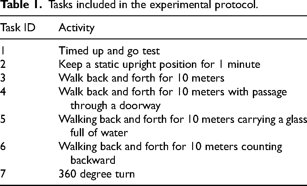
Participants were asked to perform different tasks, with a self-selected rest between them. They were instructed on how to perform the task before data collection started. Moreover, they were free to quit the experiments whenever they wanted. Table 1 reports the tasks performed in this study. Task 1 consisted of the timed-up-and-go test, which requires the user to stand up from a chair, walk back and forth for 10 meters, and sit in the same chair. In task 2, the subject was asked to keep a static upright position for one minute. Tasks 3 to 6 consist of a 10-meter walking back and forth task with or without dual-task and/or obstacles. Specifically, task 3 represents the standard walking task. Task 4 included a passage through a doorway. In task 5, a motor dual task was included, which required patients to carry a glass full of water in their hand. Task 6 included a cognitive dual-task, in which subjects were asked to count backward from 100 to 0 while walking. Finally, task 7 involved 360-degree turns in both directions.

Table 1.

Tasks included in the experimental protocol.

Task ID	Activity
1	Timed up and go test
2	Keep a static upright position for 1 minute
3	Walk back and forth for 10 meters
4	Walk back and forth for 10 meters with passage through a doorway
5	Walking back and forth for 10 meters carrying a glass full of water
6	Walking back and forth for 10 meters counting backward
7	360 degree turn

Instrumentation

Participants were equipped with four inertial measurement units (IMU). Each IMU (Nordic Thingy 52 - NRF6936, Nordic Semiconductor) is a compact device measuring 6 $\times$ 6 cm and weighing 47 grams. The IMU integrates a 9-axis motion-sensing module, which includes a 3-axis accelerometer, gyroscope and compass. It also has a Bluetooth low-energy interface for data transmission and a power supply. In addition to motion sensors, the device includes a microphone and speaker, and humidity, temperature, pressure, gas, color and light sensors. However, only the accelerometer and gyroscope sensors were used in this study. The accelerometer presents a settable full-scale ranging from $\pm 2$ g to $\pm 16$ g and a sensitivity of 4800 LSB/g, while the gyroscope presents a settable full-scale in the range $\pm 250$ dps to $\pm 2000$ dps. In this study, IMUs were configured with the following settings: the full-scale was set to $\pm$ 8 g for the accelerometer and $\pm$ 2000 dps for the gyroscope; data from both sensors were recorded with a sampling rate of 60 Hz. These settings were chosen to ensure accurate and reliable data collection for our application. The data collection was performed using the wireless body area network (WBAN) presented in Demrozi et al.³⁹ and Turetta et al.⁴⁰ The WBAN utilizes an Android smartphone, which has the capability to connect simultaneously to between one and twelve standalone nodes. Additionally, the smartphone can record video through its integrated camera, with the video being synchronized with the nodes’ data streams.

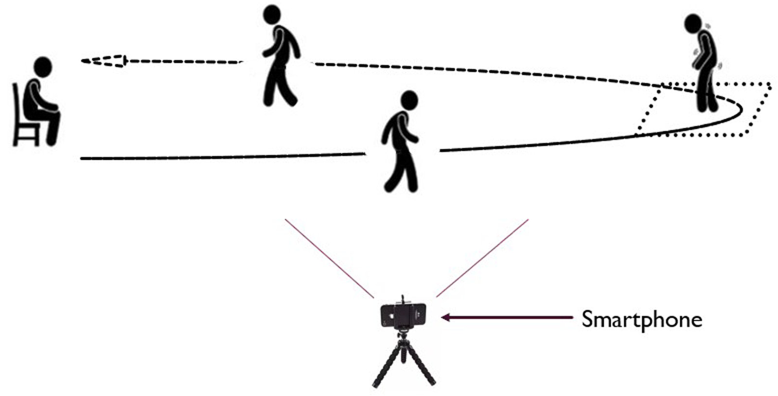
The recorded data from each IMU were sent to a smartphone (Realme Pro 7), which served as a gateway for data collection. An application running on the smartphone facilitated the data collection process. Furthermore, the same smartphone application was utilized for simultaneous video recording at a sampling rate of 30 frames per second (fps) (Figure 1). The smartphone was placed in a specific, predefined location to ensure consistent data collection across all participants. This location was chosen to maximize the visibility and capture of all FoG episodes. The recorded videos were visually inspected in the subsequent data annotation process, providing visual context to the sensor data. The placement of the IMUs on the body is shown in Figure 2. Two sensors were positioned on the outer part of the lower legs, just above the ankles, while another sensor was placed on the lower back at the level of L3-L5 vertebrae.

Figure 1.

Data recording settings.

Figure 2.

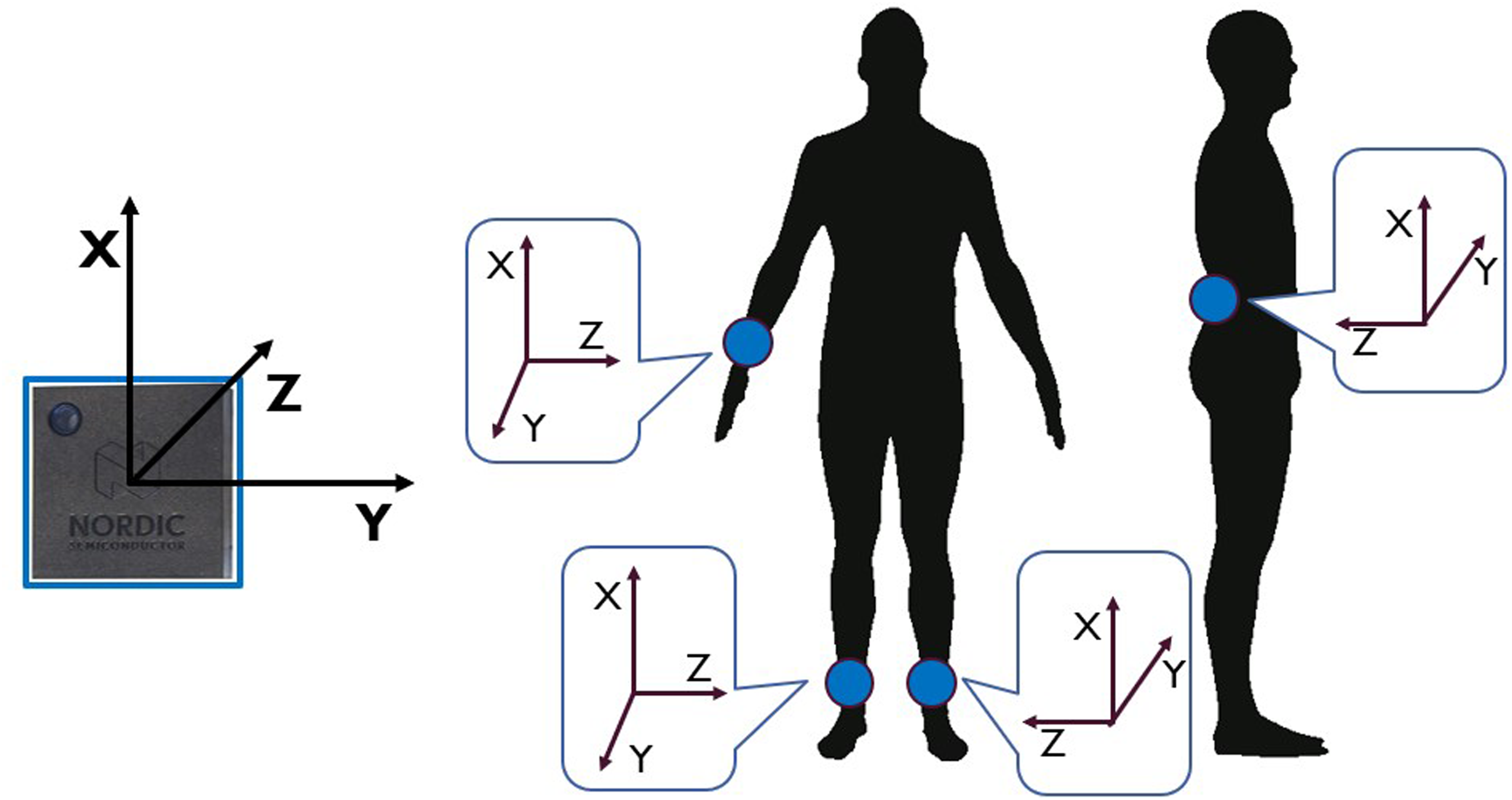
Sensor position and orientation.

The remaining sensor was positioned on the wrist of the most affected side. This sensor setup allowed for capturing detailed motion data from specific body parts and synchronize it with video footage, enhancing the accuracy and context of the collected sensor data for further analysis. To assess participants’ satisfaction with the system, the Quebec user evaluation of satisfaction with assistive technology (QUEST) questionnaire was administered to participants.⁴¹ Specifically, a score between zero and five was assigned to each item concerning the device, namely comfort, weight, durability, adjustments, simplicity of use, dimensions, effectiveness, and safety.

Clinical rating of FoG

Two neurologists (CAA, RAB) experts in PD and movement disorders independently annotated activities and FoG episodes based on an accurate visual inspection of video recordings, according to a predefined, standardized assessment protocol. The definition of FoG (i.e., inability to produce effective steps) and types of FoG (i.e., start hesitation, turn hesitation, FoG during turning, hesitation in tight quarters, destination-hesitation or open space hesitation) were selected according to the literature.^42,43 The evaluators identified the exact start of the FoG episode as the frame corresponding to the end of the last effective step preceding FoG; the end of the FoG episode was identified as the frame corresponding to the first effective step after FoG. The severity of FoG episodes was assigned with a score from 1 to 3, according to the following evaluation: 1: shuffling forward with small steps, 2: trembling in place with alternating rapid knee movements, 3: complete akinesia without limbs or trunk movement. If multiple manifestations were observed within the same FoG episode, the severity score was assigned based on the most severe manifestation.⁴⁴

Video recordings were resampled to 10 fps to ease the annotation process and save time, by using a reduced number of frames. It is worth noting that the sampling frequency was selected to ensure a time resolution of 100 ms in activity and FoG identification. The Python video–annotator software⁴⁵ was used for annotating activities, FoG episodes, and FoG severity for each episode. The resulting labeled data were exported in CSV format and subsequently analyzed. In case of discrepancies in the identification of start, end, or duration of FoG episodes, the two raters were asked to meet and solve inconsistencies, providing a final unique label for that specific episode. Specifically, the discrepancy was identified in the following cases: (a) one rater marked a FoG episode while the other did not (b) there was less than 80% overlap between the episodes identified by the two raters, or (c) a difference of more than 0.5 s in the FoG onset was identified between the two raters. In the remaining cases (i.e., episodes with high inter-rater agreement), the final FoG label in terms of FoG onset and end was calculated as the average of the indications (onset, end) of the two raters. The inter-rater agreement was calculated using the following metrics: (a) intra-class correlation coefficient (ICC) calculated on the number of episodes manifested by each subject; (b) ICC on the percent time spent with FoG (%TF) computed from each subject. In addition, agreement at recording level was detailed for each of the discrepancies.

Data processing

Two approaches were implemented for FoG detection, consisting in a feature-driven ML processing pipeline and a more advanced data-driven DL algorithm. The two methods differ for the pre-processing procedures and the classification model. In the former case, feature extraction, feature selection, and data augmentation are carried to prepare data for input to the ML model. In the latter case, the DL algorithm automatically extracts and selects the most significant features, and performs classification in an end-to-end fashion. For both approaches, data were pre-processed as in Figure 3.

Figure 3.

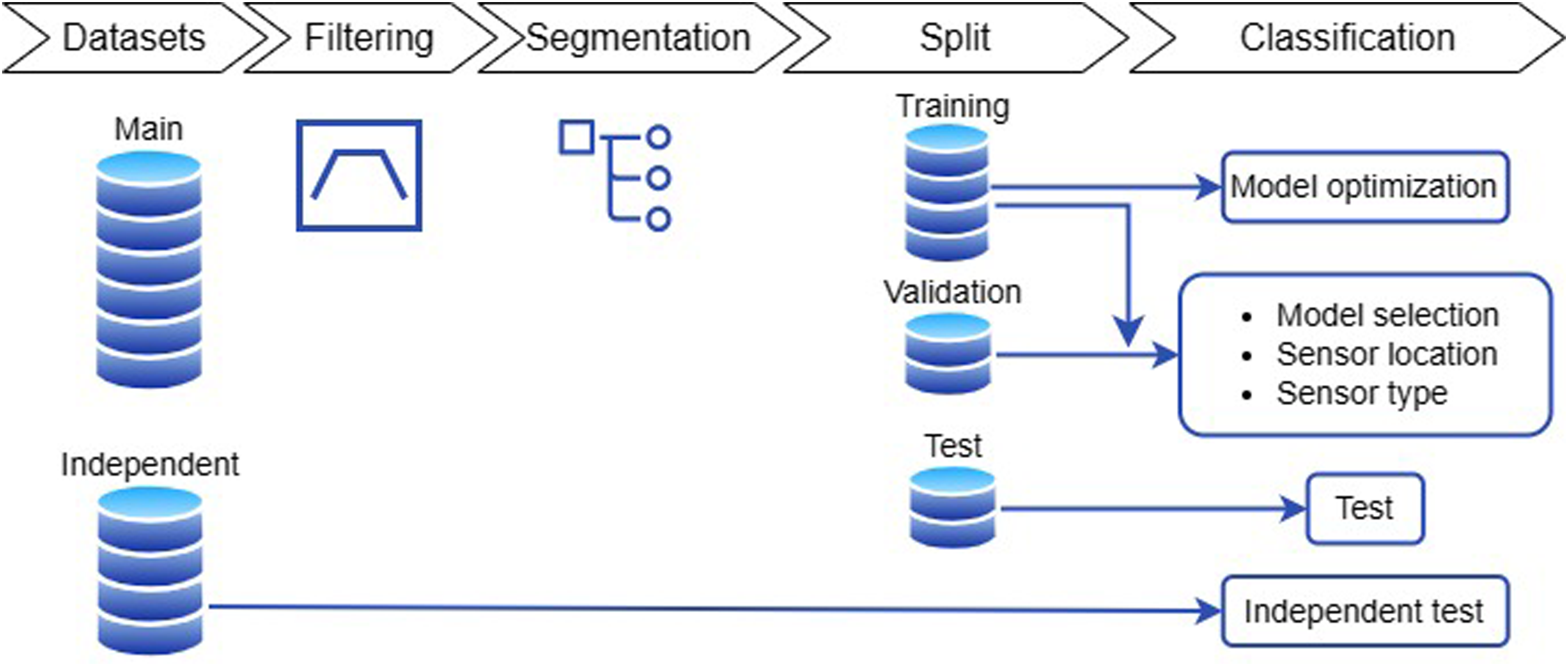
Schematic of the data processing steps.

Data were filtered using a forth-order zero-lag Butterworth band-pass filter with cut-off frequencies of 0.5 Hz and 20 Hz. This allows for removal of gravity and low-frequency trends, and discards high frequency noise. The filtered data were segmented using 2 s-long windows with 75% overlap (0.5 s slide), resulting in a total of 11,280 sliding windows (observations). The window length was selected following previous studies,^35,46 while the large overlap (small slide) has the advantage of providing high temporal resolution in FoG recognition. In addition, isolated windows, i.e., windows classified as FoG/non-FoG while adjacent windows were classified as non-FoG/FoG can be safely discarded (i.e., by using moving mean or majority voting). This is better explained in Figure 4, where a FoG window completely overlaps (grey area) with two adjacent non-FoG windows. This is likely to represent a false positive.

Figure 4.

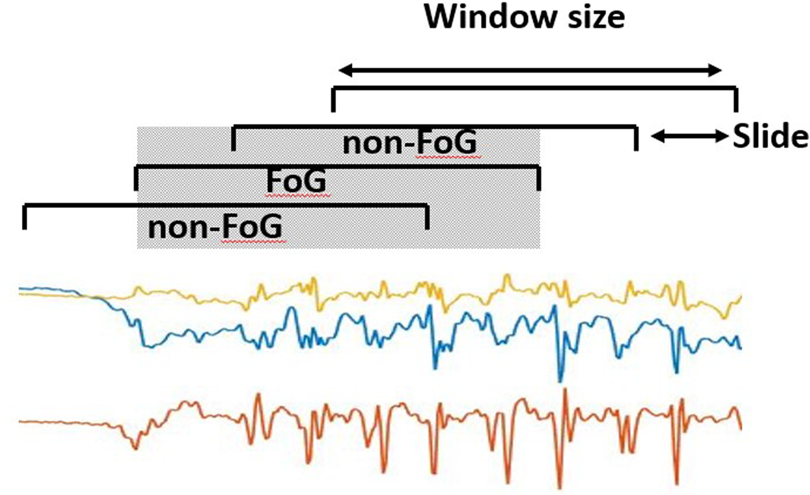
Data segmentation process, consisting in dividing the original signal into 2 s-long windows sliding with 0.5 s advance.

The mean value was removed from each component of each window separately. The generated dataset was split into a training, validation, and test sets, with a proportion of 0.5 (11 subjects), 0.25 (5 subjects) and 0.25 (6 subjects), respectively. Additionally, each subset included at least one non-freezer participant (e.g., 4 in training, 1 in validation and 1 in test). The division was performed by matching subjects in the three sets by age, H&Y, total MDS-UPDRS part-III score, and FoG Questionnaire. Models were trained and optimized on the training set, while performance was evaluated on the validation set. Specifically, the selection of the classification model and its parameters, the sensor location, and sensor type was based on the validation set (Figure 3). The best configuration (i.e., that providing the best performance) was saved and used for testing on the test set, which included new subjects who were not previously assessed. Finally, the model was further tested on two external datasets that included data collected from different subjects in different conditions. This allows us to assess possible over-fitting and obtain a real estimate of the model performance and generalization capability.

Feature-driven approach

Figure 5 schematically reports the feature-driven processing pipeline. A set of features was extracted from the segmented data.

Figure 5.

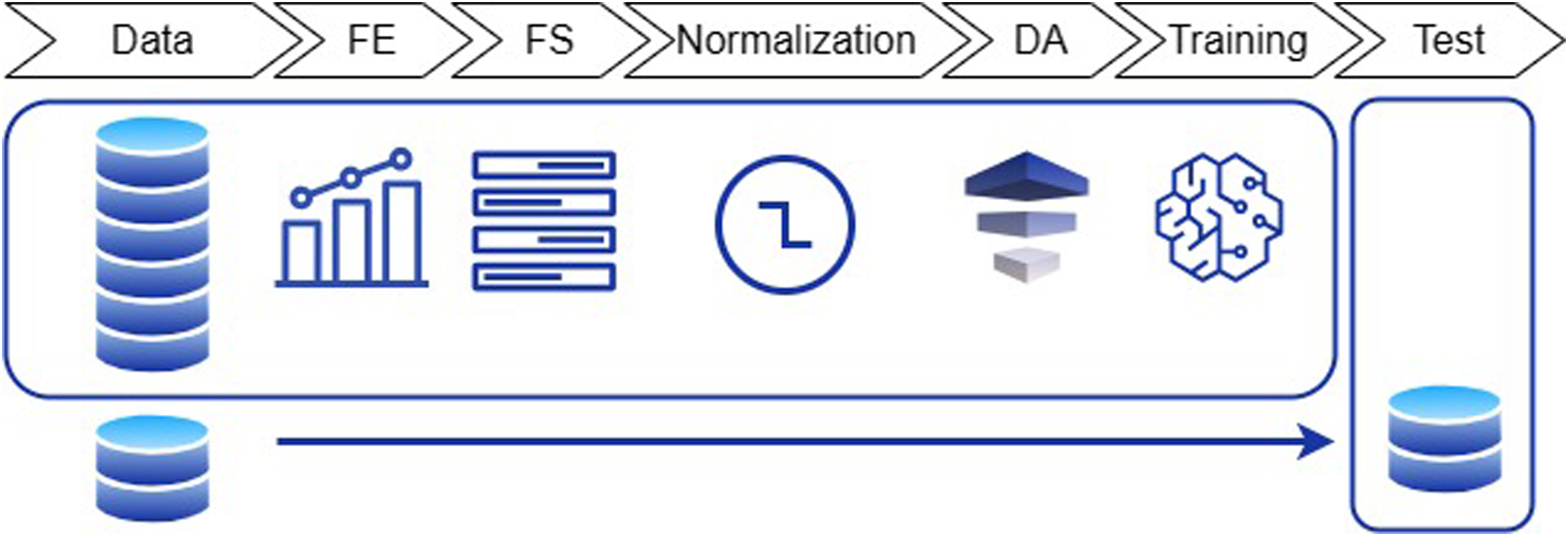
Overview of the feature-driven processing pipeline. FE: feature extraction; FS: feature selection; DA: data augmentation.

All the pre-processing steps described below were based on the training set and applied to the other sets, thus ensuring independent sets. This is particularly important, as the feature selection, normalization, and data augmentation can generate biased results if carried on the entire dataset prior to the training-test split. Each individual processing step is described in the following.

Feature extraction. Table 2 reports the list of temporal and spectral features extracted in this study. Features were extracted from each sensor separately, and from all acceleration and angular velocity components.

Table 2.

List of extracted features. Features were extracted from each component (x,y,z) of each sensor (accelerometer, gyroscope) at each body position (ankles, back, wrist).

ID	Name	Description
1	Mean	Average value
2	Median	Median value
3	STD	Standard deviation
4	RMS	Root mean square value
5	Range	Range of values
6	Min	Minimum value
7	Max	Maximum value
8	Quantile1	25 $^{t h}$ percentile
9	Quantile2	75 $^{t h}$ percentile
10	Entropy	Shannon entropy
11	AAVD	Average absolute value of the first derivative
12	PCA	Principal components analysis coefficients
13	Intensity	Sum of the absolute values of the first derivative
14	Energy	Sum of the absolute value of the signal
15	Corr	Correlation between accelerometer components and gyroscope components
16	Loco-power	Sum of the FFT in the frequency band 0.5–3 Hz
17	Freeze-power	Sum of the FFT in the frequency band 3–8 Hz
18	Freeze-index	Ratio of Freeze-power to Loco-power
19	Freeze-ratio	Percentage of power in the 3–8 Hz band
20	sPeak	Value of the maximum FFT peak
21	sEntropy	Spectral Shannon entropy
22	fEntropy	Spectral Shannon entropy in the 0.5–3 Hz band
23	sKurtosis	Spectral kurtosis
24	fKurtosis	Spectral kurtosis in the 0.5–3 Hz band
25	sSkewness	Spectral skewness
26	fSkewness	Spectral skewness in the 0.5–3 Hz band
27	nPeaks	Number of spectral peaks
28	fHarmonic	Dominant frequency
29	wHarmonic	Width of the principal harmonic
30	aHarmonic	Area of the principal harmonic
31	pHarmonic	Ratio of the height of the principal harmonic and the average harmonics height

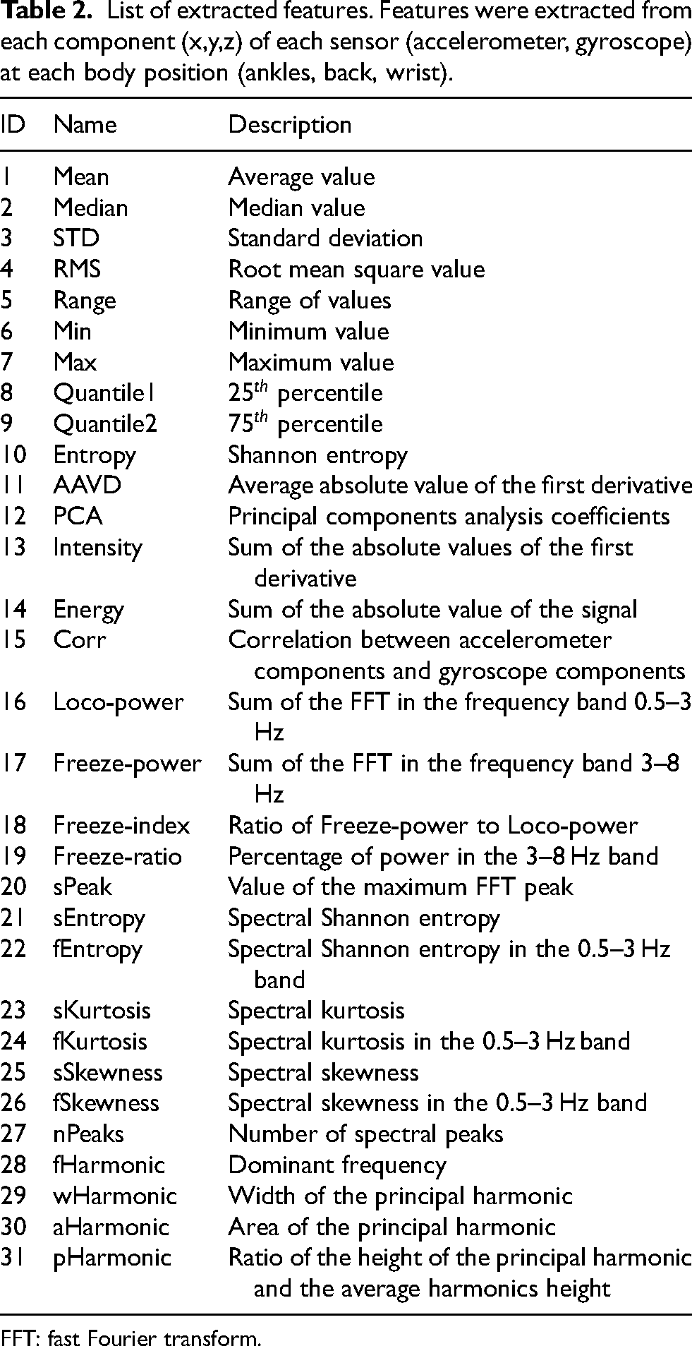
FFT: fast Fourier transform.

For each sensor, a total number of 15 time-domain features were extracted from the preprocessed signals and 16 frequency-domain features were calculated from the fast Fourier transform (FFT). Features were extracted from each signal component ( $α_{x}, α_{y}, α_{z}, ω_{x}, ω_{y}, ω_{z}$ ), providing a total of 186 features. The additional 30 features derive from the principal component analysis coefficients (36 in total).

Feature selection. Features were selected using the minimum redundancy – maximum relevance (mRMR) algorithm.⁴⁷ The algorithm works by selecting the relevant features while controlling for the redundancy within the selected features and is known to be effective in several classification tasks. Based on the training set only, features were ranked in order of importance, and the first $N_{f}$ were selected for the classification task.

Normalization. Feature scaling was performed to uniform the different range of features. Range normalization was employed, defined as in equation (1)

f^{'} = \frac{f - f_{m i n}^{t}}{f_{m a x}^{t} - f_{m i n}^{t}}

(1)

where

f

is the original feature,

f_{m i n}^{t}

and

f_{m a x}^{t}

the minimum and maximum values from the training set, and

f^{'}

the normalized feature.

Data augmentation. The number of FoG samples is smaller than that of the other activities (e.g., walk, turn, static postures), generating an unbalanced class distribution. The synthetic minority oversampling technique algorithm⁴⁸ was used for class balancing. It works by over-sampling the minority class by generating artificial samples obtained as a combination of the original real samples. The over-sampling ratio was obtained as the rounded value of $r = \frac{M^{t}}{m^{t}}$ , where $M^{t}$ and $m^{t}$ correspond to the number of instances in the most (non-FoG) and least (FoG) represented class in the training set, respectively. This ensures optimal class balancing in the training set while keeping the validation/test data unchanged. Moreover, this prevents bias in the results and allows for accurate comparison between feature-driven and data-driven approaches.

Training and classification. A random forest algorithm was used for classification. It represents a well-known and widely used algorithm that has provided top performance in FoG detection.^12,24 The Gini impurity index was set as split criterion. Other model parameters such as the number of estimators (i.e., decision trees), maximum depth, maximum number of splits, and minimum leaf size were optimized, as well as the number $N_{f}$ of selected features. The hyper-parameter optimization procedure was carried using a grid-search approach on a stratified 40% of the training (evaluation set), fine-tuning model hyper-parameters, and selecting those providing the best performance on the evaluation set.

Data-driven approach

The segmented data were input to a CNN. This was selected as data-driven model due to its capability of learning high-level features from large data sets while simplifying the training process and speeding up the computation during inference.^22,49

The implemented model architecture is schematically represented in Figure 6. The CNN has two consecutive convolutional layers followed by a max-pooling layer. A third convolutional block is followed by a max-pooling layer, while the last convolutional layer is connected to a global average pooling layer. The latter is fully-connected to a dense layer, followed by the single output neuron.

Figure 6.

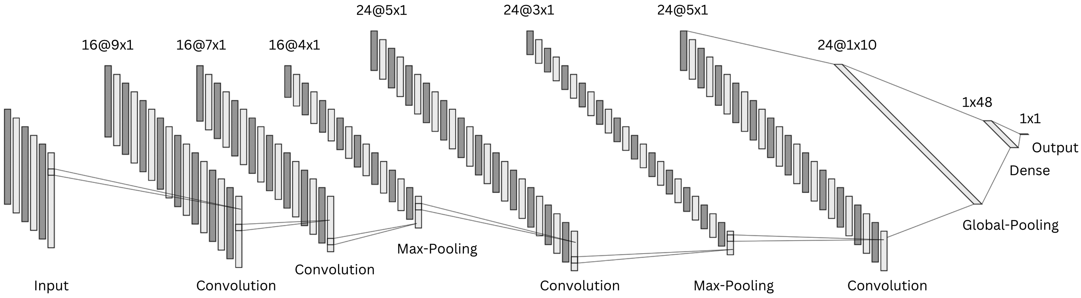
Schematic representation of the implemented one-dimensional convolutional neural network architecture.

Rectified linear unit activation function was used in all layers except for the output, where a sigmoid activation function determines the class probability. Dropout rate of 0.4 and L2 regularization of 0.001 were used in all layers to prevent over-fitting.

The model was trained using a batch size of 64, maximum number of iterations of 120, binary cross-entropy loss-function, and area under the receiver operating characteristic (AUROC) curve metric. Model weights were optimized with the adaptive moment estimation with weight decay algorithm, with an initial learning rate of 8 $\cdot 10^{- 3}$ and weight decay of 4 $\cdot 10^{- 4}$ . The hyper-parameter optimization procedure was carried using a grid-search approach on a stratified 40% of the training (evaluation set), fine-tuning model hyper-parameters, and selecting those providing the best performance on the evaluation set. To avoid over-fitting, an early stop condition was set that quit training when a decrease in the validation loss of at least $10^{- 3}$ was not observed over 10 consecutive epochs. The optimized hyper-parameters included the number of filters (min: 8, max: 32, step: 8) and kernel size (min: 3, max: 11, step: 2) for convolutional layers, pool size (min: 1, max: 4, step: 1) for pooling layers, and number of units (min: 8, max: 64, step: 8) for the dense layer.

External datasets

Two publicly available datasets^29,31 were selected due to the common sensor locations employed in the present study. In O’Day et al.,²⁹ seven subjects with PD (four men and three women) were enrolled, with an average age of 58.4 $\pm$ 5.1 years and a disease duration of 10.1 $\pm$ 2.4 years. All seven participants wore six IMUs on the tops of both feet, the lateral side of both shanks, and the lumbar (L5) and chest regions. Moreover, four of them were equipped with five additional sensors on the head, wrists, and thighs. Participants provided different walking sessions through a turning and barrier course specifically designed to elicit FoG. Each walking trial consisted of two ellipses and two figures of eight around tall barriers. Participants completed all trials OFF medication and OFF deep brain stimulation. Accelerometer and gyroscope recordings were collected with a sampling frequency of 128 Hz, and video-recordings were synchronized with the IMU system. The experiments were carried out over 2 to 6 clinic visits separated by up to 44 months. A total of 89 minutes of data were collected and 211 FoG episodes were identified, accounting for 24% of the total recording duration.

In Guo et al.,³¹ twelve subjects with PD (six men and six women) were enrolled, with an average age of 69.1 $\pm$ 7.9 years and a disease duration of 9.3 $\pm$ 6.8 years. All participants wore three IMUs on the lateral side of both shanks, and the lumbar (L5) region. Participants provided different gait tasks designed to trigger FoG, including rapid turning, approaching obstacles, and walking into narrow spaces. Participants completed all trials OFF medication. Accelerometer and gyroscope recordings were collected with a sampling frequency of 500 Hz. Additionally, electroencephalographic signals were recorded using a 32-channel wireless system. However, these data were not used in this study. A video of each walk was synchronized with the IMU system. A total of 222 minutes of data were collected and 334 FoG episodes were idendified, accounting for 40% of the total recording duration.

Data from the two external datasets were uniformed to that of the present study. Specifically, data were resampled to 60 Hz, and axes orientation and unit of measurement were adjusted to match the system configuration of this study. Data underwent the same pre-processing (i.e., filtering and segmentation) of the main dataset. The datasets were employed as independent test sets, meaning that their data were not included in the training or validation procedure. This allows one to get a real estimate of model performance when tested on data from new unseen subjects, collected using a different wearable sensor and under different experimental procedures.

Performance evaluation

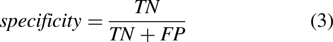
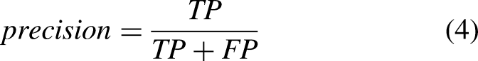
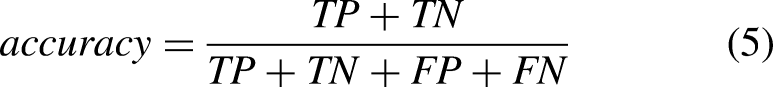
The performance of ML and DL methods was evaluated and compared. Moreover, the effect of the sensor location, sensor type, tasks, and activities was evaluated. Sensitivity (equation (2)), specificity (equation (3)), precision (equation (4)), accuracy (equation (5)), and F–score (equation (6)) were computed as follows: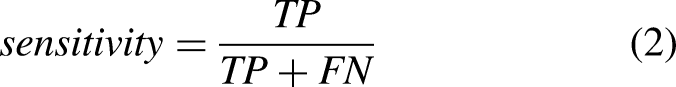

s e n s i t i v i t y = \frac{T P}{T P + F N}

(2)

s p e c i f i c i t y = \frac{T N}{T N + F P}

(3)

p r e c i s i o n = \frac{T P}{T P + F P}

(4)

a c c u r a c y = \frac{T P + T N}{T P + T N + F P + F N}

(5)

F - s c o r e = \frac{2 \cdot s e n s i t i v i t y \cdot p r e c i s i o n}{s e n s i t i v i t y + p r e c i s i o n}

(6)

where true positives (TP) and true negatives (TN) correspond to correctly recognized FoG and non-FoG windows, respectively; false positives (FP) and false negatives (FN) represent non-FoG windows classified as FoG and FoG windows classified as non-FoG, respectively. The F-score is computed as the harmonic mean of sensitivity and precision. It is preferred to accuracy in the case of unbalanced data, because accuracy can be misleading and often reflects high values simply for the prediction of the majority class. In addition, the AUROC was calculated, which measures the overall diagnostic capability of the prediction model. The classification metrics were calculated by selecting the classification threshold that minimizes the equal error rate. The latter represents the point on the ROC curve where sensitivity equals specificity. This is because a classification threshold of 0.5 is not appropriate in the case of very unbalanced classes.

Statistical tests were conducted to identify significant differences in the performance of different models (e.g., models trained with data from different sensors or combinations of sensors). To this end, ROC metrics (true positive rate and false positive rate) were calculated for each model using fixed threshold values (i.e., from 0 to 1 with 0.01 increments). The Mann-Whitney U-test was used to compare any differences in performance, with a statistical significance level of 0.05.

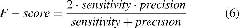
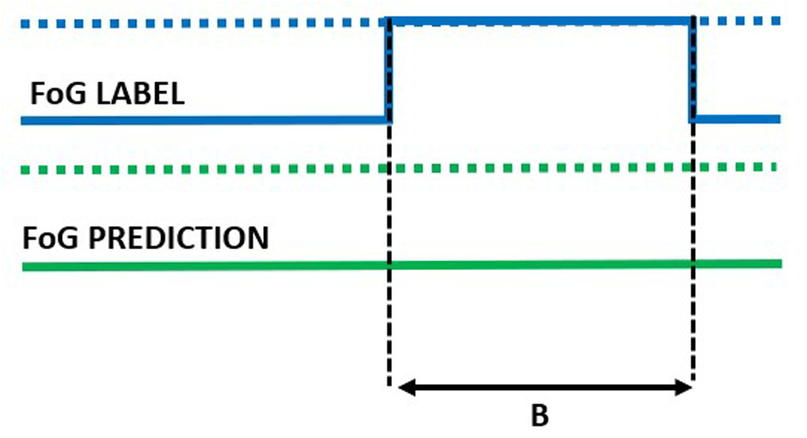
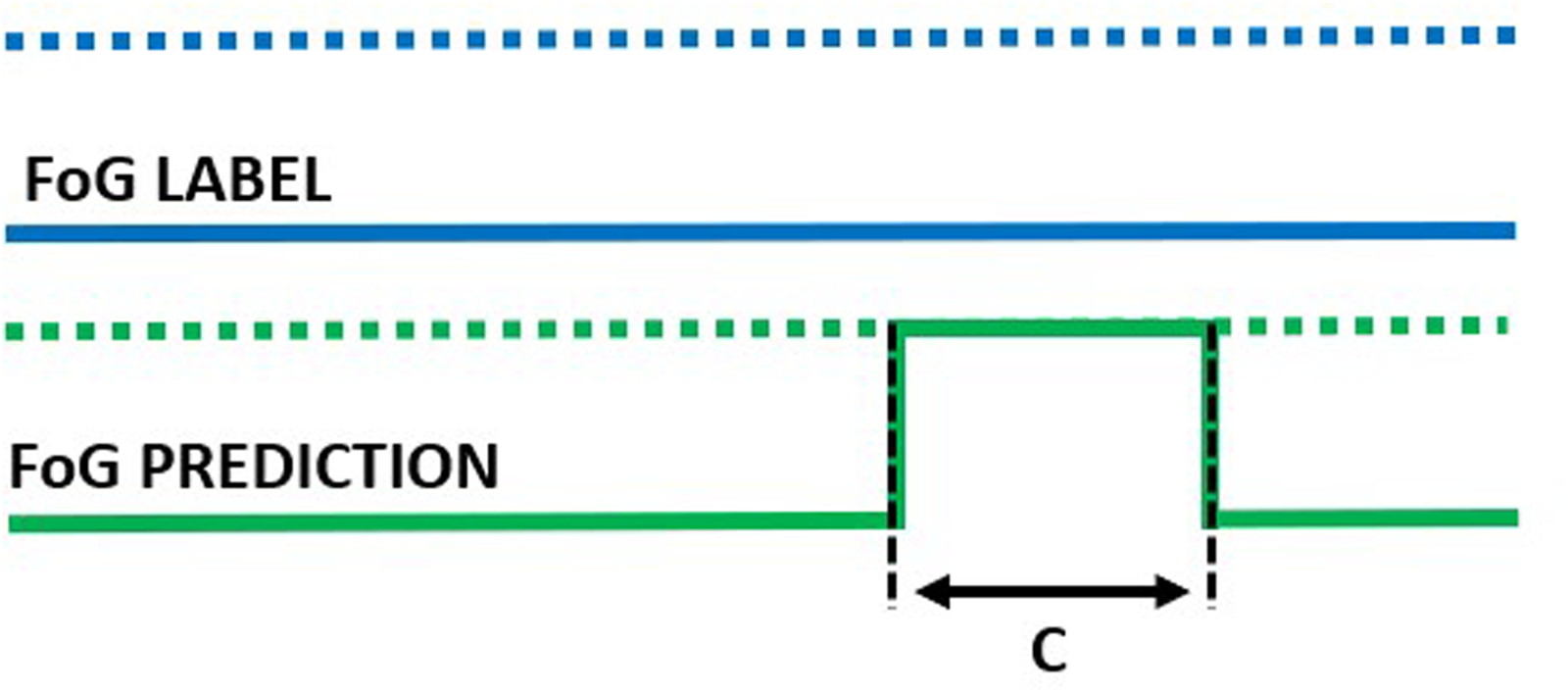
In addition to the window-level performance evaluation described above, episode-based performance was computed as follows. Starting from the model outputs, consecutive windows classified as FoG were aggregated to form a FoG episode. The overlap between real and detected FoG episodes was used to compute the following metrics. Real FoG episodes in which no windows were classified as FoG were considered missed/false negatives (Figure 7). On the other hand, FoG episodes detected by the model but not corresponding to real FoG were considered false episodes/false positives (Figure 8). The number of detected episodes (Figure 9) was computed. In this case, the detection delay was computed as the temporal difference (A) between the FoG onset and the beginning of the detected FoG ( i.e., end of the first window classified as FoG). The proportion of FoG episodes correponds to the proportion of detected/real FoG episodes (C/B). Finally, predicted FoG episodes (Figure 10) were identified as real episodes that were predicted before their actual occurrence. In this case, the prediction horizon was computed as the temporal distance (A) between the beginning of the detected FoG (corresponding to the end of the first window predicted as FoG) and the beginning of the real FoG episode (as identified by the clinical raters). Again, the proportion of FoG episodes detected can be calculated as C/B.

Figure 7.

Missed episode of duration B.

Figure 8.

False episode of duration C.

Figure 9.

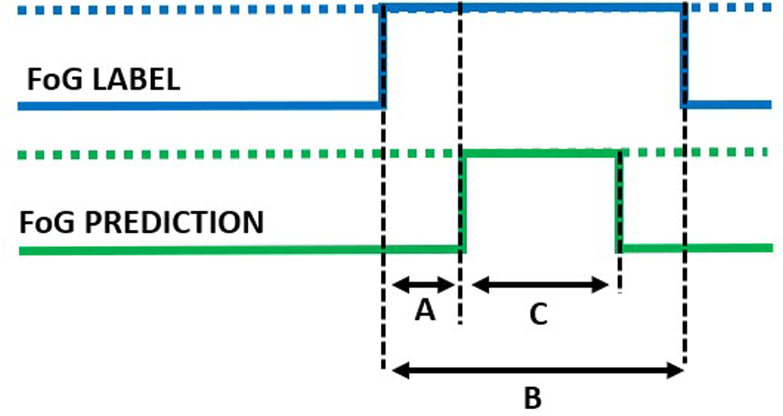
Detected episode. A: detection delay; B: true episode duration; C: detected episode duration.

Figure 10.

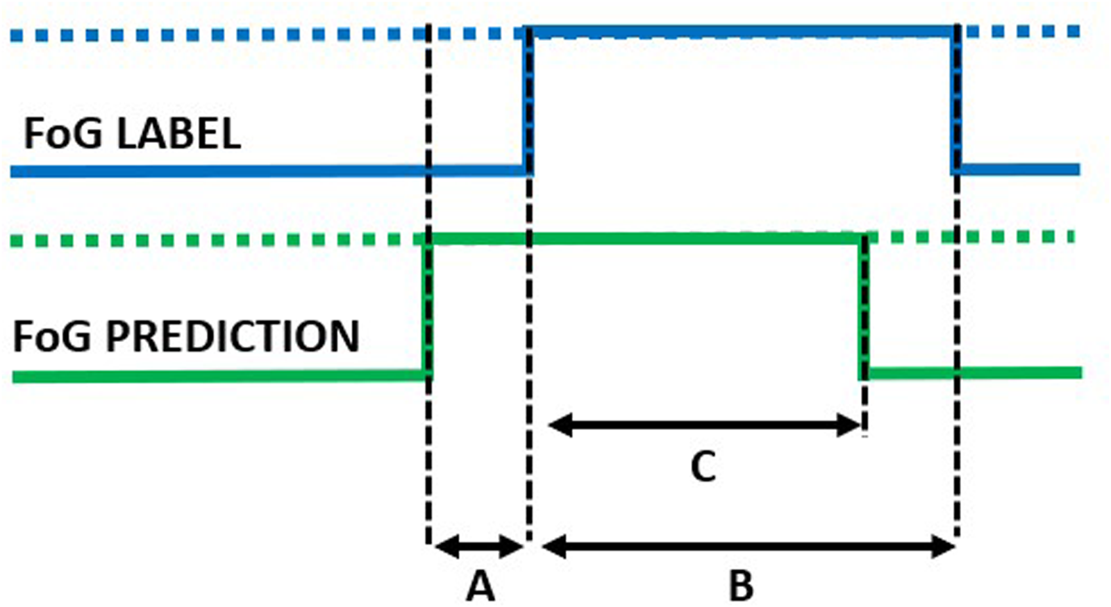
Predicted episode. A: prediction horizon; B: true episode duration; C: detected episode duration.

The experiments were performed on a computer with a 2.3 GHz processor, 16 GB RAM and 4 GB GPU. Pre- and post-processing were performed in Matlab (version R2023a), while ML and DL model training and optimization were carried out in Python (version 3.11.6), using keras (version 2.12.0) with tensorflow backend (2.12.0) and scikit-learn (version 1.2.2) packages.

Results

Demographic and clinical characteristics of the sample

Table 3 reports the demographic and clinical information of the subjects enrolled in this study.

Table 3.

Demographic and clinical information of patients enrolled.

	Average	STD	Min	Max
Age (years)	71.3	9.2	54	86
Disease duration (years)	10.8	6.0	4	25
H&Y	2.8	0.8	2	4
MDS-UPDRS part-I	17.3	4.6	10	27
MDS-UPDRS part-II	19.2	7.1	10	38
MDS-UPDRS part-III	38.7	14.4	18	69
FOG-Q	18.1	5.3	7	27
MOCA	21.3	3.8	15	29
FES-I	36.5	26.4	11	100
PDQ-8	14.2	6.8	3	29

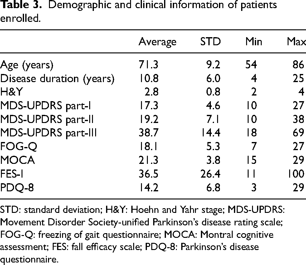
STD: standard deviation; H&Y: Hoehn and Yahr stage; MDS-UPDRS: Movement Disorder Society-unified Parkinson’s disease rating scale; FOG-Q: freezing of gait questionnaire; MOCA: Montral cognitive assessment; FES: fall efficacy scale; PDQ-8: Parkinson’s disease questionnaire.

Twenty-two participants (12 males and 10 females) were included in this study, with a mean age of 71.3 $\pm$ 9.2 years, disease duration of 10.8 $\pm$ 6.0 years, Hoehn and Yahr stage of 2.7 $\pm$ 0.8 , Movement Disorder Society modified version of the unified Parkinson’s disease rating scale part I 17.3 $\pm$ 4.6, part II 19.2 $\pm$ 7.1, and part III 38.7 $\pm$ 14.4 (18–69), FoG questionnaire 18.1 $\pm$ 5.3, Montreal cognitive assessment 21.3 $\pm$ 3.8, fall efficacy scale international 36.5 $\pm$ 26.4, PD questionnaire (PDQ-8) 14.2 $\pm$ 6.8. Participants were very satisfied with the wearable technology used for data acquisition. Specifically, the total QUEST score related to the devices was 38.2 $\pm$ 1.9 (min = 34, max = 40), with 40 being the highest score.

Data

Four wearable IMUs recorded three-axis acceleration and angular velocity signals from both ankles, lower back, and wrist, providing a total of 91.4 minutes of data. Figure 11 shows the total duration of each activity included in the experimental protocol. More than an hour of gait was recorded, comprising a similar duration of walking and turning. Static positions account for 18 minutes, where subjects were sit (5 minutes) or in an upright position (13 minutes). A total of 5 minutes of postural transitions (i.e., stand-to-sit and sit-to-stand) and 18 minutes of FoG were recorded.

Figure 11.

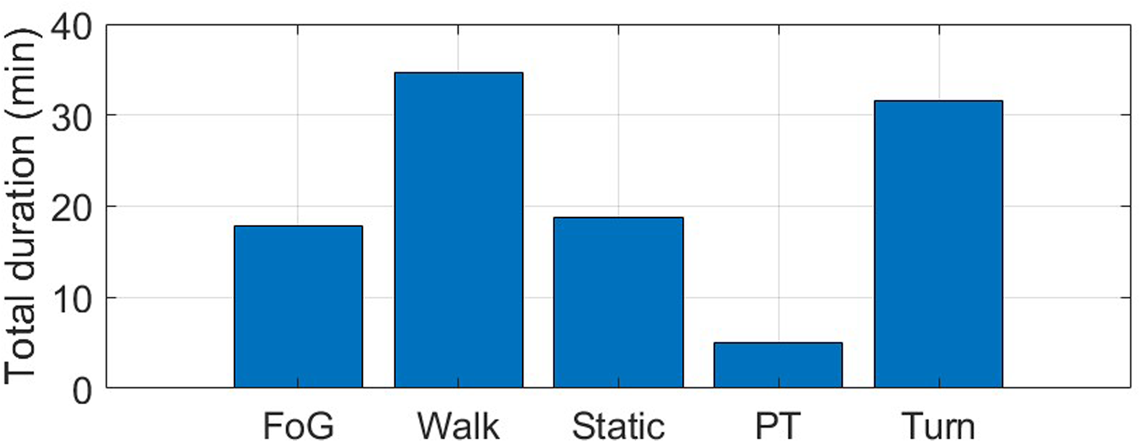
Total duration (min) of the different activities included in the experimental protocol. FoG: freezing of gait; Static: static postures, including stance and sit; PT: postural transitions, including sit-to-stand and stand-to-sit.

From the total sample of twenty-two subjects, sixteen (73%) experienced FoG during the experiments while six (27%) did not. Figure 12 reports the histogram of FoG episodes duration. A total of 101 episodes were recorded, with a mean duration of 9.2 s (median: 5.3 s, standard deviation: 16.9 s, interquartile range: 2.6 s–11.6 s, range: 0.6 s–108 s). Two episodes lasted more than 100 s, and manifested during 360-degree turn in two patients with an Hoehn & Yahr of 4. FoG severity was balanced across classes, with approximately 30% of mild FoG, and around 35% of moderate and severe FoG (Figure 13). More than 80% of FoG episodes manifested during turning, with only 10% of start hesitations and 10% of FoG during straight-line walking.

Figure 12.

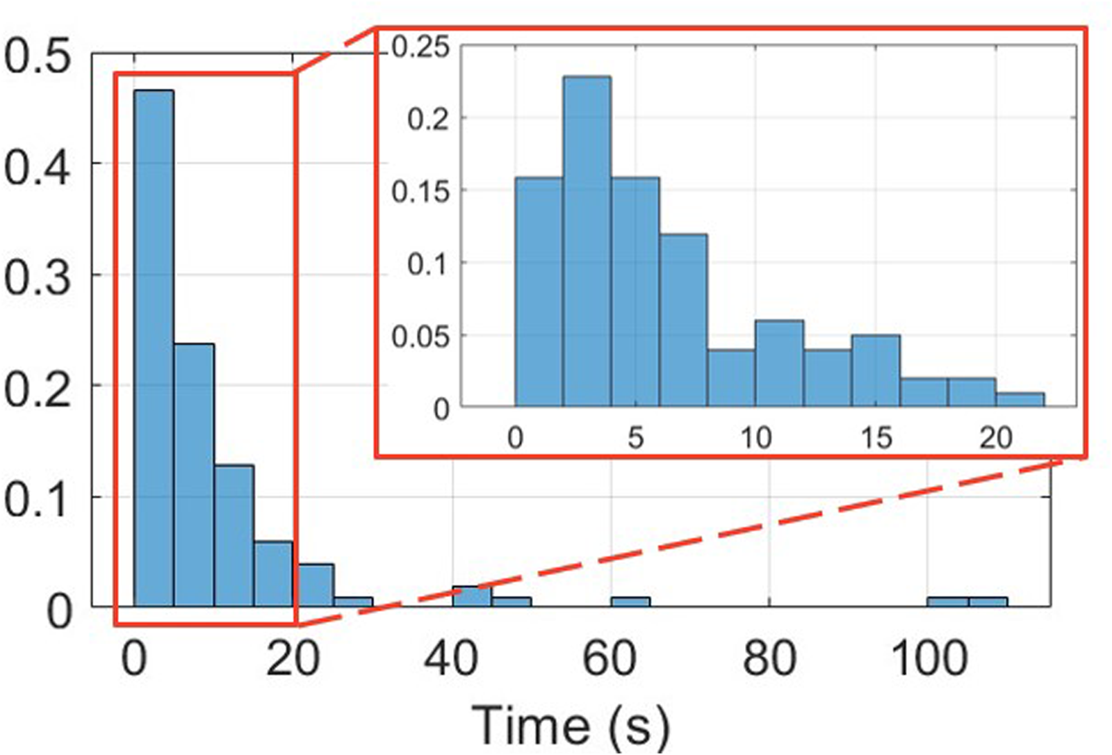
Normalized histogram of FoG episodes duration.

Figure 13.

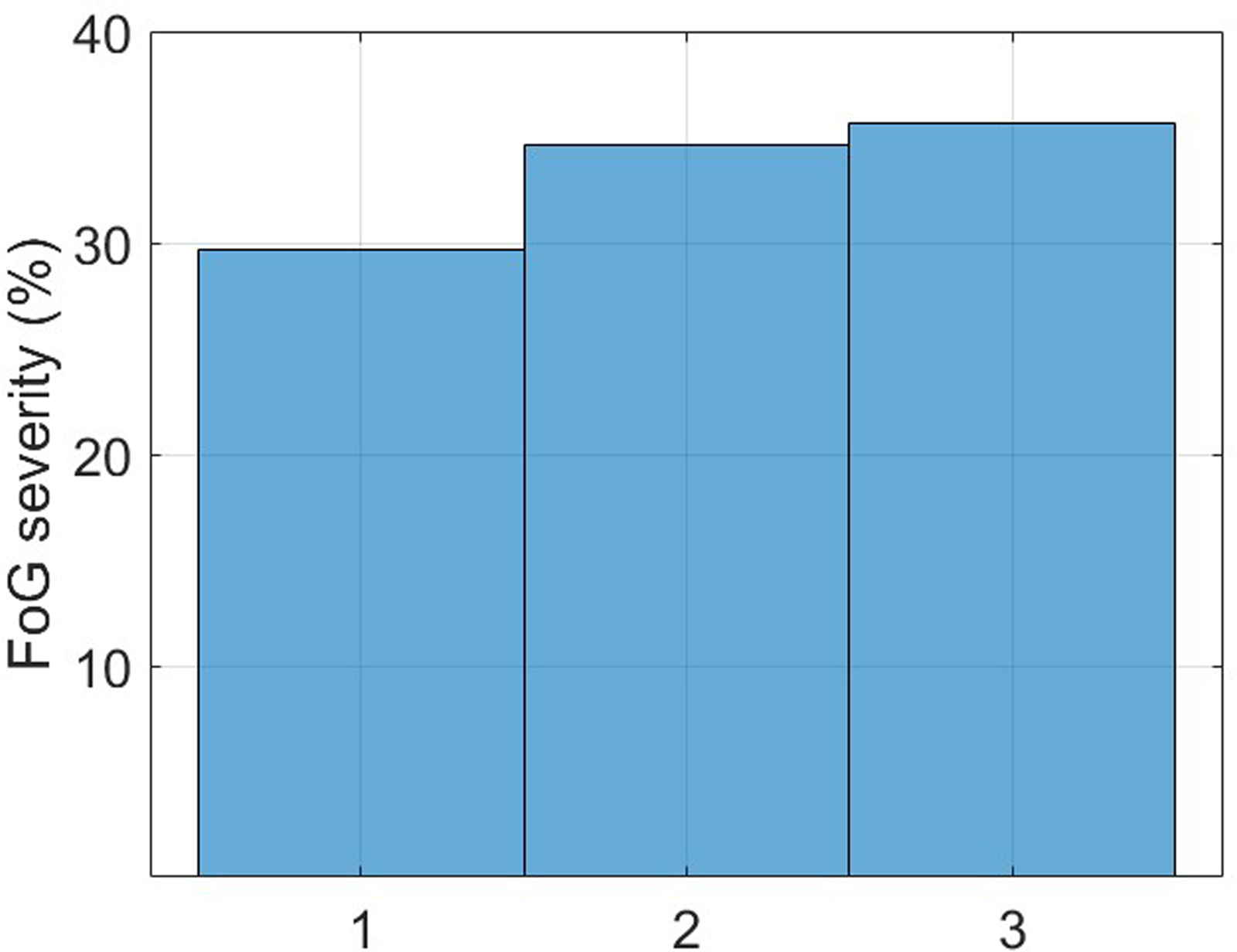
FoG episodes severity (1: shuffling forward with small steps, 2: trembling in place with alternating rapid knee movements, 3: complete akinesia without limbs or trunk movement).

Rater agreement

Raters 1 and 2 identified 125 and 99 episodes of FoG, respectively. After resolving the inconsistencies, they finally agreed in identifying 101 episodes. The ICC between the two raters was 0.80 for the number of FoG episodes and 0.88 for %TF, which show good-to-strong agreement between raters.^50,51 Interestingly, rater agreement varied across tasks, with strong agreement on the %TF during gait tasks (ICC = 0.80–0.92) and significantly lower agreement in the 360-degree task (ICC = 0.49). From the total number of video-recordings ( $n = 130$ ), both evaluators did not identify any FoG in 42.3% of cases ( $n = 55$ ). From the remaining recordings ( $n = 75$ ), the discrepancy in the total number of labelled FoG episodes was identified in 66.7% of cases ( $n = 50$ ). From the remaining records ( $n = 25$ ), a difference of more than 0.5 seconds in the onset of FoG was identified in 56% of cases ( $n = 14$ ). Of these, there was less than 80% overlap between the episodes identified by the two evaluators in 50% of the cases ( $n = 7$ ).

It is worth noting that in some cases, especially during turning, two different episodes of FoG occurred with a very short free interval and without a clear resume of the standard velocity and stride amplitude of patient’s gait. After having verified these particular conditions, clinical raters agreed to consider these episodes as a unique episode of FoG as this was considered the best choice from the clinical and algorithm training standpoints.

FoG detection performance

From the total number of participants, eleven were used for training and optimizing the ML models, five for validation, and six for test. This approach ensured subject independence across sets, providing more realistic estimates of model performance on unseen data. The training and validation sets did not significantly differ for age (70.8 $\pm$ 10.5, 68.2 $\pm$ 8.2, $p = 0.25$ ), Hoehn & Yahr stage (2.7 $\pm$ 0.9, 2.5 $\pm$ 0.6, $p = 0.93$ ), MDS-UPDRS-III (38.3 $\pm$ 13.1, 40.8 $\pm$ 18.8, $p = 0.68$ ) or FoG Questionnaire (18.9 $\pm$ 5.1, 20.8 $\pm$ 1.3, $p = 0.67$ ).

Table 4 reports the classification results of the feature-driven (i.e., extracted features input to a random forest algorithm) and data-driven (raw data input to a CNN) approaches on the validation set. The results are expressed in terms of mean and standard deviation over five iterations, to account for the effects of random weight and bias initialization across network layers. It is noteworthy that the metrics (e.g., mean and standard deviation) were calculated using the same data distribution for training, validation, and test. Data from all sensors were used at this stage. The data-driven DL model outperformed the feature-driven ML algorithm in all classification metrics. Overall, the DL approach provided an increase of 25.3% in F-score and 29.9% in AUROC. This demonstrates the superior performance of the data-driven approach, which automatically extracts and selects salient features capable of accurately detect FoG. It is worth noting that, despite very good performance in terms of sensitivity, specificity and AUROC, the low F-score indicates the difficulty in discarding false positives.

Table 4.

Classification results on the validation set.

Approach	Sensitivity	Specificity	Accuracy	F-score	AUROC
Feature-driven (RF)	0.409 $\pm$ 0.026	0.816 $\pm$ 0.006	0.784 $\pm$ 0.007	0.229 $\pm$ 0.015	0.613 $\pm$ 0.014
Data-driven (CNN)	0.852 $\pm$ 0.022	0.855 $\pm$ 0.021	0.854 $\pm$ 0.022	0.482 $\pm$ 0.043	0.912 $\pm$ 0.019

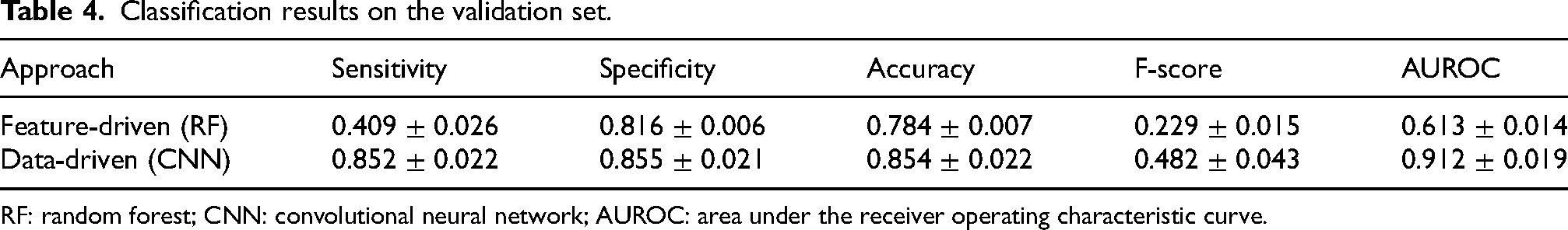
RF: random forest; CNN: convolutional neural network; AUROC: area under the receiver operating characteristic curve.

The effect of sensor location

Table 5 reports the classification performance of the data-driven algorithm for different sensor locations. At this stage, both acceleration and angular velocity signals were used for the analysis. Individually, sensors on the ankles were the best-performing, followed by the sensors on the lower back and the wrist. Further combining the sensors on both ankles, ankle and lower back, or ankle and wrist did not provide incremental performance, compared to the left-ankle only. The combination of all sensors provided the best results, with a slight improvement over the left-ankle sensor only. However, this performance improvement was not statistically significant ( $p = 0.10$ ). Thus, this single-sensor approach can represent a minimally invasive solution for FoG monitoring. It is worth noting the different performance of left and right ankle may be due to the different proportion of left and right turning directions. Specifically, while the 360 degree-turn was executed both clockwise and anti-clockwise, most 180 degree turns were in the anti-clock direction. This suggests that, during turning, the sensor placed on the internal leg (i.e., internal side of the turning) better capture the FoG pattern.

Table 5.

Classification results on the validation set based on sensor location.

Sensor location	Sensitivity	Specificity	Accuracy	F-score	AUROC
All	0.852 $\pm$ 0.022	0.855 $\pm$ 0.021	0.854 $\pm$ 0.022	0.482 $\pm$ 0.043	0.912 $\pm$ 0.019
Left-ankle	0.840 $\pm$ 0.013	0.842 $\pm$ 0.015	0.842 $\pm$ 0.015	0.456 $\pm$ 0.026	0.924 $\pm$ 0.010
Both ankles	0.815 $\pm$ 0.044	0.812 $\pm$ 0.044	0.812 $\pm$ 0.044	0.412 $\pm$ 0.067	0.902 $\pm$ 0.034
Right-ankle	0.811 $\pm$ 0.031	0.813 $\pm$ 0.034	0.813 $\pm$ 0.033	0.409 $\pm$ 0.054	0.911 $\pm$ 0.014
Lower-back	0.701 $\pm$ 0.064	0.700 $\pm$ 0.065	0.701 $\pm$ 0.065	0.276 $\pm$ 0.064	0.774 $\pm$ 0.065
Wrist	0.607 $\pm$ 0.057	0.606 $\pm$ 0.055	0.606 $\pm$ 0.056	0.197 $\pm$ 0.033	0.638 $\pm$ 0.007

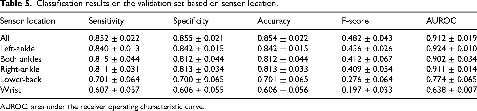
AUROC: area under the receiver operating characteristic curve.

The effect of sensor type

Table 6 reports the classification performance of the DL model based on different sensor types. The results refer to the sensor on the left ankle. The gyroscope sensor provided significantly better results ( $p < 0.001$ ). Overall, an increase of 8.9% in F-score and 3.1% in AUROC were registered. The comparison of Tables 5 and 6 shows that the accelerometer did not provide any significant contribution to FoG detection. The Mann-Withney U-test performed on the ROC curves confirmed that the combination of both sensors did not significantly improve classification performance ( $p = 0.21$ ), compared to the gyroscope sensor alone.

Table 6.

Classification results on the validation set based on sensor type.

Sensor type	Sensitivity	Specificity	Accuracy	F-score	AUROC
Accelerometer	0.784 $\pm$ 0.022	0.781 $\pm$ 0.023	0.781 $\pm$ 0.024	0.362 $\pm$ 0.031	0.889 $\pm$ 0.013
Gyroscope	0.837 $\pm$ 0.014	0.838 $\pm$ 0.014	0.838 $\pm$ 0.014	0.451 $\pm$ 0.024	0.920 $\pm$ 0.008

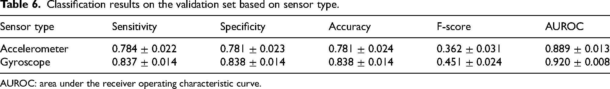
AUROC: area under the receiver operating characteristic curve.

Distinguishing FoG from various activities

Table 7 reports the classification performance in discriminating FoG from different activities. FoG can be easily distinguished from walking (AUROC 0.97), postural transitions (AUROC 0.95) and static positions (AUROC 0.93). On the other hand, discriminating FoG from turning represents a more complex task, proved by a net decrease in F-score and AUROC. The higher F-score observed when discriminating between FoG and postural transitions may be due to the fact that transitions are less represented than walk and static postures (see Figure 11). The proportion of negative instances and thus of possible false positives is reduced in this case.

Table 7.

Classification results on the validation set based on different activities.

Activity	Sensitivity	Specificity	Accuracy	F-score	AUROC
Walk	0.936 $\pm$ 0.008	0.936 $\pm$ 0.007	0.936 $\pm$ 0.007	0.801 $\pm$ 0.019	0.986 $\pm$ 0.003
Transition	0.908 $\pm$ 0.020	0.912 $\pm$ 0.020	0.909 $\pm$ 0.020	0.930 $\pm$ 0.015	0.948 $\pm$ 0.019
Static	0.879 $\pm$ 0.031	0.883 $\pm$ 0.025	0.882 $\pm$ 0.026	0.801 $\pm$ 0.041	0.934 $\pm$ 0.032
Turn	0.773 $\pm$ 0.008	0.769 $\pm$ 0.009	0.771 $\pm$ 0.008	0.687 $\pm$ 0.010	0.851 $\pm$ 0.008

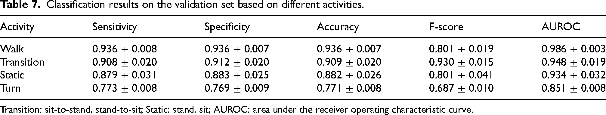
Transition: sit-to-stand, stand-to-sit; Static: stand, sit; AUROC: area under the receiver operating characteristic curve.

Classification results on the test set

Validation and test sets did not significantly differ for age (68.2 $\pm$ 8.2, 70.5 $\pm$ 7.6, $p = 0.36$ ), Hoehn & Yahr stage (2.5 $\pm$ 0.6, 2.7 $\pm$ 0.9, $p = 0.81$ ), MDS-UPDRS-III (40.8 $\pm$ 18.8, 38.7 $\pm$ 16.4, $p = 0.92$ ) or FoG Questionnaire (20.8 $\pm$ 1.3, 20.7 $\pm$ 6.4, $p = 0.67$ ). Table 8 compares the validation and test performance. No significant change is observed, with a slight reduction in AUROC and a consistent increase in F-score. The latter can be a result of a different class distribution among sets, with a larger FoG duration in the test set. Specifically, the validation and test sets comprised 185 and 327 seconds of FoG, respectively. Overall, the similar performance in the two sets proves the absence of over-fitting and the good generalization capability of the algorithm, which performs well on a new set of subjects. It is worth noting that the results refer to the gyroscope sensor placed on the left ankle.

Table 8.

Classification results on the validation and test sets. Results refer to the gyroscope sensor positioned on the left ankle.

Set	Sensitivity	Specificity	Accuracy	F-score	AUROC
Validation	0.837 $\pm$ 0.014	0.838 $\pm$ 0.014	0.838 $\pm$ 0.014	0.451 $\pm$ 0.024	0.920 $\pm$ 0.008
Test	0.823	0.824	0.823	0.628	0.909

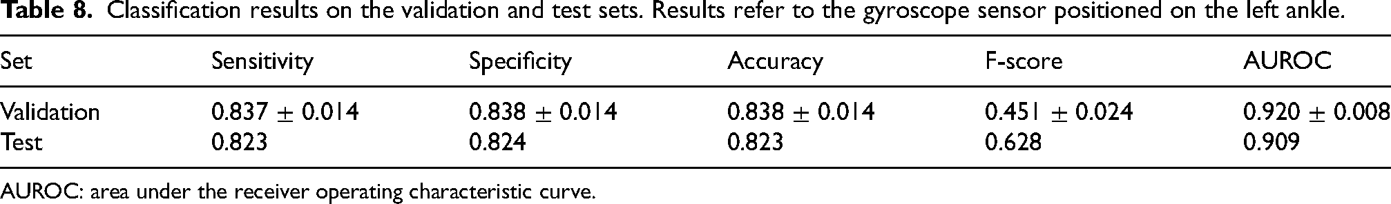
AUROC: area under the receiver operating characteristic curve.

Overall, 25% of episodes were predicted on average 2 s in advance from FoG onset, 25% were detected at onset, 37.5% were recognized with an average delay of 1 s, and 12.5% were not detected.

As far as concerns false FoG episodes, 65.3% of the recognized episodes were false positives. However, 23.4% of them represented isolated single-window episodes with adjacent non-FoG windows. The remaining false FoG episodes had a mean duration of 2.7 s, which is far lower than the mean duration of real FoG episodes (9.2 s). False FoG episodes mostly manifested during stance (46%) and turning (36%), while a small percentage occurred during straight walking (4%) and postural transitions (4%). This confirm the results reported in the previous section, i.e., very good capability in discriminating FoG from walk and postural transitions, and more difficulty in distinguishing FoG from turns and static upright positions. Specifically, false FoG episodes that manifested during static positions were shorter (2 s on average) than those occurring during turning (5.8 s on average). These results demonstrate the challenging gait pattern during turning, that can be confused with FoG.

Classification results on the independent datasets

Table 9 compares the FoG detection performance on the test set and the two external datasets. Results refer to the gyroscope sensor on the left ankle. It is worth noting that all the sets include new subjects, who were never assessed before by the model. Thus, all of them contribute to real performance estimates in unseen data.

Table 9.

Classification results on the test set and independent datasets. Results refer to the gyroscope sensor positioned on the left ankle. The results refer to the performance on the entire dataset.

Set	Sensitivity	Specificity	Accuracy	F-score	AUROC
Test (6 subjects)	0.826	0.825	0.825	0.632	0.909
O’Day dataset (7 subjects)²⁹	0.740	0.741	0.740	0.625	0.810
Multi-modal dataset (12 subjects)³¹	0.765	0.765	0.765	0.739	0.802

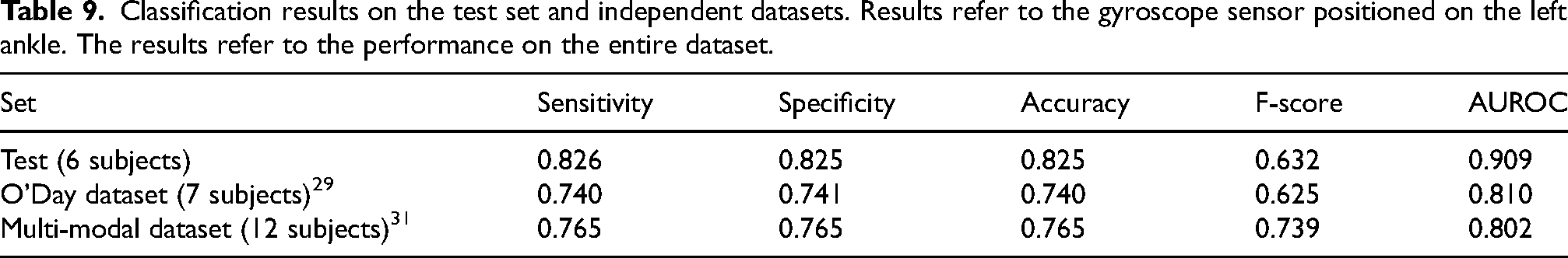
The sets differ for the subjects characteristics and the experimental procedures, together with a different amount of data. Specifically, the test set includes 6 subjects, with a total of 14 min of data (18% of FoG); the O’Day dataset²⁹ comprises 7 subjects, with a total of 89 min of data (24% FoG); the Multi-modal dataset³¹ includes 12 subjects with 222 min of data (40% FoG). Moreover, the set of performed activities is different, with additional ellipses and figures of eight tasks in O’Day et al.,²⁹ and walking through randomly placed obstacles in Guo et al.³¹ Indeed, the larger proportion of turning may have affected the performance, as previously discussed. Overall, AUROC decreases by 9.9–10.7% in the external datasets. However, the F-score is consistent, with 0.7% decrease in the O’Day dataset²⁹ and 10.7% increase in the Multi-modal dataset.³¹

In the O’Day dataset, 9.2% episodes were detected at onset, 26.2% were predicted on average 2.4 s before FoG onset, 56% were recognized with an average delay of 1.3 s, and 5% were not detected. As far as concerns false FoG episodes, 65.1% of the recognized episodes were false positives. However, 61.4% of them represented single-window episodes, which can be easily discarded. The remaining false FoG episodes had a mean duration of 1.8 s, which is far lower than the mean duration of real FoG episodes (7.8 s).

In the Multi-modal dataset, 11.6% episodes were detected at onset, 35.9% were predicted on average 2.1 s before FoG onset, 30.6% were recognized with an average delay of 2.1 s, and 12% were not detected. As far as concerns false FoG episodes, 39.6% of the recognized episodes were false positives. However, 44.8% of them represented single-window episodes, which can be easily discarded. The remaining false FoG episodes had a mean duration of 3 s, which is far lower than the mean duration of real FoG episodes (8.2 s).

It is worth noting that the F-score is generally low in all datasets, indicating a low precision value. To further investigate the relationship between sensitivity and precision, the area under the precision-recall curve was calculated, resulting in 0.669, 0.593 and 0.748 in the test set, O’Day and Multi-modal dataset, respectively. This confirms the difficulty of combining adequate sensitivity with good precision.

Figures 14 and 15 provide a visual representation of some predicted and timely detected FoG episodes, along with false positives. Data refer to the O’Day dataset. In Figure 14, two correctly detected FoG episodes are shown, along with three false positives.

Figure 14.

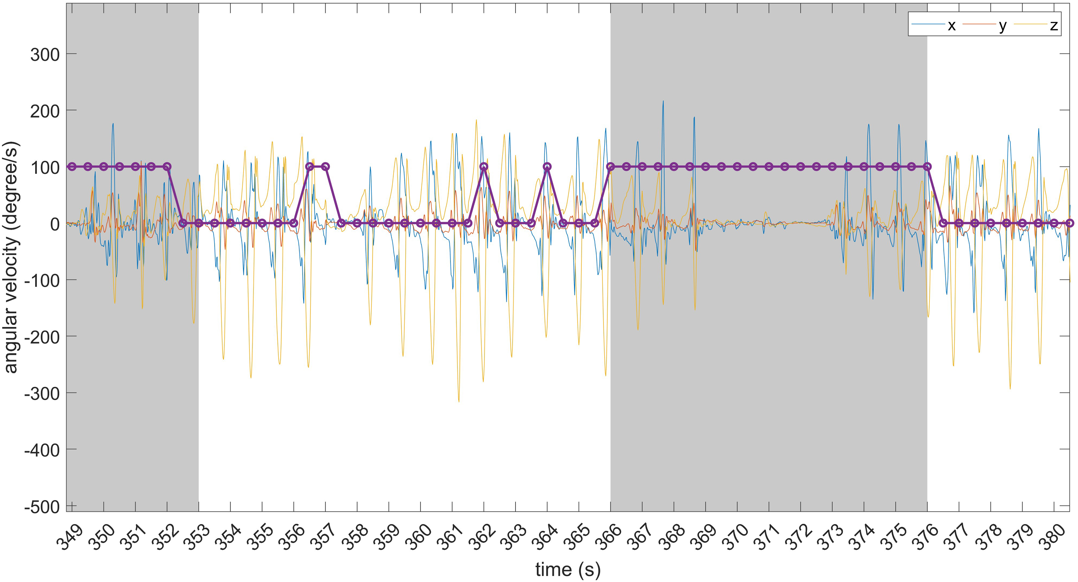
Examples of timely detected FoG episodes and false positives. The grey area identifies FoG events. From left to right: correctly detected FoG episode; false positive consisting of two consecutive windows; two isolated (single-window) false positives; timely detected FoG episode.

Figure 15.

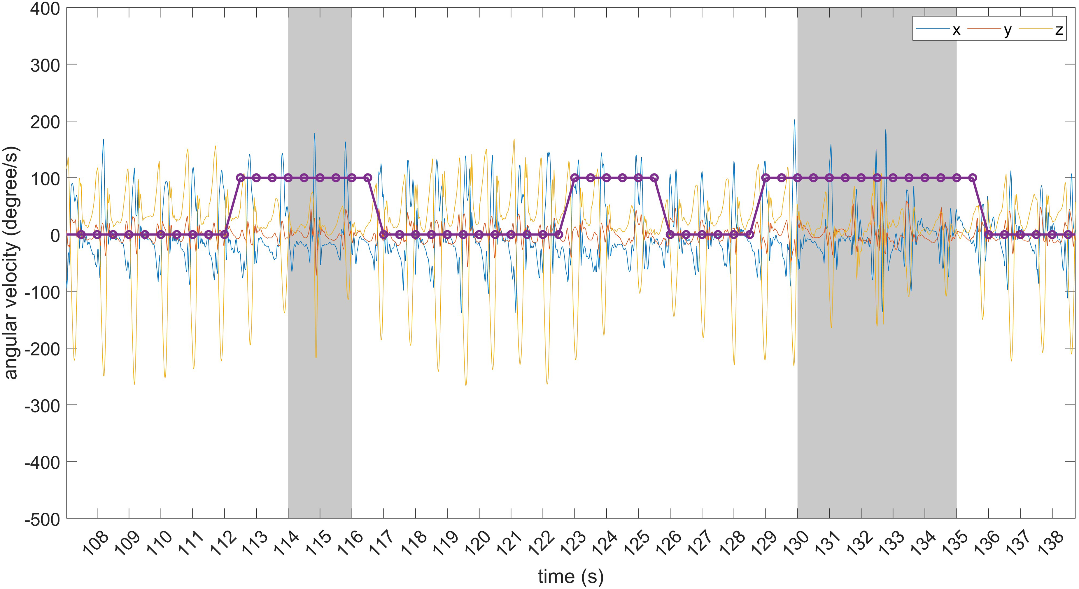
Examples of predicted FoG episodes and false positives. The grey area identifies FoG events. From left to right: predicted FoG episode; false positive consisting of six consecutive windows; predicted FoG episode.

Of these, one is made of two consecutive windows while the others are isolated (single-window) predictions. The latter can be discarded using some post-processing (e.g., majority voting over consecutive overlapped windows). Figure 15 shows two predicted FoG episodes, with different prediction horizons. As evident, FoG prediction starts before the real FoG occurrence and lasts for the entire FoG duration. On the other hand, the false positive is made of six consecutive windows and can not be discarded using post-processing techniques.

The results of the present study are in line with those of the original authors of the O’Day dataset.²⁹ When using a single sensor for FoG recognition, the ankle-mounted sensor performed best, with an AUROC between 0.60 and 0.80. This is in line with the AUROC of 0.81 obtained in this study. It is worth considering that O’Day et al.²⁹ trained and tested the model in a leave-one-subject-out validation, whereas in this work the entire dataset was used as an independent test. Regarding the Multi-modal dataset,³¹ the authors reported 0.756 sensitivity and 0.741 F-score when they used three accelerometers placed on both shins and lower back. This is in line with the 0.765 sensitivity and 0.739 F-score obtained in this study. However, while Guo et al.³¹ trained and tested the model in a leave-one-subject-out validation and used three sensors, in this work the entire dataset was used as an independent test and a single sensor was employed on the ankle.

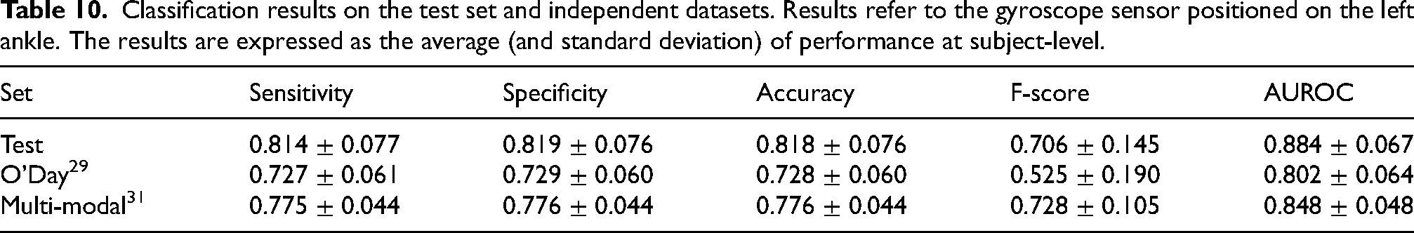
Table 10 reports the classification performance on the independent datasets, calculated at subject-level and expressed in terms of mean and standard deviation across subjects. The comparison of Tables 9 and 10 highlights no evident difference in performance, in terms of sensitivity, specificity, accuracy, and AUROC. On the other hand, the F score is influenced by the different evaluation procedures. In particular, subject-level performance leads to an increase of the F-score in the test set and a decrease of the F-score in the O’Day dataset, while it shows similar values for the Multi-modal dataset.

Table 10.

Classification results on the test set and independent datasets. Results refer to the gyroscope sensor positioned on the left ankle. The results are expressed as the average (and standard deviation) of performance at subject-level.

Set	Sensitivity	Specificity	Accuracy	F-score	AUROC
Test	0.814 $\pm$ 0.077	0.819 $\pm$ 0.076	0.818 $\pm$ 0.076	0.706 $\pm$ 0.145	0.884 $\pm$ 0.067
O’Day²⁹	0.727 $\pm$ 0.061	0.729 $\pm$ 0.060	0.728 $\pm$ 0.060	0.525 $\pm$ 0.190	0.802 $\pm$ 0.064
Multi-modal³¹	0.775 $\pm$ 0.044	0.776 $\pm$ 0.044	0.776 $\pm$ 0.044	0.728 $\pm$ 0.105	0.848 $\pm$ 0.048

Discussion

Two independent raters meticulously annotated the beginning and end of FoG episodes, reconciling any disparities in counts, durations, and onset of FoG. Additionally, the raters classified participants’ activities, encompassing static postures, postural transitions, walking, and turning. Overall, this annotation approach not only holds significance for prospective applications in automatic activity segmentation but can also contributes substantially to the understanding of FoG characteristics. To ensure a comprehensive data collection process, a multi-sensor system was deployed, comprising four IMUs equipped with 3-axis accelerometers and 3-axis gyroscopes strategically placed on the ankles, lower back, and wrist. This systematic configuration enables the examination of each sensor’s contribution, the identification of optimal sensor locations, and the formulation of sensor combinations that optimally capture FoG characteristics. Finally, participants underwent various gait tasks under triggering conditions, including motor and cognitive dual-tasks, negotiation of obstacles, and execution of 360-degree turns. The complete dataset, including the sensor data and both the final and intermediate annotations from the raters, will be made open-source in a dedicated publication, where the dataset will serve as the primary outcome and enable future research.

The data-driven DL algorithm outperformed the feature-driven ML algorithm. It is worth noting that the latter (random forest) is a well-known algorithm, which has proven robust in a large variety of tasks, including FoG detection.^12,52,53 Moreover, the features extracted in this study were selected from similar works.^23,54–56 Finally, the processing pipeline comprised feature selection and data augmentation, which demonstrated to improve performance.^57,58 The superior performance of the DL model confirms the findings of similar recent studies, where a consistent performance improvement was registered using DL algorithms.^{26,27,36,59,60} Indeed, data-driven neural networks can find salient hidden patterns, and extract and select the most significant features for the specific classification task.

The combination of sensors on different positions proved to be beneficial to the final performance. However, the use of a single sensor on the ankle provides similar performance to the combination of all inertial modules, while reducing the complexity of the sensor setup. Thus, this can represent a minimally invasive solution for accurate FoG monitoring. When using a single sensor, the present results are in line with those of related studies,^29,59,61 suggesting that the ankle is the best position for FoG detection. However, when using multiple body-worn sensors, O’Day et al.²⁹ found that the combination of sensors on the ankle and lower back provides better performance than the ankle sensor only. In Li et al.,⁵⁹ the ankle-mounted sensor provided similar performance than the combination of ankle, thigh, and back. In Mesin et al.⁶² the sensor on the ankle provided similar results than the combination of sensors on the ankle and back. The heterogeneity of sample, experimental procedures, and findings does not allow to identify the best single-sensor or sensor-combination setting. Furthermore, the results need to be contextualized, as classification performance depends on several factors, including the size of the dataset, the number of FoG events and the total duration of the FoG, the number and heterogeneity of subjects, the heterogeneity of the activities included, the pre-processing steps and the model selection. Interestingly, the results of the present study suggest that the performance achieved by a single sensor mounted on the ankle is dependent on the direction of turning. From the perspective of a general FoG detection system, sensors on both ankles may provide a more robust solution that is less sensitive to turning direction.

At present, only few studies have evaluated the performance of unsupervised FoG detection methods in daily life. In Mancini et al.,²⁸ three sensors were positioned on both ankles and the lower back, continuously recording data for a week. In Salomon et al.,²⁶ data were collected over 7 days using a single device mounted on the lower back. Finally, in Zoetewei et al.,⁷ two sensors placed on the shoes monitored FoG and provided on-demand feedback. Again, lower limbs and the lower back seem to be the preferred choice for continuous FoG monitoring in unsupervised settings.

The type of sensor affected the final performance. Specifically, the gyroscope performed better than the accelerometer. This is an interesting result, since some large and commonly used datasets^23,32,55 do not include gyroscope recordings. It is worth noting that the results refer to the sensor on the ankle, where wide rotational movements are recorded during walking. Using a single sensor on the lower back may provide different results, as high angular velocity values can be observed only during turning.

Few studies have compared the ability to distinguish FoG from different activities, confirming that FoG can be differentiated across different medication states and FoG-provoking tasks.^23,26,27,63 Consistent with these findings, our results demonstrated that walking, static postures, and postural transitions do not represent a major challenge. On the other hand, the gait patterns generated during turning impaired classification algorithms performance, in line with recent research.²⁷ This is an important finding and the topic for future studies, as most FoG episodes manifest during turning.⁴³ However, most studies grouped all activities different from FoG to form the “non-FoG” class, and few considered walking and turning activities as part of the “gait” class. This study suggests that activities should be better characterized. In particular, turning should be better represented in the experimental protocols and carefully labelled,²⁶ as it may significantly affect detection performance.

The results on the test set showed good generalization ability, with similar performance to the validation set. Moreover, the results at the episode level complemented those at the single-window level. In fact, a sensitivity of 82% was obtained at the window level, but 94% of episodes were recognized correctly. This shows that window-level performance does not provide a complete picture of FoG detection performance.

False positives still represent a major challenge in the development of FoG recognition algorithms. In the present study, a generally low F-score between 0.525 and 0.728 was found in the different datasets, together with an area under the precision-recall curve between 0.593 and 0.748. This demonstrates the difficulty of achieving high sensitivity and good precision. As the sensitivity increases, so does the false alarm rate, to the point where precision can be significantly impaired, compromising the ability to use the algorithm in real-world contexts. Indeed, it is necessary to reduce the number of false alarms, which can be annoying for patients when applying on-demand cueing strategies in daily life. Overall, it is clear that an acceptable compromise between sensitivity and false-positive rate must be carefully chosen. Furthermore, as the results suggest, post-processing methods can be used to discard isolated false positives. This can be done by applying majority voting on multiple overlapping windows, thus detecting FoG only when a certain number of consecutive windows are classified as FoG. On the one hand, this will improve the precision of the model. On the other hand, the sensitivity will decrease slightly, the prediction horizon will be reduced and the detection delay will increase. These considerations highlight the need for a careful evaluation of classification performance at both the window and episode level in order to provide a robust detection system that is ready to operate under real-world conditions.

For the first time, we performed a comprehensive cross-dataset test aimed at real performance estimation of the FoG recognition model. Testing the model on two external datasets resulted in generally lower performance in terms of AUROC. However, the rate of FoG episodes detected and false positives were consistent with those obtained on the main dataset. It is worth noting that the datasets differ in terms of sample, sensor setting, experimental procedures, and environment. Furthermore, the precise methods for clinical labelling of FoG episodes may differ in different datasets. Although it is not possible to control for this difference,⁶⁴ the results obtained, in line with those of the original authors, suggest a good ability to generalize to external datasets.

In view of an online, closed-loop wearable cueing system, real-time applications of the algorithm should be explored. Recent studies have shown potential for reducing FoG episodes, however, fast and lightweight algorithms are still needed for real-time implementation on resource-constrained devices such as wearables.^7,65 In this context, the DL model is light (35 KB memory, 8.3 K parameters) and very fast (60 ms for classification of a single window), and little pre-processing is needed (i.e., mean-removal). Moreover, the small slide of 0.5 s ensures timely data analysis and increases the possibility for timely intervention. The results of the test set demonstrated that more than half of FoG episodes were detected at onset and even predicted few seconds before the actual occurrence. The remaining episodes were detected on average after 1 s from FoG onset, and only 12% were missed. These results put the basis for future on-device implementation of the DL model, which can timely trigger some sort of somatosensory stimuli (auditory, visual, tactile).^6,66

Although this study has provided valuable insights, there are some limitations to acknowledge. Despite the number of participants included in this study is higher than most FoG datasets,^{29,31,32,55,67} the number of recorded FoG episodes (101 FoG episodes) is reduced compared to 211 episodes,²⁹ 334 episodes,³¹ 180 episodes,⁶⁷ 237 episodes,³² and more than 1000 episodes^23,26,55 registered in previous studies. This is due to the designed experimental procedures, producing a total recording time of few minutes per subject. Furthermore, of the twenty-two subjects enrolled in this study, only sixteen manifested FoG. As FoG varies widely between individuals, the design of a general detection system is challenging and limits the ability to draw definitive results and make accurate comparisons. The use of a more comprehensive dataset, such as DeFOG or transcranial direct current stimulation (tDCS),²⁶ could improve results by enabling the application of techniques such as transfer learning. Finally, the resampling of videos at 10 fps, while improving the clinical rating in terms of agreement and time, could have slightly affected the precision of the exact moment of start and end of FoG episodes, if compared to a video sampled at 30 or even 60 fps. In line with related works,^29,31,32 subjects were assessed in the OFF condition, to increase the probability of FoG manifestation. This does not allow to assess the effect of medication on the algorithm performance. Interestingly, a recent study²⁷ found that models trained on a specific medication state can generalize to unseen states. This study simulated free-living situations by asking patients to perform different tasks and activities. However, free-living movements (e.g., daily activities) are much more heterogeneous than those detected during standardized tasks. Moreover, the severity of FoG during laboratory assessment does not necessarily represent that of daily life.²⁶ Finally, data from QUEST to evaluate patients satisfaction with the devices is of limited generalizability due to the laboratory setting and the presence of investigators who helped patients putting sensors on and off. Therefore, future work should establish the reliability of the proposed approach to data measured in free-living situations or during the execution of complex real-world activities, as demonstrated in May et al.⁶⁸

Footnotes

Acknowledgements

This work was partially supported by the European Union under the Italian National Recovery and Resilience Plan (NRRP) of NextGenerationEU, with particular reference to the partnership on “Telecommunications of the Future” (PE00000001 - program “RESTART”) and the PRIN 2022 project “WE.SMOOTH.PD” (Grant 2022EJM345); the Brain Research Foundation Verona Onlus; FSE Projects under Grant 1695-0013-1463-2019.

ORCID iDs

Luigi Borzì

Florenc Demrozi

Ruggero Angelo Bacchin

Cristian Turetta

Giulio Balestro

Alessandro Picelli

Graziano Pravadelli

Gabriella Olmo

Stefano Tamburin

Carlo Alberto Artusi

Funding

The author(s) received no financial support for the research, authorship and/or publication of this article.

Declaration of conflicting interests

The author(s) declared no potential conflicts of interest with respect to the research, authorship, and/or publication of this article.

Data availability

Data that support the findings of this study will be made available through a public repository. At present, data are available upon reasonable request from the corresponding author. The convolutional neural network developed in this study is available at .

References

Pan

Tang

, et al. Global trends in the incidence, prevalence, and years lived with disability of parkinson’s disease in 204 countries/territories from 1990 to 2019. Front Public Health 2021; 9: 776847.

Bloem

Okun

Klein

. Parkinson’s disease. Lancet 2021; 397: 2284–2303.

Gao

Liu

Tan

, et al. Freezing of gait in parkinson’s disease: pathophysiology, risk factors and treatments. Transl Neurodegener 2020; 9: 12.

Herman

Barer

Bitan

, et al. A meta-analysis identifies factors predicting the future development of freezing of gait in parkinson’s disease. NPJ Parkinsons Dis 2023; 9: 158.

Cui

Lewis

SJG

. Future therapeutic strategies for freezing of gait in Parkinson’s disease. Front Hum Neurosci 2021; 15: 741918.

Ginis

Nackaerts

Nieuwboer

, et al. Cueing for people with parkinson’s disease with freezing of gait: a narrative review of the state-of-the-art and novel perspectives. Ann Phys Rehabil Med 2018; 61: 407–413.

Zoetewei

Herman

Ginis

, et al. On-demand cueing for freezing of gait in parkinson’s disease: a randomized controlled trial. Mov Disord 2024; 39: 876–886.

Barthel

Mallia

Debû

, et al. The practalities of assessing freezing of gait. J Parkinsons Dis 2016; 6: 667–674.

Mancini

Bloem

Horak

, et al. Clinical and methodological challenges for assessing freezing of gait: future perspectives. Mov Disord 2019; 34: 783–790.

10.

Giladi

Tal

Azulay

, et al. Validation of the freezing of gait questionnaire in patients with parkinson’s disease. Mov Disord 2009; 24: 655–661.

11.

Hulzinga

Nieuwboer

Dijkstra

, et al. The new freezing of gait questionnaire: unsuitable as an outcome in clinical trials? Mov Disord Clin Pract 2020; 7: 199–205.

12.

Pardoel

Kofman

Nantel

et al. Wearable-sensor-based detection and prediction of freezing of gait in Parkinson’s disease: a review. Sensors 2019; 19: 5141.

13.

Channa

Popescu

Ciobanu

. Wearable solutions for patients with Parkinson’s disease and neurocognitive disorder: a systematic review. Sensors 2020; 20: 2713.

14.

Huang

. Recent trends in wearable device used to detect freezing of gait and falls in people with Parkinson’s disease: a systematic review. Front Aging Neurosci 2023; 15: 1119956.

15.

Mei

Desrosiers

Frasnelli

. Machine learning for the diagnosis of parkinson’s disease: a review of literature. Front Aging Neurosci 2021; 13: 633752.

16.

Mirza

Wang

, et al. Machine learning and integrative analysis of biomedical big data. Genes 2019; 10: 87.

17.

Sarker

. Deep learning: a comprehensive overview on techniques, taxonomy, applications and research directions. SN Comput Sci 2021; 2: 1–20.

18.

Alzubaidi

Zhang

Humaidi

, et al. Review of deep learning: concepts, CNN architectures, challenges, applications, future directions. J Big Data 2021; 8: 53.

19.

Christ

Braun

Neuffer

, et al. Time series feature extraction on basis of scalable hypothesis tests (tsfresh–a python package). Neurocomputing 2018; 307: 72–77.

20.

Van Der Donckt

Deprost

, et al. tsflex: flexible time series processing & feature extraction. SoftwareX 2022; 17: 100971.

21.

Chandrabhatla

Pomeraniec

Ksendzovsky

. Co-evolution of machine learning and digital technologies to improve monitoring of parkinson’s disease motor symptoms. NPJ Digit Med 2020; 5: 32.

22.

Sigcha

Borzì

Amato

, et al. Deep learning and wearable sensors for the diagnosis and monitoring of Parkinson’s disease: a systematic review. Expert Syst Appl 2023; 229: 120541.

23.

Reches

Dagan

Herman

, et al. Using wearable sensors and machine learning to automatically detect freezing of gait during a fog-provoking test. Sensors 2020; 20: 4474.

24.

Giannakopoulou

Roussaki

Demestichas

. Internet of things technologies and machine learning methods for parkinson’s disease diagnosis, monitoring and management: A systematic review. Sensors 2022; 22: 1799.

25.

Moreau

Rouaud

Grabli

, et al. Overview on wearable sensors for the management of parkinson’s disease. NPJ Parkinsons Dis 2023; 9: 153.

26.

Salomon

Gazit

Ginis

, et al. A machine learning contest enhances automated freezing of gait detection and reveals time-of-day effects. Nat Commun 2024; 15: 4853.

27.

Yang

Filtjens

Ginis

, et al. Freezing of gait assessment with inertial measurement units and deep learning: effect of tasks, medication states, and stops. J Neuroeng Rehabil 2024; 21: 24.

28.

Mancini

Shah

Stuart

, et al. Measuring freezing of gait during daily-life: an open-source, wearable sensors approach. J Neuroeng Rehabil 2021; 18: 1.

29.

O’Day

Lee

Seagers

, et al. Assessing inertial measurement unit locations for freezing of gait detection and patient preference. J Neuroeng Rehabil 2022; 19: 20.

30.

Elbatanouny

Kleanthous

Dahrouj

, et al. Insights into Parkinson’s disease-related freezing of gait detection and prediction approaches: a meta analysis. Sensors 2024; 24: 3959.

31.

Guo

Huang

Zhang

, et al. High-accuracy wearable detection of freezing of gait in parkinson’s disease based on pseudo-multimodal features. Comput Biol Med 2022; 146: 105629.

32.

Bächlin

Plotnik

Roggen

, et al. Wearable assistant for parkinson’s disease patients with the freezing of gait symptom. IEEE Trans Inf Technol Biomed 2010; 14: 436–446.

33.

Ribeiro De Souza

Miao

Ávila De Oliveira

, et al. A public data set of videos, inertial measurement unit, and clinical scales of freezing of gait in individuals with parkinson’s disease during a turning-in-place task. Front Neurosci 2022; 16: 832463.

34.

Borzì

Sigcha

Olmo

. Context recognition algorithms for energy-efficient freezing-of-gait detection in Parkinson’s disease. Sensors 2023; 23: 4426.

35.

Borzì

Sigcha

Rodríguez-Martín

, et al. Real-time detection of freezing of gait in Parkinson’s disease using multi-head convolutional neural networks and a single inertial sensor. Artif Intell Med 2023; 135: 102459.

36.

Sigcha

Borzì

Olmo

. Deep learning algorithms for detecting freezing of gait in Parkinson’s disease: a cross-dataset study. Expert Syst Appl 2024; 255: 124522.

37.

Postuma

Berg

Stern

, et al. Mds clinical diagnostic criteria for parkinson’s disease. Mov Disord 2015; 30: 1591–1601.

38.

Nieuwboer

Rochester

Herman

, et al. Reliability of the new freezing of gait questionnaire: agreement between patients with parkinson’s disease and their carers. Gait Posture 2009; 30: 459–463.

39.

Demrozi

Turetta

Kindt

, et al. A low-cost wireless body area network for human activity recognition in healthy life and medical applications. IEEE Trans Emerg Top Comput 2023; 11: 839–850.

40.

Turetta

Demrozi

Pravadelli

. A freely available system for human activity recognition based on a low-cost body area network. In: 2022 IEEE 46th annual computers, software, and applications conference (COMPSAC). IEEE, pp.395–400.

41.

Louise Demers

RWL

Ska

. Development of the quebec user evaluation of satisfaction with assistive technology (quest). Assist Technol 1996; 8: 3–13.

42.

Giladi

Nieuwboer

. Understanding and treating freezing of gait in parkinsonism, proposed working definition, and setting the stage. Mov Disord 2008; 23: 423–425.

43.

Schaafsma

Balash

Gurevich

, et al. Characterization of freezing of gait subtypes and the response of each to levodopa in parkinson’s disease. Eur J Neurol 2003; 10: 391–398.

44.

Gavriliuc

Paschen

Andrusca

, et al. Clinical patterns of gait freezing in parkinson’s disease and their response to interventions: an observer-blinded study. Parkinsonism Relat Disord 2020; 80: 175–180.

45.

Ribeiro

Cachitas

Maode Ferro

, et al. Python video annotator, 2019. https://github.com/video-annotator/pythonvideoannotator.

46.

Naghavi

Wade

. Towards real-time prediction of freezing of gait in patients with Parkinson’s disease: a novel deep one-class classifier. IEEE J Biomed Health Inform 2022; 26: 1726–1736.

47.

Ding

Peng

. Minimum redundancy feature selection from mucroarray gene expression data. J Bioinform Comput Biol 2005; 3: 185–205.

48.

Chawla

Bowyer

Hall

, et al. Smote: synthetic minority over-sampling technique. J Artif Int Res 2002; 16: 321–357.

49.

Jindong

Yiqiang

Shuji

, et al. Deep learning for sensor-based activity recognition: a survey. Pattern Recogn Lett 2019; 119: 3–11.

50.

Aggarwal

Ranganathan

. Common pitfalls in statistical analysis: the use of correlation techniques. Perspect Clin Res 2016; 7: 187–190.

51.

Portney

Watkins

, et al. Foundations of clinical research: applications to practice vol. 892. NJ: Pearson/Prentice Hall Upper Saddle River, 2009.

52.

San-Segundo

Navarro-Hellín

Torres-Sánchez

, et al. Increasing robustness in the detection of freezing of gait in Parkinson’s disease. Electronics 2019; 8: 119.

53.

Sigcha

Borzì

Pavón

, et al. Improvement of performance in freezing of gait detection in Parkinson’s disease using transformer networks and a single waist-worn triaxial accelerometer. Eng Appl Artif Intell 2022; 116: 105482.

54.

Mazilu

Hardegger

Zhu

, et al. Online detection of freezing of gait with smartphones and machine learning techniques. In: 2012 6th international conference on pervasive computing technologies for healthcare (PervasiveHealth) and workshops, pp.123–130.

55.

Rodríguez-Martín

Samà

Pérez-López

, et al. Home detection of freezing of gait using support vector machines through a single waist-worn triaxial accelerometer. PLoS ONE 2017; 12: 1–26.

56.

Borzì

Olmo

Artusi

, et al. Detection of freezing of gait in people with Parkinson’s disease using smartphones. In: 2020 IEEE 44th Annual Computers, Software, and Applications Conference (COMPSAC), 2020, pp.625–635.

57.

Pfister

FMJ

Pichler

, et al. Data augmentation of wearable sensor data for parkinson’s disease monitoring using convolutional neural networks. In: Proceedings of the 19th ACM international conference on multimodal interaction, ACM, p.216–220.

58.

Samà

Rodríguez-Martín

Pérez-López

, et al. Determining the optimal features in freezing of gait detection through a single waist accelerometer in home environments. Pattern Recogn Lett 2018; 105: 135–143.

59.

Yao

Wang

, et al. Improved deep learning technique to detect freezing of gait in Parkinson’s disease based on wearable sensors. Electronics 2020; 9: 1919.

60.

Ghayvat

Awais

Geddam

, et al. Aicarepwp: deep learning-based novel research for freezing of gait forecasting in parkinson. Comput Methods Programs Biomed 2024; 254: 108254.

61.

Ashfaque Mostafa

Soltaninejad

McIsaac

, et al. A comparative study of time frequency representation techniques for freeze of gait detection and prediction. Sensors 2021; 21: 6446.

62.

Mesin

Porcu

Russu

, et al. A multi-modal analysis of the freezing of gait phenomenon in parkinson’s disease. Sensors 2022; 22: 2613.

63.

Cockx

Nonnekes

Bloem

, et al. Dealing with the heterogeneous presentations of freezing of gait: how reliable are the freezing index and heart rate for freezing detection? J Neuroeng Rehabil 2023; 20: 53.

64.

Lewis

Factor

Giladi

, et al. Stepping up to meet the challenge of freezing of gait in Parkinson’s disease. Transl Neurodegener 2022; 1: 23.

65.

Hallack

Gwilym

, et al. Investigating gait-responsive somatosensory cueing from a wearable device to improve walking in Parkinson’s disease. Biomed Eng Online 2023; 22: 108.

66.

Sweeney

Quinlan

Browne

, et al. A technological review of wearable cueing devices addressing freezing of gait in Parkinson’s disease. Sensors 2019; 19: 1277.

67.

Mazilu

Blanke

Roggen

, et al. Engineers meet clinicians: augmenting Parkinson’s disease patients to gather information for gait rehabilitation. In: Proceedings of the 4th augmented human international conference, AH ’13, pp.124–127.

68.

May

Tueth

Earhart

, et al. Using wearable sensors to assess freezing of gait in the real world. Bioengineering 2023; 10: 289.

Freezing of gait detection: The effect of sensor type,position,activities,datasets,and machine learning model

Abstract

Background

Objective

Methods

Results

Conclusions

Keywords

Introduction

Materials and methods

Study design and participants

Instrumentation

Clinical rating of FoG

Data processing

Feature-driven approach

Data-driven approach

External datasets

Performance evaluation

Results

Demographic and clinical characteristics of the sample

Data

Rater agreement

FoG detection performance

The effect of sensor location

The effect of sensor type

Distinguishing FoG from various activities

Classification results on the test set

Classification results on the independent datasets

Discussion

Footnotes

Acknowledgements

ORCID iDs

Funding

Declaration of conflicting interests

Data availability

References