



Abstract
Travel Survey has traditionally been the source for yearly official trip statistics of the resident population. In addition to population totals, disaggregated trip statistics are of great interest to many users, such as monthly trips or local trips inside different regions. However, due to the limited sample size, direct survey estimates would be too unstable to be acceptable. Meanwhile, trip counts can be produced using Mobile Network Operator (MNO) data that are derived from the contact signals of in-scope devices. Despite the differences of their coverage, concept and measurement, Travel Survey and MNO data can potentially be combined to yield fit-for-purpose disaggregated trip statistics. We present the relevant methods and their application in Sweden. The disaggregated trip statistics are now available publicly at Transport Analysis’ web portal.
Keywords
Introduction
Transport Analysis conducts the annual National Travel Survey (Transport Analysis is responsible for Resvaneundersökningen – the Swedish National Travel Survey (RVU Sweden)), to be referred to as the Travel Survey in this paper, which is traditionally the basis for producing official trip statistics of individuals registered in Sweden aged 6–84. Each trip observed in the survey is characterised by time, origin and destination, as well as purpose, mode of transport and distance.
In addition to the population totals, many disaggregated trip statistics are of great interest to the users, such as monthly trips or local trips inside different regions. However, due to the limited sample size, direct survey estimates would be too unstable to meet acceptable quality standards.
Meanwhile, trips counts can be produced using Mobile Network Operator (MNO) data derived from the contact signals of the in-scope devices. As we shall explain, although trip counts from the Travel Survey and MNOs differ unavoidably in terms of coverage, concept and measurement, it is potentially possible to combine aggregated and anonymous data from the two sources to produce fit-for-purpose disaggregated trip statistics.
In this paper, we present the relevant methods, and their application based on Travel Survey estimates and corresponding trip counts from MNO (Data from Telia Crowd Insights). The resulting trip statistics by calendar months or administrative regions are now publicly available at Transport Analysis’ web portal.
More on trip data
Travel Survey
The Travel Survey covers all the individuals aged 6-84 with registered resident status in Sweden.
The associated daily travels involve two hierarchical concepts: journey and trip. A journey is delimited by home, secondary residence, another overnight location, workplace, or school. A trip is defined by the occurrence of a new activity. An activity can, for example, be grocery shopping or dropping off children at football training. A change of transport mode is not considered an activity; and there is no restriction for the length of an activity, or the distance between activity locations, as long as it is within the same day.
For example, a journey from office to home may consist of three trips, from office to supermarket (grocery shopping), from supermarket to kindergarten (picking up a child), and from kindergarten to home (going home); and it does not matter if the individual (and the child) stopped to get into a car driven by a neighbour on the way from kindergarten to home.
Trips are collected from a random sample of individuals aged 6–84 in the Population Register. Each selected individual is assigned a specific reporting day distributed across a calendar year. The sample size has varied over the years; see Table 1 for the years 2019-2023.
Yearly sample size, no. respondents and response rate.

Yearly sample size, no. respondents and response rate.
.
In 2019 and 2020, the sample consisted of 300 individuals per county (See Appendix A Table 6 and Figure 6 for the list of Swedish counties), plus approximately
It is thus clear that direct estimation of monthly trip totals or within-county yearly trip totals would be too unstable only based on the Travel Survey, since one needs to take into account the fact that each sample respondent reports only for one day in a year, which would have yielded a sampling fraction
MNO trip counts
Transport Analysis had access to data from Telia, Sweden for the years 2020-2023, which included service providers Telia, Halebop and Fello. The trip counts should cover all the mobile service users who are registered residents in Sweden. It is assumed that all the mobile phone users are above age 6, when expansion weights are constructed from the in-scope devices to the resident population in Sweden, although we do not know the details of this device-to-population weighting.
Contacts between a mobile phone and the network generate signalling data, whether the phone is actively being used or in a stand-by mode. Although a device is often connected to the nearest radio cell available to save energy, this is by no means always the case. In 2021, there were 51241 radio masts and 150736 unique radio cells to which mobile phones could connect in Sweden.
Algorithms are used to delineate trips from signalling data. For the data, an activity is registered at a location if a mobile phone remains static at this location for at least 10 minutes. An activity is classified as “home” if the mobile phone has stayed the longest in one continuous period before 9:00 a.m. It is classified as “work” if the mobile phone has stayed the longest in one continuous period between 9:00 am and 4:00 pm, and if it has been located there for at least one hour and at least 500 meters from home. The third and rest category is “other”.
A trip is then a movement between activities, provided the distance is at least 100 meters. A trip is classified as completed depending on how long the mobile phone remains at a location in relation to the distance travelled. Any stop from 10 to 70 minutes may constitute a completed trip, depending on the distance travelled.
For example, the threshold for a completed trip during a journey from Skåne to Stockholm is a stop of 70 minutes at a location. If the trip goes from Malmö to Stockholm and the traveller stops in Jönköping for 90 minutes, this results in two trips by the algorithm: one from Malmö to Jönköping and one from Jönköping to Stockholm. If the stop in Jönköping is instead 60 minutes, it is counted as a single trip: from Malmö to Stockholm.
At the other end, if a person walks or travels to a grocery store and shops for less than 10 minutes, it is counted as one trip, whereas it becomes two trips if the shopping takes more than 10 minutes. Similarly for other situations, such as dropping off or picking up children at school.
It should be noted that the trips are limited to each calendar day, as the device identifiers are scrambled every 24 hours such that a device cannot be tracked from one day to the next by Telia. A trip that lasts from one calendar day to the next will be recorded as two trips.
The Telia trip data were only accessible to Transport Analysis as anonymised and aggregated counts, either visually on computer screens or as downloadable CSV files. Three geographical breakdowns are possible: county (21 of them), municipality (290), and a level of grouped DeSO areas (1624).
The underlying data are first calculated at the level of grid cells, 22626 of them, which may be finer or coarser than grouped DeSO areas depending on the location. A grid cell is at minimum

Grid cells as a geographical level.
Summary in comparison
The strength of MNO trip counts lies clearly in the volume of data, with a huge number of trips recorded every day for a vast number of origin-destination pairs. This represents an entirely different scale compared to the Travel Survey, with respect to the latter’s sample size, the single-day measurement period and the increasing survey nonresponse rate over the years. However, the MNO data have also obvious shortcomings, as those listed below.
Despite the amount of data, MNO trip counts do not cover the population as long as not everyone aged 6-84 is a mobile service user. The trip concept can never be fully aligned with the official definition, unless the latter is revised to align with the MNO data-processing algorithm. Due to the noises of signalling data, location-trip measurement errors are unavoidable whichever the target trip concept. Black-box data processing at MNO can be challenging for quality assurance, without the transparency provided by standard pipeline-processing.
Despite the challenges summarised above, in terms of coverage, concept and measurement-processing, previous analysis by Transport Analysis using data in the years 2019–2021 suggested that it may be possible to combine the two data sources, in order to produce disaggregated trip statistics either per month or within each county. The present study will focus on the methods that may be able to achieve these targets.
Ahas et al. 1 illustrate early the potentials of using mobile phone data for foreign visitor statistics. Nichols et al. 2 offer recently a comprehensive survey of the literature aimed at the use of mobile phone location data in official statistics, as well as other social, demographic and health studies. The main topics in official statistics are population estimates, mobility, socio-economic indicators, and epidemic (covid-19) tracing-monitoring.
MNO-MINDS D3.2 (Deliverable 3.2 of ESSnet project MNO-MNIDS, available at https://cros.ec.europa.eu/system/files/2025-09/WP3_D3.2.pdf) provides a repository of methods for combining MNO and non-MNO data to produce official statistics. Different approaches are possible, depending on how the associated uncertainty is conceptualised and measured. For disaggregating total trips based on Travel Survey estimates and MNO proxy counts, we shall treat the corresponding direct survey estimates as realised dependent variables, for which the MNO counts provide relevant known features.
Treating disaggregation as a problem of small area estimation (e.g. Rao 3 ), we can apply the model of Fay-Herriot, 4 which yields the empirical best linear unbiased predictor (EBLUP) for each domain of interest. However, in practice, there may exist model outliers, or the fixed-effects model predictor using the MNO counts may be misspecified to a certain extent.
We shall apply a transfer learning approach (MNO-MINDS D3.2, Sec. 5.3 and Chapter 10) in addition, which does not rely on an assumed prediction function, and the inference can be fully based on the sampling design of the Travel Survey. See Pan and Yang 5 for a general review of transfer learning; see also Gu et al. 6 and Li et al. 7 for transfer learning to high-dimensional parameter estimation of linear models. The transfer learning approach of MNO-MINDS D3.2 uses a different technique, which provides an alternative to the empirical Bayes estimator of James and Stein 8 or the design-based composite estimator in small area estimation.
The rest of the paper will be organised as follows. In Section 2, we describe the methods to be implemented. In Section 3 we present the results of our application. Some final remarks are given in Section 4, where we also point out several topics for future research.
Methods
The target of estimation related to various trips can be defined generically as follows. Denote by All trips regardless purpose or mode of transportation. OD trips from a given county (origin) to another (destination). Local trips, with origin and destination inside the same county. POI trips to a given point-of-interest, such as Lofoton in Norway.
The trips
An estimator of 

Meanwhile, it is possible to compile trip counts of mobile devices based on their positions inferred from the contact signals. Denote by 
For disaggregating the total 

Diagnostic test
Patone and Zhang
9
devise a test for the null hypothesis that the difference 

Now that the sum of the components of 


Linear mixed modelling
The model of Fay and Herriot
4
is commonly used in small area estimation, which combines random effects and sampling errors. Treating 
Provided the variance components 

Transfer learning can be helpful when direct unbiased estimation is too noisy to be acceptable in applications. Let the survey estimator of 

Clearly, the solution is 

Moreover, to choose the tuning parameter 


Although the linear mixed model involves both the model variance Choose a set of plug-in values Draw Obtain estimates Repeat b2.1-b2.2 to obtain
Note that the MNO counts

Using the design-based MSE as the common criterion allows one to discern
One needs to estimate 

We notice that the situation occurs because the survey sampling variance estimates are relatively large compared to the errors of
It seems sensible in this situation to let a robust estimator of 

In practice, estimates of
For the analysis in this paper we can apply data from Telia, Sweden as MNO in the years 2020–2023. Figure 2 shows the yearly total trips by MNO data, compared to the estimated totals from the Travel Survey and its associated 95% confidence intervals.

Total trips in years 2020-2023. Source: MNO by Telia (long-dashed), RVU by Travel Survey (solid) with associated 95% confidence interval.
Clearly, there are statistically significant differences between the two totals, due to the various reasons that have been discussed in Section 1. Below, for disaggregating trip statistics, we shall focus on the proportions
Figure 3 shows the total trips in 2020-2023 by month or county, according to either source. These are indeed all the data we use in the analysis below.

Total trips 2020-2023 by month (top), county (bottom). Source: MNO by Telia (dotted), RVU by Travel Survey (solid) with associated 95% confidence interval (shaded).
In addition to the test for
Table 2 gives the
P-values of null hypothesis
: constant
, or
: constant
, where
refers to month or county.

P-values of null hypothesis
.
On the one hand, this conforms to the prior knowledge that the MNO trip counts cannot be treated as the target totals directly for official statistics. On the other hand, it suggests that a given estimator may have somewhat different performances for temporal or spatial disaggregation here, since the statistical relationship between
The LP estimator (1) is based on the assumption that
A diagnostic for model outlier can be given as follows. Let
Tables 3 and 4 give the diagnostic values, respectively, in the context of temporal and spatial disaggregation. Looking across all these numbers, one can see three outlier counties in Table 4:
Absolute relative changes of OLS by
th month.

Absolute relative changes of OLS by
.
Absolute relative changes of OLS by

.
In short, these diagnostic results do not reveal any single calendar month that obviously violates the linear model assumption persistently over time, just like the impression one gets by inspecting the corresponding plot in Figure 3. On the contrary, outliers to the linear assumption do seem to exist in three counties: Stockholm (
We now apply the bootstrap described in Section 2.4 to evaluate the MSEs. Let 
Table 5 gives the bootstrap results for temporal and spatial disaggregation, based on
Average relative root mean squared error (ARRMSE) of disaggregated trip totals, per year and source/method, by bootstrap with
iterations.

Average relative root mean squared error (ARRMSE) of disaggregated trip totals, per year and source/method, by bootstrap with
.
Firstly, for monthly trips in years 2022 and 2023, the direct estimate of
Secondly, in the bootstrap evaluation here, the Travel Survey estimator
A lesson one can take from this is that the MNO trip counts may be better for certain targets than others, because the effects of the underlying errors can vary for different targets. Whereas, under the hypothetical assumption that MNO counts are the unknown true values, they would have been equally good for all purposes.
Thirdly, comparing transfer learning to linear modelling, we can see the TL-estimator has smaller MSEs than the LP-estimator, except for monthly trips in 2022 and 2023. The LP-estimator appears ‘super-efficient’ with extremely low ARRMSEs in these two cases due to the sensitivity of the EBLUP under linear models, where the estimate of
Finally, comparing the TL or MX-estimator to the Travel Survey estimator, we see that there is little difference of efficiency from the TL to the MX-estimator, while both are much more efficient than the direct survey estimator. Indeed, the ARRMSE of the disaggregated TL (or MX) estimator here has a comparable magnitude to the coefficient of variation of the survey-based national trip total estimator, in which respect these disaggregated statistics have achieved similar accuracy as the official statistics at the national level.
Based on the analysis above, we find the MX-estimator (4) to be preferable for estimating monthly trips. On the one hand, this yields large gains of efficiency compared to the direct survey estimator; on the other hand, the results would be more robust than selecting one of the LP and TL estimators, when they do not admit any month-specific contributions from the survey estimator (such as in years 2022 and 2023, Table 5).
The monthly disaggregation results are plotted in Figure 4 for the year 2023. The improvements over the Travel Survey results are visible. The results for all the years 2020-2023 are available at Transport Analysis’ web portal.

Proportions of trips per month in 2023. LP, linear prediction; TL, transfer learning; MX, robust estimator; RVU by Travel Survey; MNO by Telia.
When it comes to county trips, our analysis has evidenced the problems caused by the outlier counties, which suggests that it would be inappropriate to adopt the linear model given the influential effects of these outlier counties. We therefore find the TL-estimator more suitable for county trips.
The county disaggregation results are plotted in Figure 5 for the year 2023. The numerical domination of the three outlier counties over the rest makes it difficult to appreciate the improvements over the Travel Survey results on the scale here. However, the plot here does emphasise the outlier effects, such as the different results for Stockholm (

Proportions of trips per county in 2023. LP, linear prediction; TL, transfer learning; MX, robust estimator; RVU by Travel Survey; MNO by Telia.
We have presented some methods relevant for combining Travel Survey and MNO data to produce disaggregated trip statistics, which are applicable to many other topics, such as commuter statistics or domestic tourist statistics. The methods use only anonymous and aggregated MNO data, which is attractive with respect to confidentiality, integrity and commercial concerns. Our application to the data available to Transport Analysis has proved that it is possible to obtain fit-for-purpose disaggregated statistics. However, there certainly exist topics for future research, such as the ones to be mentioned below.
First, we have treated the survey estimator as unbiased in the methods presented. In reality, however, survey nonresponse and reporting errors may cause some bias that are not fully resolved for the survey estimator. How to extend either the transfer learning or modelling approach to accommodate bias in the survey estimator presents an intriguing question.
Next, one would like to enrich the disaggregated statistics, by allowing for additional trip classifications such as mode of transport or purpose. Since the relevant data currently only exist in the survey, one shall need to investigate two possibilities, either using MNO trip counts without such classifications or to introduce similar proxy classifications in the MNO data as well.
Finally, although bootstrap MSE evaluation is simple to implement, the need to choose explicitly the plug-in bootstrap population is an issue that motivates further research of alternative assumption-lean uncertainty measures, such as interval estimation only based on exchangeable distributions.
Footnotes
Acknowledgement
This work was co-funded by the European Commission Project “MNO-MINDS” – 101132744 - 2022-IT-TSS-METH-TOO.

Funding
The author(s) disclosed receipt of the following financial support for the research, authorship, and/or publication of this article.
Declaration of Conflicting Interests
The author(s) declared no potential conflicts of interest with respect to the research, authorship, and/or publication of this article.
A Appendix
List of Swedish counties (alphabetical order).
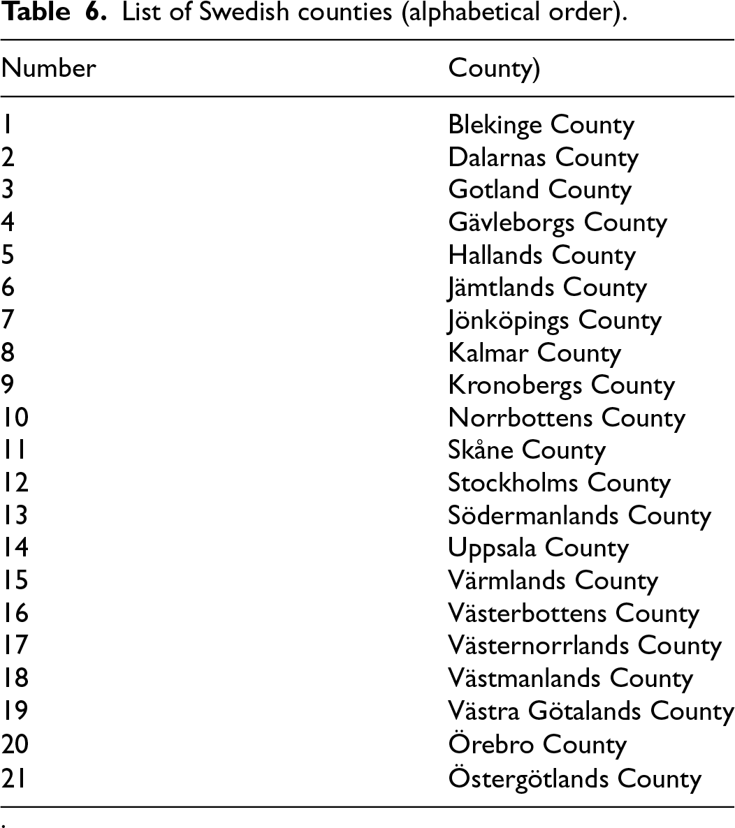
| Number | County) |
|---|---|
| 1 | Blekinge County |
| 2 | Dalarnas County |
| 3 | Gotland County |
| 4 | Gävleborgs County |
| 5 | Hallands County |
| 6 | Jämtlands County |
| 7 | Jönköpings County |
| 8 | Kalmar County |
| 9 | Kronobergs County |
| 10 | Norrbottens County |
| 11 | Skåne County |
| 12 | Stockholms County |
| 13 | Södermanlands County |
| 14 | Uppsala County |
| 15 | Värmlands County |
| 16 | Västerbottens County |
| 17 | Västernorrlands County |
| 18 | Västmanlands County |
| 19 | Västra Götalands County |
| 20 | Örebro County |
| 21 | Östergötlands County |
.