On loss compensation,amplification and lasing in metallic metamaterials

Abstract

The design of metamaterials, which are artificial materials that can offer unique electromagnetic properties, is based on the excitation of strong resonant modes. Unfortunately, material absorption—mainly due to their metallic parts—can damp their resonances and hinder their operation. Incorporating a gain material can balance these losses, but this must be performed properly, as a reduced or even eliminated absorption does not guarantee loss compensation. Here we examine the possible regimes of interaction of a gain material with a passive metamaterial and show that background amplification and loss compensation are two extreme opposites, both of which can lead to lasing.

Introduction

Metamaterials are designed, artificial materials enabling innovative properties that cannot be found in any naturally existing materials ^1,2 . Specifically, electromagnetic metamaterials are designed to provide tailored electromagnetic properties, for example, prescribed effective electric permittivity ε and magnetic permeability μ tensors. Consequently, they may offer full control over the propagation of electromagnetic waves inside the material. To achieve that, they are made from dense assemblies of subwavelength-size local artificial scatterers that are designed to exhibit a specific resonant response to electromagnetic radiation. In natural materials, this response originates from collective oscillations throughout the atoms of the crystal lattice. Borrowing this idea from the natural world, metamaterials are made of their own artificial meta-atoms, which are structural units properly designed and periodically arranged in a macroscopic lattice. ³ If the periodicity of this lattice is chosen much smaller than the operating wavelength, the overall structure behaves as an effectively homogeneous medium to an incoming wave, characterized by effective parameters ε _eff, μ _eff, irrespective of the subwavelength local spatial structure of the meta-atoms. In contrast to ordinary natural materials, metamaterials can be designed to exhibit frequency bands with simultaneously negative ε _eff and μ _eff in almost any desired frequency region—from radio frequencies to visible light. This can lead to various exotic effects, ^{4 –7} such as negative index of refraction (enabling flat lenses and superlensing), magnetic response with nonmagnetic materials and optical magnetism, zero reflectivity (useful to avoid reflection losses, e.g. for solar energy harvesting), zero index of refraction (for light concentrators, geometrical beam forming, etc.), to mention a few.

In practice, a resonant metamaterial is a driven oscillator system: The incoming wave collectively excites the meta-atoms, which in turn respond to the driving force with a secondary scattered wave. The metamaterial’s reflection is given by this scattered wave while the transmitted electromagnetic field results from the superposition of both. In order to achieve a negative effective permittivity ε _eff, permeability μ _eff, or even both simultaneously, the metamaterial unit cell must be properly designed to produce local resonant electric and/or magnetic moments that can couple to the corresponding fields of the incoming electromagnetic wave. Resonance is necessary to allow the response functions to become negative, that is, the driven electric or magnetic dipole moments to point opposite to the driving field over a certain frequency band. However, this is a necessary but not sufficient condition; the local metamaterial resonators or meta-atoms must be capable of storing enough electromagnetic energy to overcome the vacuum polarization. Mechanisms that damp the resonance or reduce the oscillator strength will cause a weak response and will probably prevent ε _eff and/or μ _eff to reach negative values. This, for example, may become a problem if we scale the operating frequency to the near infrared or visible region, ⁸ because dissipative losses in the metallic parts of the metamaterials can become very high and the resulting resonances broad and shallow. One obvious way of compensating for loss is to introduce gain materials into the metamaterial structure. ^{9 –26} This constitutes a promising solution, provided that we can achieve a sufficiently strong coupling between the gain material and the meta-atoms of the metamaterial, so that the resonance becomes loss compensated, that is, undamped.

Because metamaterials are designed to have a bulk response, they are homogenizable systems, that is, they can be replaced by a homogeneous system of the same effective response. In the presence of gain, though, the different ways of interaction between the gain and the local resonators may lead to qualitatively different systems, consequently raising nontrivial questions: Under which circumstances do the meta-atoms—which make up the metamaterial—predominantly interact with local gain to form new, undamped meta-atoms with sharpened resonant response, which subsequently homogenize into a new, loss compensated, bulk system? Or, in the opposite extreme, when do the meta-atoms homogenize to form a lossy bulk system that subsequently interacts with gain to produce an amplified output, without substantially reshaping the response function of the meta-atoms? In this article, we intend to put these questions in context, by examining the different coupling schemes between the metamaterial resonators and the gain system. We show that, depending on the level of coupling between the metamaterial and the gain material, different regimes are possible, such as loss compensation and amplification, both of which can lead to lasing. In order to understand how these regimes manifest in real experiments, we also demonstrate their distinct features in realistic pump–probe simulations.

Pump–probe experiments

In order to study the coupling of metamaterials with gain, the active material needs first to be excited (pumped), so that electrons are raised from the ground level to the upper level, and population inversion is achieved to provide the necessary gain (see Supplemental Material for details). Depending on the duration of the excitation, both transient and steady state effects can be examined, since with pulsed or continuous wave (CW) pump, time- or frequency-domain aspects can be examined, respectively. In real experiments, very high power short pulsed lasers allow for very high pump intensities and are usually more convenient than CW pumps. With such powerful lasers, the experiment becomes a time-domain problem and, as a consequence, the metamaterial with gain has to be probed with sufficiently short pulses in order to capture the dynamics. In essence, the study of the system becomes a pump–probe experiment. In such experiments, a short intensive Gaussian pulse (pump) of duration τ _pump is first sent to the system, in order to excite the gain material. After a certain time δτ _pp, the so-called pump–probe delay, and while the populations are returning to their ground state at a 1/τ _decay rate, a weak Gaussian pulse (probe) of duration τ _probe is sent through the system to capture its response under the effect of gain. Depending on the relative time scales between τ _decay, τ _pump, τ _probe and δτ _pp, this configuration can probe the dynamics at different regimes. For example, if τ _pump << τ _decay, then for different pump–probe delays δτ _pp, the probe pulse will monitor the system under decreasing gain, while at the opposite extreme where τ _pump >> τ _decay, the probe pulse will experience a quasi-CW pump regime of constant gain.

To understand a system’s response, it is crucial that one has access to quantities such as the fields, currents, populations, and so on. When simulating such complex nanophotonic systems, this is actually possible everywhere, even inside the materials. In real experiments, though, the access to all these quantities is limited and indirect measurements such as transmittance and reflectance are most of the times the only data available for interpretation. Especially when some gain material is present, the interpretation can sometimes be misleading, as an increase of the output power may reasonably imply amplification, but does not guarantee loss compensation. As it will be evident later, loss compensation is manifested as a spectral narrowing of the resonance (resonance undamping) and not necessarily increased output, that is, amplification. For instance, undamping the resonance may lead to increased impedance mismatch and therefore increased reflectance and reduced transmittance of the system. ^19,21

With pump–probe experiments, it is possible to acquire significant understanding of the underlying Physics, despite the limited access to all quantities of interest. Usually the transmittance, T, is the most convenient parameter to measure experimentally, mainly due to the minimum complexity required in appropriately aligning the optical components. Based on this information, a very useful and experimentally measurable quantity can be extracted, the differential transmittance ΔΤ/Τ, which is defined as the transmittance with pumping the active structure minus the same without pumping and dividing it by the total transmittance without pumping. ^12,19 The differential transmittance is actually an indicator of the level of coupling between the gain material and the metamaterial. For example, let us assume that the two systems are fully uncoupled (as can happen when they are placed arbitrarily far apart). In this case, the total transmittance T can be expressed as a product of the individual transmittances, T _MM and T _gain, for the metamaterial (MM) and the gain material, respectively, leading to

$\frac{\Delta T}{T}=\frac{T_{\text{MM}}{T}_{\text{gain}}^{\text{ON}}-T_{\text{MM}}{T}_{\text{gain}}^{\text{OFF}}}{T_{\text{MM}}{T}_{\text{gain}}^{\text{OFF}}}=\frac{T_{\text{gain}}^{\text{ON}}-T_{\text{gain}}^{\text{OFF}}}{T_{\text{gain}}^{\text{OFF}}}={\left(\frac{\Delta T}{T}\right)}_{\text{gain}}$

1

that is, ΔT/T of the combined system will be equal to ΔT/T of the bare gain (the superscript ‘ON/OFF’ indicates whether the gain material is pumped or not). If, on the other hand, the two systems are coupled, then the total transmittance cannot be considered as a product of T _MM and T _gain anymore and ΔΤ/Τ is expected to be different from that of the bare gain alone. In this example, in order to emphasize the effect of weak versus strong coupling, we have assumed for simplicity that the pump does not change the metamaterial transmittance T _MM. In the opposite case, this effect can be directly incorporated in equation (1), so that after a few calculations we may write $\Delta T/T=\left(T_{\text{MM}}^{\text{ON}}/T_{\text{MM}}^{\text{OFF}}\right)\times {\left(\Delta T/T\right)}_{\text{gain}}+\left(T_{\text{MM}}^{\text{ON}}/T_{\text{MM}}^{\text{OFF}}\right)-1$ , again expressing ΔT/T of the combined system in terms of ΔT/T of the bare gain explicitly. The qualitative effect of weak versus strong coupling exists regardless of whether or not the pump affects other material properties of the system. For instance, an ultrashort optical pump can significantly affect the conductivity of the metallic parts, leading to additional pump-dependent changes, ²⁶ whereas in an electrically pumped system (or in an optically pumped system with less intense but longer duration pump pulses), this effect would be absent. In any case, and regardless of the coupling level, the differential transmittance depends on the population difference ΔN (and therefore on the pump–probe delay δτ _pp), and since after excitation, the populations return to their ground state, ΔN tends to zero and similarly does ΔΤ/Τ, as shown in Figure 1. Because pumping the gain material leads to ΔΝ > 0 (i.e. population inversion), one would naturally expect that ΔΤ/Τ will be positive as well, as ΔΝ > 0 implies amplification and therefore an increased transmittance. Surprisingly, in a relevant experimental work, ¹² it was found that ΔΤ/Τ < 0 and the result was correctly attributed to loss compensation, as subsequently verified by simulations. ¹⁹ For the bare gain, on the other hand, it was found in both works ^12,19 that ΔΤ/Τ > 0, as expected.

Figure 1.

Schematic of a pump–probe experiment and definition of the differential transmittance. Top panel: The system is probed without any pump and T_pump ^OFF is measured (I _IN, I _OUT are the incident and transmitted intensities). Bottom panel: A pump pulse is sent, the system is probed with different pump–probe delays and T_pump ^ON is measured. ΔT/T = (T_pump ^ON − T_pump ^OFF)/T_pump ^OFF is then a function of the population inversion and, consequently, of the pump–probe delay (reproduced from Droulias et al. ³⁴ ).

Hierarchy of near-field interactions

The local resonators that comprise metamaterials are mainly coupled via their near-field. For relatively weak coupling, they form renormalized local resonators, that is, a new global resonator which bears the properties of a single unit cell oscillator, but with a renormalized response (due to the collective nature of the oscillation). For strong coupling, on the other hand, it is not unlikely that the resonators form an extended state, for example, a surface state. ^27,28

Regardless of the particular interaction strength between local resonators, because metamaterials are designed to have a bulk response, their properties should still homogenize under the interaction with the gain material. ²⁹ However, due to the presence of the new subsystem, the gain material, this does not necessarily happen in the same way as in the passive metamaterial anymore. The reason is that due to the presence of gain, new coupling channels appear as the gain material and the local resonators can be coupled via their near-field interaction, leading to two qualitatively different situations: (a) for weak coupling, the resonators can first homogenize and then couple to gain and (b) for strong coupling, the resonators can first couple to gain and then homogenize. The key difference between the two opposite possibilities has to do with whether the action of gain reshapes the spectral response of the metamaterial or not. For weak coupling (case (a)), the metamaterial has a homogenized response as if no gain was present, that is, the lossy resonances remain lossy. By switching the gain on, the metamaterial resonance does not change qualitatively and any nontrivial response is practically preserved, despite the lossy resonances. On the other hand, for strong coupling (case (b)), the two subsystems cannot be examined separately as previously and homogenization happens after the gain acts to change the oscillators, that is, to reshape their spectral response and undamp (sharpen) the resonances. This undamping of the resonance is what we refer to as loss compensation in this context.

Besides the near-fields, however, propagating (background) fields are also present because of the incoming waves, which are necessary to excite the metamaterial. Their presence is important, as they can excite the passive metamaterial and the active gain medium individually and effectively couple them, without the two systems being coupled to each other directly. In practice, while the near-field coupling can be eliminated (e.g. by placing the two systems far apart), the coupling via the plane waves is unavoidable and background amplification is therefore always present. This is manifested as an overall gain in weakly coupled systems (case (a)), but if the coupling between the resonance and the gain is much stronger than the coupling of each of them to the plane wave, then the resonance could eventually be favored and the metamaterial be loss-compensated. This is the case where either renormalized local resonators or extended states strongly couple to gain and then homogenize (case (b)). In the former case gain changes the local (renormalized) resonators which then form together a collective state, while in the latter case the local resonators form together a collective (extended) state which subsequently couples strongly to gain. In both possibilities, it is a collective state that homogenizes after the interaction with gain and, if the gain is removed from the vicinity of the resonant near-field, the weak coupling is restored and the gain mainly sees the propagating mode, favoring background amplification. All cases are summarized in Figure 2.

Figure 2.

Regimes of near-field coupling between metamaterial resonators (yellow) and gain (red) and the resulting homogenization limits. The orange slab in the middle represents the homogenized metamaterial, which can be derived from any of the four extreme cases shown. The metamaterial schematic shows 9 unit cells of typical SRRs. SRR: split-ring resonator.

Amplification versus loss compensation

To tune the near-field coupling between the passive metamaterial and the active material, there are several ways. The most obvious, probably, is to operate with a certain mode and change the separation between the two subsystems, ¹³ in order to tune the spatial overlap of the resonant mode with the gain. Alternatively, the gain-metamaterial separation can be left unchanged, as there is a significant degree of freedom in the selection of the actual resonant mode of the metamaterials. For the two extreme coupling regimes, let us consider two generalized examples. First, let us assume we want to minimize the coupling between the gain and the metamaterial. In this case, we desire that the metamaterial homogenizes first and then interacts with the gain to experience amplification. To do so, we have to make sure that the gain does not couple directly to the resonance (it couples inevitably via the averaged fields), which means that all resonant near-fields should be strongly localized and well separated from the gain. For a certain gain-metamaterial separation provided by, for example, some spacer, systems with quadrupole-like moments like cut-wire pairs or interleaved split-ring resonators (SRRs), ³⁰ should then homogenize more easily than single cut-wires or single SRRs, which have near-fields extending at much longer distances, due to their dipole-like moments. ^31,32 On the other hand, if we desire to achieve the exact opposite, that is, to couple the gain as tightly as possible to the near-field and as little as possible to the averaged field, we have to make sure that the gain material is driven almost exclusively by the near-field of the resonance, rather than the background. In this case, the gain could be placed only in the gaps of a single SRR (as examined in the study by Huang et al. ²¹ ) or in between the two layers of the interleaved SRRs, ³⁰ so that the ratio of the local field (which is dominated by the near-field of the resonance) to the universal background which is also driving the gain will be much more in favor of the resonance.

To demonstrate the general ideas described above, let us consider a metamaterial made of simple U-shaped SRRs. This is a system that has been studied extensively, as the SRR has served as the first and conceptually simplest magnetic meta-atom. ³ Figure 3(a) shows a single unit cell of the system considered, which is periodically repeated in the SRR plane to form a single layer. If desired, by placing several such layers periodically, a full three-dimensional metamaterial is possible. For the moment, no gain material has been incorporated and Figure 3(b) shows the calculated transmittance T, reflectance R, and absorptance A at normal incidence for a single layer of the passive structure shown in Figure 3(a). The metallic part is assumed to be silver of thickness 30 nm with its relative permittivity modeled by a Drude response: ε_{r, silver}(ω) = 1 − ω_p ² /(ω² +iωγ), with ω_p = 1.37 × 10¹⁶ rad/s and γ = 2.73 × 10¹³ rad/s. The dielectric substrate is assumed to have relative permittivity ε_{r, sub} = 9 and thickness 30 nm. This metamaterial is designed to have a resonant magnetic response at 200 THz (1.5 μm) and this resonant frequency can be identified as a dip in the transmittance. Because the incident electric field is polarized parallel to the gap, the magnetic resonance couples to the electric field, leading to an effective permittivity ε _eff, which is shown in Figure 3(c). ^33,34 For the retrieval of ε _eff, we have used our custom modified technique (see Supplemental Material), which has the advantage of conveniently lifting the branch selection ambiguity, once one proper branch has been identified. Our technique has been tested against other popular retrieval techniques ^35,36 and the results show excellent agreement.

Figure 3.

Passive SRR resonance (a) Schematic of one unit cell for the metallic SRR structure (yellow), placed on a thin dielectric (light blue) substrate. (b) Calculated transmittance T (black), reflectance R (red), and absorptance A (blue) for normal incidence, when the electric field polarization is parallel to the gap, in order to excite the magnetic resonance at 200 THz. (c) Retrieved effective permittivity ε _eff. SRR: split-ring resonator.

For simplicity, let us assume that our SRR system is suspended in air and let us now introduce a 20-nm thin gain layer at distance δz from the metamaterial, as shown in Figure 4(a). The gain material is embedded in a dielectric of host permittivity ε_{r, host} = 9 (same as the dielectric substrate) and the system is examined via self-consistent finite-difference time-domain calculations. Once it is pumped, this permittivity becomes dispersive according to the emission profile of the gain material, acquiring a negative imaginary part (accounting for gain) (see Supplemental Material for details on the four-level gain system and the simulations). To illustrate the basic ideas described in the previous section, we scan the gain-metamaterial separation δz under a constant homogeneous pump rate of R_p = 3 × 10⁸ s⁻¹ and monitor the resonance (we will later relate our findings with pulsed pump conditions).

Figure 4.

Distance-dependent coupling of gain with the SRR metamaterial for constant pump rate R_p = 3 × 10⁸ s⁻¹. (a) Schematic of gain layer (red) placed at distance δz away from the SRR substrate. (b) FWHM and (c) maximum of the real part of the retrieved effective sheet conductivity σ _eff with pump off (blue) and on (red) for different separations. After δz ∼ 60 nm the SRR becomes completely uncoupled from the gain material. SRR: split-ring resonator; FWHM: full width half maximum.

Modifications of the resonance under the action of gain can be identified either in the retrieved permittivity ε _eff of an equivalent homogeneous slab of finite (subwavelength) thickness or in terms of an effective conductivity σ _eff of an equivalent, infinitely thin, current sheet. The latter approach, in particular, avoids all periodicity effects which are inherent to the retrieval of the permittivity, ^37,38 as it does not involve the geometry of the effective system. To calculate σ _eff, we probe the current J oscillating in the metallic SRR ¹⁸ and then divide by the driving E-field at the same plane, so that the resonance is described by σ _eff ∼ J/E and changes due to gain can be identified in the full width half maximum (FWHM) and maximum of Re(σ _eff). As shown in Figure 4(b, c), for sufficiently large separations, the onset of gain does not induce any changes on the SRR resonance, indicating that the metamaterial is totally uncoupled from gain and the resonators may homogenize first and then couple to gain (case (a)). As the gain layer approaches the SRR, the evanescent near-field of the resonance starts overlapping with the gain region; the coupling between the two systems becomes stronger, which is observed as a reduced FWHM and an increased maximum of Re(σ _eff), indicating the undamping of the resonance. At this extreme, the resonators first couple to gain and then homogenize (case (b)). However, for our example, the considered pump rate is not enough to completely compensate loss, as such a case would be identified with Re(σ _eff) becoming a delta function.

Two extreme cases, for strong coupling (δz = 0) and absence of coupling (δz = 80 nm) are shown in detail in Figure 5, where their qualitative difference is evident in the retrieved sheet conductivities, σ _eff, shown in the top row; strong coupling causes a spectral narrowing of the resonance (Figure 5, top left panel), as opposed to weak coupling, which does not affect it (Figure 5, top right panel). The observed resonance shift from 200 THz (δz = 80 nm) to around 185 THz (δz = 0) is due to the change of the effective refractive index of the metamaterial’s surroundings, because of the displacement of the gain layer and has nothing to do with the coupling strength. While in the simulations σ _eff unambiguously indicates the coupling regime, in real experiments monitoring the currents is rather difficult and other quantities should be examined. For instance, looking at the absorptance A and the difference in absorptance between pump and no pump, ΔA, both systems show A > 0, that is, absorption despite the presence of gain, and ΔA < 0, indicating background amplification (Figure 5, middle row). Simply put, incoming waves experience less absorption once the pump is switched on and this is seen as amplification or ΔA < 0. Hence, observing just A or ΔA can be misleading, since only the strongly coupled configuration will correspond to loss compensation. Loss compensation is identified as a narrowing in ΔT/T around the resonance (bottom left panel of Figure 5), as also reported in previous works, ^12,13,19,21 and does not guarantee increased transmittance, contrary to what one might expect. The sign of ΔT/T indicates whether the transmittance is increased or not due to pump and, while here we find ΔT/T < 0 at the resonance, in the study by Huang et al. ²¹ we showed that, depending on the impedance mismatch between the system and the exterior, ΔT/T > 0 is possible as well. In all cases, due to reduced absorption, if the transmittance reduces, then the power excess should appear as an increased reflectance and vice versa. ^19,21 The actual sign, however, of ΔT/T does not convey any information on whether loss compensation is achieved or not.

Figure 5.

Strongly coupled for δz = 0 nm (left column) and fully uncoupled for δz = 80 nm (right column) SRR and gain for constant pump rate R_p = 3 × 10⁸ s⁻¹. Top row: Retrieved effective sheet conductivity σ _eff with pump off (blue) and on (red). Middle row: Absorptance A and difference in Absorptance ΔA. Bottom row: Transmittance T without pump (solid line) and Differential Transmittance ΔT/T where blue (orange) regions denote negative (positive) ΔT/T. Loss compensation is identified as a narrowing in ΔT/T around the resonance and happens only for the strongly coupled case (left column). SRR: split-ring resonator; FWHM: full width half maximum.

The homogenization regime can be also identified in the retrieved permittivity ε _eff of a thin slab. In Figure 6, ε _eff is shown for the two extreme cases presented in Figure 5. For the strong coupling case, similar conclusions are extracted, as the onset of gain clearly makes Im(ε _eff) narrower. The undamping makes Re(ε _eff) even more negative around the resonance, verifying the effect of loss compensation: the retrieved ε _eff behaves as if the metamaterial was made out of lower loss resonators. This narrowing leads to increased Im(ε _eff), which, contrary to intuitive thinking, does not necessarily mean increase of losses. An increase in Im(ε _eff) means that more power can be transferred from the input signal to the resonator. If the impedance mismatch with the exterior does not change or improves, this immediately translates into increased absorption of the incoming wave from the system. However, if this increase causes a larger impedance mismatch, less power can be absorbed by the system, despite having increased Im(ε _eff) and the overall response could appear as reduced absorption, as in our case (Figure 5, middle left panel). In the case of weak coupling, the observations on ε _eff differ from those on σ _eff, because the currents are normalized by the driving field (σ _eff ∼ J/E). This means that changes in the SRR current due to gain which induce changes in the scattered field do not appear in σ _eff, but do in ε _eff, as ε _eff is extracted from the scattered fields. As seen in Figure 6, with increasing gain, the resonance becomes shallower, because the gain (not originating from the near-field) just adds on the metamaterial loss, to produce a less positive Im(ε _eff) and a less negative Re(ε _eff) (exactly opposite of what is desired). This linear superposition ¹⁵ implies weak or absent coupling between the gain and the metamaterial and hence, this system lies fully in the background amplification regime; with increasing pump it becomes less absorbing (can even amplify the incoming wave with the appropriate amount of gain), while the resonance becomes shallower and shallower, until the negative Re(ε _eff) is lost.

Figure 6.

Retrieved effective permittivity ε _eff with pump off (blue) and on (red) with R_p = 3 × 10⁸ s⁻¹. SRR and gain strongly coupled for δz = 0 nm (left panel) and fully uncoupled for δz = 80 nm (right panel). In the right panel a pump of 3 × R_p has been used to emphasize the subtle effect.

Next, it would be useful to examine the same examples under pulsed pump conditions, as in typical pump–probe experiments. The major difference to the constant pump case is that the provided gain is not constant anymore; it decays asymptotically to zero once the pump pulse has excited the material and hence, the gain experienced by the probe depends on the pump–probe delay δτ _pp. Let us consider a realistic gain material, as is described in the Supplemental Material, with τ ₂₁ = 80 ps, τ ₃₂ = τ ₁₀ = 0.05 ps, and a probe pulse of duration τ _probe = 10 fs. Because for our considered material τ ₂₁ >> τ ₃₂, τ ₁₀, the gain relaxation time (called τ_decay in “Pump–probe experiments” section) is practically equal to τ ₂₁, which is much larger than the probe duration. Hence, despite the population relaxation, the probe practically experiences a constant population inversion (gain), the magnitude of which depends on the pump–probe delay δτ _pp. For example, for a Gaussian pump of the form $R_p\left(t\right)=R_{p0}\text{exp}\left[-{\left(t-t_0\right)}^2/{\tau }_{\text{pump}}^2\right]$ with τ _pump = 0.15 ps and R_{p 0} = 1 × 10¹¹ s⁻¹, it can be easily calculated from the rate equations (see Supplemental Material) that approximately 9 ps after the excitation time t ₀, the population inversion reaches the same level as for the constant pump of R_p = 3 × 10⁸ s⁻¹ which has been used so far. This means that for a pump–probe delay of δτ _pp = 9 ps, the results should be the same as in Figures 4 to 6. Indeed, simulations with these parameters fully reproduce the results shown so far, allowing us to use the CW conclusions as a general reference point. In practice, for a given gain material, the results obtained for different CW pump levels correspond to a family of (τ _pump, R_p0 , δτ _pp) parameters in pulsed pumped experiments, as long as the relative time scales allow (as in our case).

Nevertheless, it is interesting to see how the previous conclusions can be drawn in time-domain experiments. To relate the time-domain results with the previously presented CW pump results we use a Gaussian pump of τ _pump = 0.15 ps and R_{p 0} = 1 × 10¹¹ s⁻¹. As discussed, with this excitation results as those shown in Figure 5 (bottom row) are expected to be reproduced for δτ _pp = 9 ps, as for longer pump–probe delays the populations relax, leading to less gain and hence less pronounced effects. For the time-domain simulations we use a narrowband probe of 2 THz width (τ _probe = 0.2 ps) and change its center frequency in 2 THz intervals, to sweep a 10 THz range around the resonance of the system. For different pump–probe delays we probe the system and summarize the results for ΔT/T in Figure 7. The cases of strong coupling (δz = 0 nm) and absence of coupling (δz = 80 nm) are shown in the left and middle panel, respectively. For comparison, we also run the same experiment for the 20-nm thin bare gain film, which is assumed to have an emission peak at 200 THz and bandwidth of 20 THz. Note that for the composite system, the resonance is located at approximately 184 THz when δz = 0 nm and at approximately 199 THz when δz = 80 nm, as already observed in Figure 5. To enable easy comparison we avoid the mismatch between gain emission and the metamaterial response; throughout this article we tune the gain material to emit at each individual resonant frequency (for all previous and following results). The probe center frequency for each system is shown inside each panel. Clearly, the features of ΔT/T already discussed in Figure 5 for CW pump can be observed in the pulsed pump experiment as well for δτ _pp = 9 ps, as expected, which for larger pump–probe delays become less prominent, in accordance with the population relaxation. For the strongly coupled case, ΔT/T becomes negative at the resonance and changes sign as we move away. For the weakly coupled case and the bare gain ΔT/T remains positive around the resonance.

Figure 7.

Differential transmittance ΔT/T as obtained from time-domain numerical pump–probe experiments. Left: SRR and gain strongly coupled (δz = 0 nm). Middle: SRR and gain uncoupled (δz = 80 nm). Right: bare gain. The width of the probe signal is 2 THz and its center frequency, which is shown inside each panel, is swept around each resonance at intervals of 2 THz. SRR: split-ring resonator.

From amplification and loss compensation to lasing

The two cases studied so far (representing the two extreme coupling regimes) refer both to systems that support a resonant mode which, for adequate gain, can provide the necessary resonant feedback to make a laser. However, because they are entirely different in terms of how the gain interacts with the metamaterial, they serve as different laser resonators. The weakly coupled system does not differ much from ordinary lasers, where a gain material interacts with a homogeneous dielectric background (host). In our case, of course, the background is not a simple dielectric anymore, but a nanophotonic system having a complicated homogeneous (bulk) response. The metamaterial provides the necessary feedback to make lasing possible via the resonant mode into which stimulated emission takes place. On the other hand, the strongly coupled system takes this concept one step further; the resonance which is coming from the metamaterial provides the local field enhancement, to which the gain now can couple directly. Hence, the strong coupling can increase the interaction with the gain material and lead to lower lasing thresholds, just as band edges increase the interaction with gain in Photonic Crystal lasers. ^39,40

To study the transition to lasing, we excite the two systems with constant pump and scan a range of R_p = 10⁶ s⁻¹ − 10¹¹ s⁻¹. As expected, the lasing threshold for the strongly coupled system, which occurs at R_p = 9 × 10⁹ s⁻¹, is much lower than that of the weakly coupled system (R_p = 1.4 × 10¹⁰ s⁻¹). For comparison, we repeat the calculations in the absence of the metamaterial, that is, only when the 20-nm thin bare gain layer is present (with emission frequency at 200 THz), which starts to lase at an even higher pump rate, R_p = 3.5 × 10¹⁰ s⁻¹.

The results are shown in Figure 8, where the white horizontal dashed lines denote the resonant frequency of each system, which for the bare gain is just the emission frequency. The black vertical dotted lines correspond to the results for the cases shown in Figure 5. The shaded areas denote the lasing region for each system, where the system becomes a self-sustained oscillator and the output does not depend on the probe signal anymore. Hence, quantities such as transmittance and absorptance become meaningless and are not shown. As the pump increases, the strongly coupled system (left column) reaches full loss compensation for R_{p, comp} = 9.5 × 10⁸ s⁻¹, which is observed as a dramatic narrowing of Re(σ _eff). Note that this narrowing does not imply transition to lasing, because what is being monitored is an effective material property (σ _eff) and not the actual resonant mode (this will be discussed later in Figure 10). After this point the resonator changes character to become amplifying, fact that is observed in the sign reversal of max[Re(σ _eff)], as seen in the second row panel. The resonance starts to broaden with increasing pump, until the gain becomes enough to overcome the radiative loss as well and the system passes on to lasing. This resonance broadening that seems counter-intuitive at first glance, can be understood if we model the retrieved σ _eff as an effective material property with a Lorentzian response ∼ (ω ² – ω ₀ ² + iωγ) ⁻¹ . For no pump this response has γ > 0, but as the pump is increased, the loss is reduced and γ becomes less positive, until R_p = R_{p, comp}, where γ = 0 and the resonance becomes a delta function. For higher pump, γ changes sign and as the pump keeps increasing γ becomes more negative, that is, the resonance becomes broader. To examine the overall amplification, one has to observe A and ΔA. As seen in the third row of Figure 8, A can become negative (gain) regardless of the SRR resonance undamping (notice that A becomes negative in all three cases). As already discussed in Figure 5, ΔA < 0 for all three cases, indicating background amplification. On the other hand, ΔT/T shows a dramatic change only around the loss compensation pump rate (left column). For the uncoupled configuration (middle column) the resonance does not change at all as the pump increases (top two panels). Nevertheless, the increasing gain at some point overcomes the dissipative and radiation losses leading to lasing. In case of the bare gain (right column), gain has to overcome only radiative losses, but because there is no strong local mode to favor stimulated emission, gain has to be increased significantly in order to lase into some propagating mode.

Figure 8.

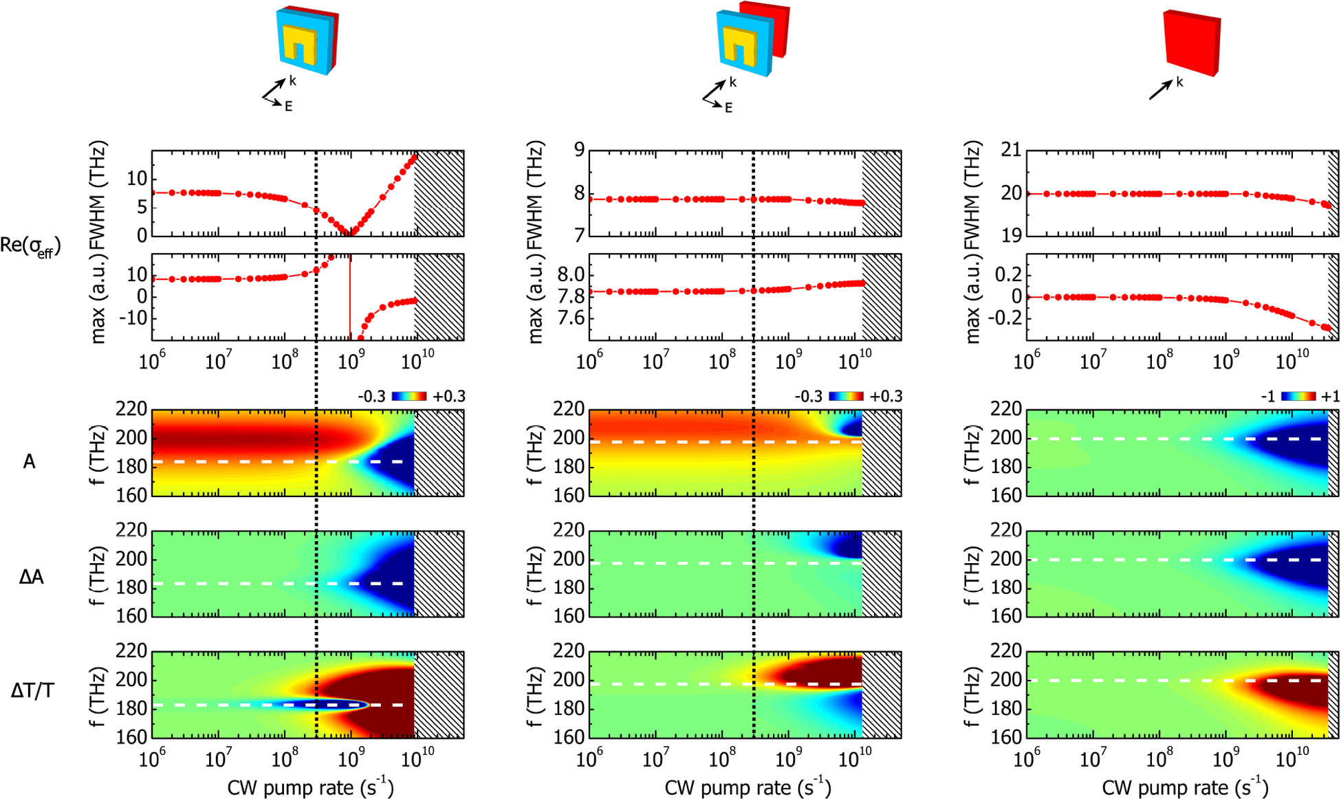
Pump-dependent behavior for SRR and gain when they are (a) strongly coupled (δz = 0 nm) and (b) uncoupled (δz = 80 nm). In (c) the case of bare gain is also shown for comparison. The horizontal white dashed line denotes the resonant frequency and the vertical black dotted lines indicate a cross-section corresponding to the results shown in Figure 5. The shaded area denotes that the system lases.

To demonstrate how stronger coupling can lead to even lower lasing thresholds, we exchange the position of substrate and gain, attaching the gain directly on the SRR and putting the substrate right below. This is the configuration previously examined in the study by Huang et al., ¹⁹ which has the same parameters as used in our examples here and a slightly thicker substrate of 40 nm. This has only the effect of reducing the resonant frequency further down to 175 THz, but has no other effect related to the lasing threshold. For these simulations we insert noise into the system and pump the electrons with a constant pump rate R_p . Then we monitor the emitted electric field away from the system in both polarizations, that is, parallel and perpendicular to the SRR gap. As can be seen in the lasing curves presented in Figure 9, the lasing threshold is now located at R_p = 1 × 10⁹ s⁻¹, almost an order of magnitude lower than our previously examined strongly coupled example. This is observed for the polarization parallel to the gap, indicating the involvement of the magnetic SRR mode in the lasing. For the other polarization, higher pump is needed to reach lasing, but this case is not further examined, as other modes which are beyond the scope of this analysis are probably involved. ³²

Figure 9.

Emitted power for varying pump rate for a system with gain layer attached on the SRR (simulated configuration as appears in the study by Huang et al. ¹⁹ ). E-field measured parallel to the gap (red connected dots) and perpendicular to the gap (blue connected dots). The passage to lasing at approximately 10⁹ s⁻¹ for the E-field parallel to the gap indicates the contribution of the SRR magnetic mode. SRR: split-ring resonator.

Observable regimes for different gain materials

The passage from loss compensation to lasing in a strongly coupled system presupposes that adequate gain is available. The maximum available gain depends on the maximum population inversion that can be achieved with a certain gain material, which in turn depends nonlinearly on the pump rate; as the pump increases, the population inversion at first increases linearly, until it enters a nonlinear region in which it saturates and further pump does not offer more gain. Our gain system was cautiously chosen to provide enough gain, almost entirely within the linear region, and the passing from loss compensation to lasing was made possible. In general, though, this does not have to be the case.

To illustrate how the available gain may limit the observable regimes, we change the total population of $N_{\text{total}}=N_{\text{total}}^{(0)}=5\times {10}^{23}$ and examine the FWHM of Re(σ _eff) as a function of the CW pump rate for our strongly coupled (δz = 0 nm) system. The results are shown in Figure 10. In the top panel of Figure 10 we also plot the population inversion ΔΝ for each examined case in order to facilitate the identification of the gain linearity. The horizontal black line denotes the necessary population inversion to reach lasing, ΔΝ _threshold, and the shaded area above denotes excess of gain. The vertical dotted lines denote the lasing threshold for each individual system. The resonant current J is the source of the coherent radiative output of the lasing state. For the proper amount of gain, the system passes on to lasing, that is, the resonant current J becomes spectrally a delta function as gain balances all dissipative and radiative losses, and the system becomes a self-sustained oscillator, radiating a single coherent mode. Hence, the passage to lasing is directly indicated as a spectral narrowing of the resonant current J, which is shown in the middle panel for all cases studied. The results for the original system that has been studied so far (left panel of Figure 8) are plotted as red connected dots and it is evident from the top panel of Figure 10 that this system practically lies entirely in the linear range. First, if we increase the available total population to $10\times N_{\text{total}}^{(0)}$ we push the system completely into the linear region (blue lines in all three panels). Next, if we reduce N _total we push the system into the nonlinear region. In particular, for $0.5\times N_{\text{total}}^{(0)}$ (green lines) we are still able to observe all regimes, but it is evident that Re(σ _eff) is deformed due to nonlinearity. For $0.15\times N_{\text{total}}^{(0)}$ (magenta lines) this deformation becomes more prominent and, because the maximum available ΔN becomes less than ΔΝ _threshold, we stop observing lasing. Last, for even lower total population of $0.06\times N_{\text{total}}^{(0)}$ (black lines) even loss compensation becomes impossible. The continuous lines have been calculated from the simulated data of the original system (red connected dots), by analytically transforming the population rates [see Supplemental Material]. To verify their validity, the analytical curves have been overlapped sparsely with simulated points (open dots), showing excellent agreement.

Figure 10.

Regimes of loss compensation, overcompensation and lasing for the strongly coupled to gain SRR (δz = 0 nm), as a function of the total population inversion, which controls both the available gain and the margin of linear response. Top panel: Population inversion. Middle panel: FWHM of SRR current, J. Bottom panel: FWHM of retrieved effective sheet conductivity, σ _eff. The connected solid red dots correspond to the gain material considered throughout this article, showing that the system is still in the linear regime as it passes to lasing. As the available gain becomes less, the observable range becomes narrower. SRR: split-ring resonator; FWHM: full width half maximum.

Conclusion

Although both weakly and strongly coupled systems can lead to lasing, they are qualitatively different lasers, as stronger coupling can lead to increased interaction of the gain material with the metamaterial and therefore to lower lasing thresholds. For enough available gain, a metamaterial that supports some resonant mode may pass on to lasing, but this does not guarantee whether loss compensation in the metamaterial resonators will happen during the transition. Given that the available gain is adequate, to achieve loss compensation depends on how well the metamaterial couples with the gain material. In the one extreme case where this coupling is strong, the resonance may really change and this will appear as a significant sharpening. The currents and the retrieved material parameters should then behave as if the metamaterial was originally made out of lower loss resonators. In the other extreme case where the coupling is weak or absent, background amplification can become prominent and any change in the dispersion will be either weak or absent. When the coupling is strong, not only does the dispersion change significantly (undamping of the resonance), but the energy that is transferred from the gain material to the metamaterial is much higher, as it follows a J·E ∼ |E|² law. This means that the stronger the coupling, the stronger the local field is in the gain region, and the more efficiently energy is extracted from the gain system. For weak coupling, less energy is extracted and the gain power density is in general smaller. Of course, from the one extreme to the other where either background amplification or loss compensation is dominant, there is a great range of possibilities that bear characteristics of both.

Supplemental material

Supplemental Material, NAX817947-supplementary - On loss compensation, amplification and lasing in metallic metamaterials

Supplemental Material, NAX817947-supplementary for On loss compensation, amplification and lasing in metallic metamaterials by Sotiris Droulias, Thomas Koschny, Maria Kafesaki, and Costas M Soukoulis in Nanomaterials and Nanotechnology

Supplemental material

Supplemental Material, NAX817947-supplementary - On loss compensation, amplification and lasing in metallic metamaterials

Supplemental Material, NAX817947-supplementary for On loss compensation, amplification and lasing in metallic metamaterials by Sotiris Droulias, Thomas Koschny, Maria Kafesaki, and Costas M Soukoulis in Nanomaterials and Nanotechnology