Sage Journals: Discover world-class research

Abstract

In the last decade, the adoption of technological tools in manufacturing industry, such as the use of the Internet of Things (IoT) and Machine Learning (ML), has led to the advent of the industry 4.0 (I4.0). In this scenario, intelligent devices can generate large volumes of data about industrial machinery and equipment that can be used to make maintenance more efficient. Prognostics and Health Management (PHM) is an emerging maintenance strategy that uses systems’ Condition Monitoring through IoT sensors installed on machinery to diagnose their faults or estimate their Remaining Useful Life (RUL). This study aims to conduct a Systematic Literature Review (SLR) on the use of ML techniques in the field of PHM of industrial mechanical systems and equipment. 50 studies resulted eligible for the above-mentioned SLR. Diagnostics and prognostics approach and the ML algorithm types used in the 50 analyzed papers have been analyzed together with the Key Performance Indicators (KPIs) used for their validation. From the analyses, it was found that Shallow Learning and Deep Learning (DL) algorithms are the most applied ones, while KPIs are used differently according to the type of task classification or regression. Moreover, results highlighted that many authors still use artificial datasets to test their algorithms, instead of datasets based on real data retrieved by their components. For the last type of datasets, this paper also introduces a schematic framework to standardize the step-by-step diagnostics and prognostics process carried out by the authors.

Keywords

Machine learning prognostic and health Management fault diagnosis fault prognosis remaining useful life key performance indicators systematic literature review

Introduction

Words like “Internet of Things” (IoT), “Cyber-Physical Systems” (CPS), “Internet of Services” (IoS), “Digital Twins” (DT), and “Machine Learning” (ML) have laid the foundations for the so-called Industry 4.0 (I4.0), which has prompted many companies to completely renew the concept of maintenance, improving productivity, preventing downtimes and reducing costs.^1,2

Among the different maintenance strategies, Prognostics and Health Management (PHM) represents one of the most innovative, perfectly fitting into the new I4.0 scenario; indeed it is based on systems’ Condition Monitoring (CM) through IoT sensors installed on machinery.³ PHM absolves the two important tasks related to diagnosis and prognosis to define their health state and avoid unexpected failures by preventing damages.⁴ Different parameters can be monitored in PHM according to the type of equipment, such as temperature, vibration, pressure, acoustic emission, force, tension, and others.⁵ Industrial Structures, Systems, or Components (SSCs) are considered to be in a normal state if these parameters remain above a predetermined threshold.⁶ Indeed, the evolution in time of these parameters can be used to monitor any deviation from normal operating conditions, which can help to determine the time the equipment is in good condition before it falls into a state of non-healthy condition. Therefore, PHM is mainly focused on both Fault Diagnosis (FD), when a failure state is present and there is the necessity to investigate the source of the anomaly, and Fault Prognosis (FP), when the necessity is to predict the future degradation until complete failure occurs;⁷ in such last case, often, the Remaining Useful Life (RUL) of SSCs is estimated. RUL is defined as the time length from the current time to the end of the useful life, that is, when the system condition reaches the failure threshold.⁸ The forecasting window plays a crucial role in prognosis because the objective is to provide an estimate of the future time-step when a certain event will occur.⁹ In recent years, several methods to evaluate RUL or FD have been proposed, such as model-based, data-driven, or mixing both of them. Model-based approaches rely on the knowledge of the inherent system failure mechanism to build a degradation mathematical model to describe the physical nature of the fault;¹⁰ on the other hand, data-driven techniques rely on collected data to extract knowledge about the health status of the monitored equipment. This task is particularly suitable to be performed by ML algorithms.¹¹ These algorithms range from conventional Shallow Learning (SL) techniques such as Artificial Neural Network (ANN), Support Vector Machine (SVM), Decision Tree (DTR), RF, to more recent techniques, such as DL algorithms.¹²

Machine learning is arising as one of the major approaches for PHM and RUL estimates. Machine learning is mainly used for solving two types of tasks, namely, “Classification” and “Regression”. Classification tasks have a finite number of output classes, while, in regression tasks, an infinite number of outputs are represented as real-valued data. By its nature, the FD is a classification problem. RUL prediction, instead, is often a regression problem, even if there are rare cases in which the RUL is treated as a classification problem.¹³

Regardless of the type of algorithm used or the type of task faced, an important step in using ML in PHM is being able to measure the performance of the algorithm. Therefore, it is necessary to define Key Performance Indicators (KPIs) to determine the accuracy of an algorithm and the associated methodology.

The study aims to conduct a Systematic Literature Review (SLR) on the use of ML techniques in the field of PHM of industrial mechanical systems and critical equipment. To the best of the authors’ knowledge, the problem presented in this paper has not been addressed previously. Thus, to fill this gap, the study investigates diagnostics and prognostics applied to the industrial SSCs, the kind of ML algorithms used and on the Key Performance Indicators (KPIs) for validating them.

The rest of this paper is outlined as follows: next section presents the methodology followed to conduct the research that led to the identification of the selected studies; then, the results will be analyzed and discussed by carrying out a bibliometric analysis and answering the aforementioned RQs; finally, the last section highlights the conclusions and future works.

Research methodology

To have an overview on the use of ML techniques in the field of PHM of industrial SSCs, an SLR¹⁴ similar to the ProKnow-C methodology¹⁵ was performed to answer the following Research Questions (RQs):

- RQ 1. What are the most used ML algorithms for PHM’s diagnostics and prognostics of industrial SSCs?

- RQ 2. What are the main performance metrics of ML algorithms adopted in PHM of industrial SSCs?

To answer the aforementioned questions, a literature search was performed on the Scopus database (www.scopus.com), which is often used as a unique database because it groups several types of journals covering different fields of science and, in addition, it provides exhaustive data for each document and complete information on the author(s) and their institution profiles.^16–19 The research string was run on January 10, 2023. Aiming to restrain the search field to the desired themes only, several combinations of keywords have been used for including all the possible papers related to the concepts of:

- PHM (i.e., “PdM” OR “predictive maintenance” OR “data-driven PdM” OR “prognostic”, OR “condition-based maintenance”);

- diagnostics and prognostics (i.e., “fault” OR “RUL”);

- ML (i.e., DL).

Each of these keywords was searched in the abstract, title or keywords (TITLE-ABS-KEY) of the documents, that is, at least one keyword for each of the 3 above-mentioned batches must be present either in the title, or in the abstract, or in the document keywords. This query provided a first set of 483 results; then, some Inclusion Criteria (IC) were considered:

- IC 1. Only papers in the final publication stage;

- IC 2. Only English language papers;

- IC 3. Only recent papers that were published between 2008 and 2023.

This first filtering returned 418 papers; to further limit this number of documents, a fourth IC was added to the others:

- IC 4. Only journal papers (other kinds of documents, such as books or conference papers were not considered).

Following this last IC, the database was restricted to 254 documents. The final search string is reported below:

TITLE-ABS-KEY ((Prognostic PRE/2 Management OR “PhM” OR “Data-driven PhM” OR “Predictive Maintenance” OR PdM OR “Data-driven PdM” OR “prognostic*” OR “condition-based maintenance” OR CBM) AND (“Machine Learning” OR “ML” OR “Deep Learning” OR “DL”) AND (fault OR failure OR “Remaining Useful Life” OR “RUL”)) AND PUBYEAR >2007 AND PUBYEAR <2024 AND (LIMIT-TO (PUBSTAGE, “final”)) AND (LIMIT-TO (DOCTYPE, “ar”)) AND (LIMIT-TO (LANGUAGE, “English”)).

At this point, three further steps, described below, were conducted to finally find the ultimate papers:

First, 31 documents were removed by simply reading the papers and journals titles, because they were not related to the industrial mechanical systems field (i.e., medical, railway, robotics, or chemical field);

Second, the remaining 223 abstracts were analyzed, discarding 148 documents because either they did not consider industrial mechanical applications, but aeronautical, aerospace, and chemical applications, or they did not consider applications to validate their ML algorithms at all; the remaining 75 documents went to the next analysis step, even if 24 of these 75 needed a more in-depth analysis because by simply reading the abstracts, it was impossible to determine neither if authors considered some kind of applications, nor if the applications were in theme with the interested industrial field;

Finally, a full paper analysis was conducted, which allowed excluding 25 documents because they consider neither ML algorithms (but statistical techniques), nor industrial mechanical applications. Therefore, 50 papers out of the 254 were considered eligible for the following analysis.

An overview of the whole search process is provided in Figure 1.

Figure 1.

Overview of the literature identification process.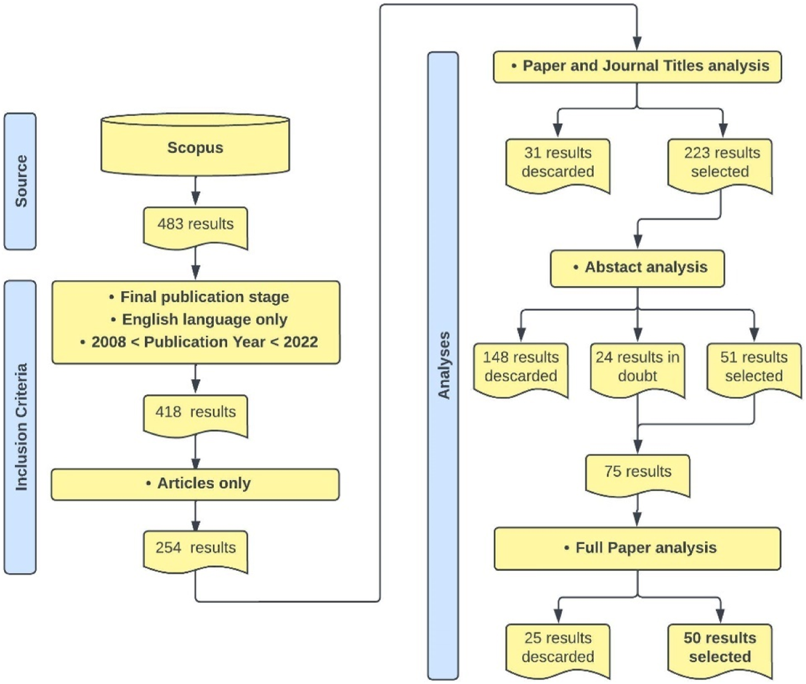

Results and discussion

In this section, the results are shown and discussed according to the previously defined RQs. First, in section 3.1, a bibliometric analysis²⁰ was carried out to highlight the trends of the analyzed publications over the years. Next, RQ 1 and RQ 2 were answered, respectively, in section 3.2 and section 3.3 where the ML algorithms and KPIs used in the 50 analyzed studies are examined; finally, in section 3.4, a schematic framework was developed to standardize the diagnostics and prognostics process carried out by the authors who used own unique datasets, and not the common public available datasets.

Bibliometric analysis

Figure 2 shows how the 50 selected papers are distributed over the years, including the number of citations received per year. They cover an 8-year long period, starting from 2016 until 2023, although the IC 3, defined in the previous section, considers eligible only papers starting from 2008. Only 20 papers of the first set of 483 results belong to the 2008–2015 years and none of them is about the industrial mechanical field, but medical, railway, chemical or aeronautical field. For such a reason, they were excluded from the final analysis. In Figure 2, it is possible to note that the number of papers increased in the last few years, reaching the peak of 14 publications in 2021. This increasing number of studies over the years is not surprising, considering that the word “Industry 4.0” was used for the first time in Germany in 2011, and precisely during the Hanover Fair, where the Communication Promoters Group of the Industry-Science Research Alliance (FU) announced a project for the development of the German industrial manufacturing sector, the “Zukunftsprojekt Industrie 4.0” ²¹; since then, the German model, combined to the improvements of the inter-connectivity of the IoT and robotics devices brought by Artificial Intelligence (AI) technologies, has inspired numerous researchers to continue researching the ML field to improve the productivity and reduce the costs related to industrial maintenance.²²

Figure 2.

Publication and citations trend per year.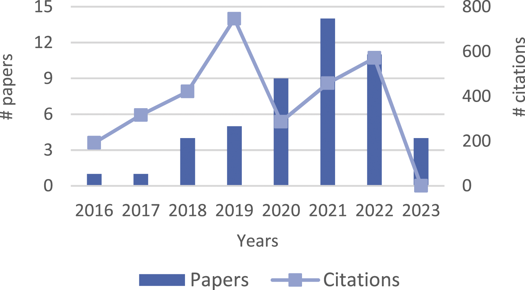

Concerning the number of citations per year, it is possible to note from Figure 2 that the trend is not stable, with a peak of 746 citations in 2019, an average of 373.8, and 0 citations in 2023, because of the narrow time window available to receive citations in this year, considering that the literature search date is on January 10^th, 2023.

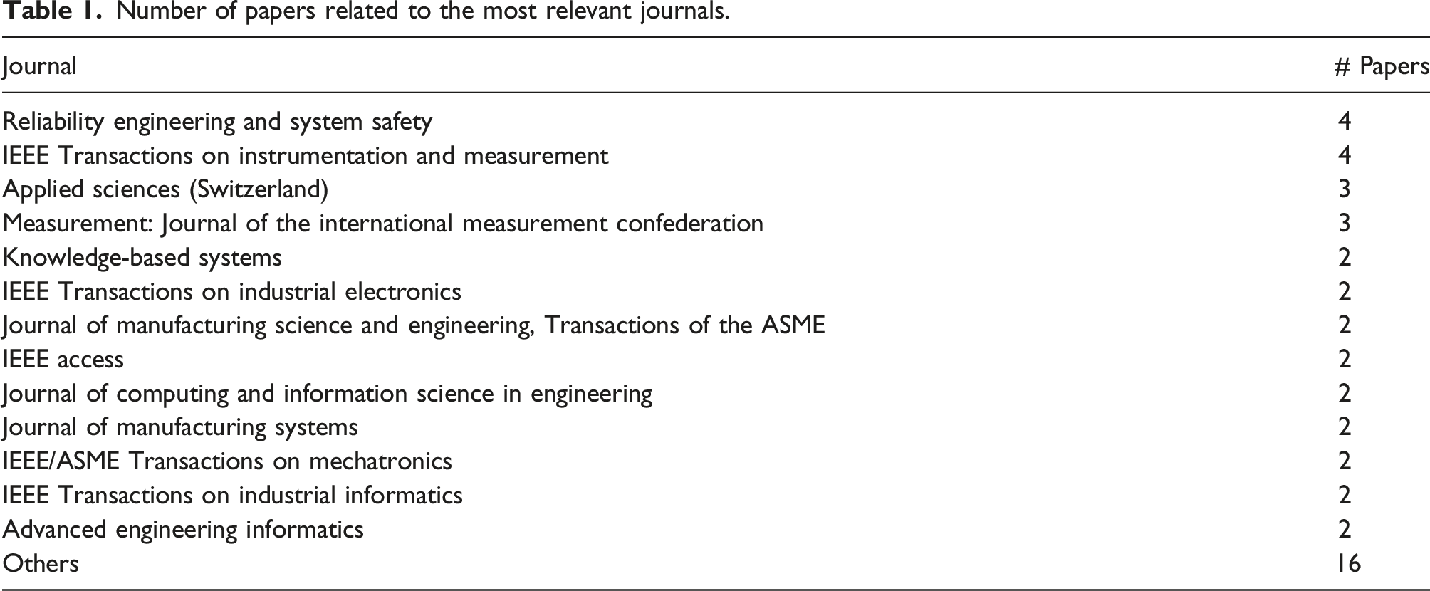
Table 1 shows the most relevant journals of the analyzed papers (journals with only one paper each were put together in the last row named “others”).

Table 1.

Number of papers related to the most relevant journals.

Journal	# Papers
Reliability engineering and system safety	4
IEEE Transactions on instrumentation and measurement	4
Applied sciences (Switzerland)	3
Measurement: Journal of the international measurement confederation	3
Knowledge-based systems	2
IEEE Transactions on industrial electronics	2
Journal of manufacturing science and engineering, Transactions of the ASME	2
IEEE access	2
Journal of computing and information science in engineering	2
Journal of manufacturing systems	2
IEEE/ASME Transactions on mechatronics	2
IEEE Transactions on industrial informatics	2
Advanced engineering informatics	2
Others	16

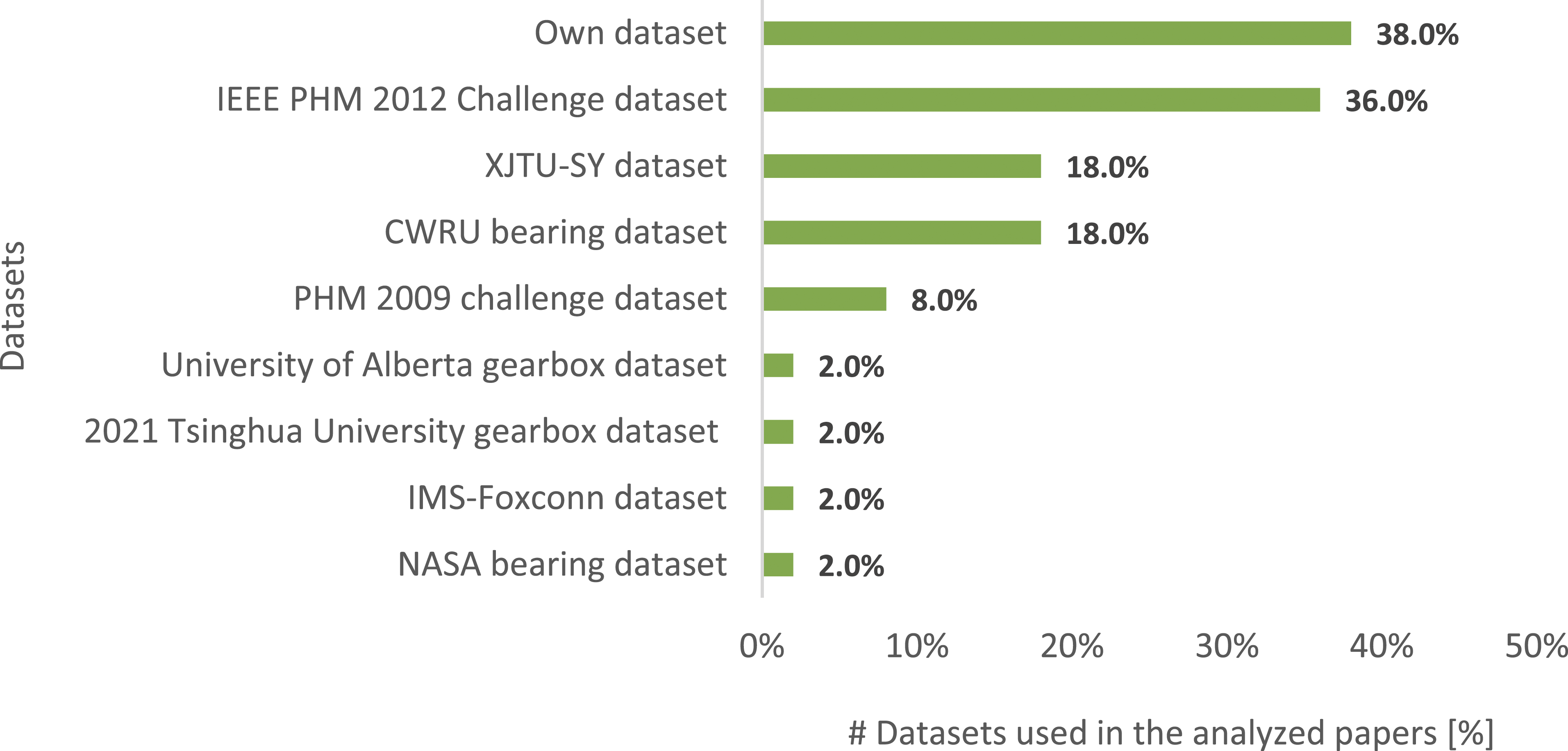
The 50 analyzed papers present 6 different types of SSCs (Figure 3) and 9 different types of datasets (Figure 4): 8 are online public datasets, and 1 is an “own-datasets” type, that is, datasets created specifically for the task addressed and the industrial application of the authors. It is possible to note that the sum of the percentage values in Figure 3 and in Figure 4 is beyond 100% because often more than one type of SSC and/or datasets was examined by the authors. About the mechanical systems and components analyzed in the papers, bearings are in 74% of the analyzed studies, followed by gears at 16%, milling machine’s cutting tools at 10%, a pump’s impeller, a ball screw and a hot strip mill’s roller at 2%. These trends can be explained by noting that the most of problems arising in rotating machinery are caused by faulty gears and bearings.²³ As components between the stationary and the rotating part of the industrial machinery, bearings represent an essential part of them; in fact, it causes more than 50% of induction motors’ failures mainly because of overheating, too high axial and radial loads, and electrical stress such as the presence of bearing currents.²⁴ As a consequence of the predominant presence of bearings and gears as SSCs analyzed by authors, four popular public datasets resulted to be the most used in the analyzed papers, that is, for bearings, IEEE PHM 2012 Challenge dataset (36%), XJTU-SY and CWRU bearing dataset at (18%), and, for gears, PHM 2009 challenge dataset at (8%). The remaining four datasets consist of two datasets for gearboxes (University of Alberta gearbox and 2021 Tsinghua University dataset), one dataset for milling machine’s cutting tools (IMS-Foxconn dataset), and one dataset for bearings (NASA bearing dataset). Moreover, from Figure 4, it is possible to note that 38% of the analyzed papers present datasets created for the specific problems investigated by the authors; this theme is examined in depth in section 3.4.

Figure 3.

Structures, systems, or components used in the analyzed papers.

Figure 4.

Datasets used in the analyzed papers.

Machine learning algorithms for PHM of SSCs

This section aims to respond to RQ 1, that is, What are the most used ML algorithms for PHM’s diagnostics and prognostics of industrial SSCs?

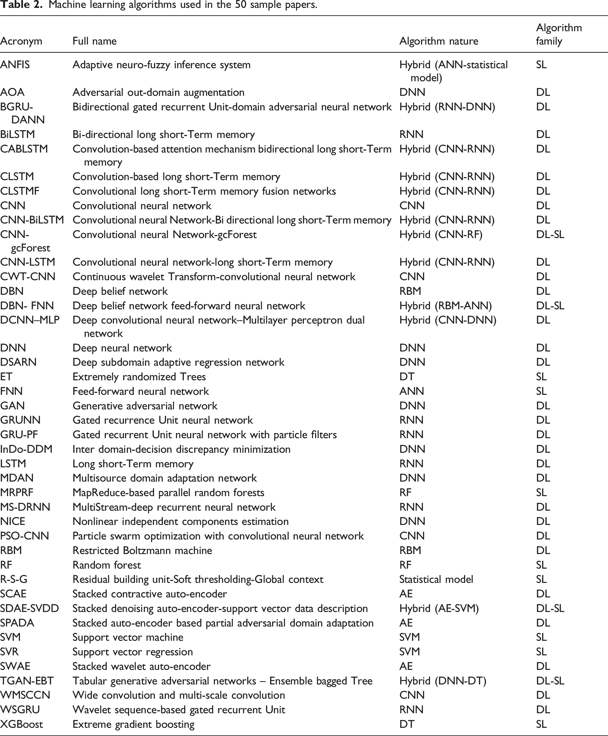
The constant increase in data availability due to intelligent sensors installed on SSCs, in addition to the technological progress in terms of computers’ hardware and software and a large number of cross-platform libraries, such as MATLAB, Python, R, and Sci-kit Learn, have led to the rapid development of multiple ML techniques to better address the issue of PHM of SSCs. These techniques range from the first classic SL techniques to the more recent DL ones. The word “shallow,” is from the single hidden layer belonging to the first simple neural networks, therefore usually nowadays “Shallow Learning” refers to all the traditional ML models, that is, those proposed before 2006;²⁵ among these, those used in the 50 analyzed studies are: shallow ANN, i.e., neural networks with only one hidden layer of nodes, SVM, DTR, RF, statistical models, and hybrids, that is, combinations of these algorithms; on the other hand, DL models are based on neural networks with the addition of multiple hidden layers between the network’s input and output;⁷ among these, those used in the 50 analyzed studies are: Deep Neural Network (DNN), Recurrent Neural Networks (RNN), Convolutional Neural Networks (CNN), Auto-Encoders (AE), Restricted Boltzmann Machines (RBM) and hybrids, that is, combinations of these algorithms. Furthermore, the cases of SL/DL hybrid methods, that is, algorithms in which SL and DL models are combined, are not uncommon.

Table 2 shows all the ML algorithms used in the analyzed papers, clarifying their nature (type of algorithm) and their family (SL, DL, or SL/DL hybrid methods).

Table 2.

Machine learning algorithms used in the 50 sample papers.

Acronym	Full name	Algorithm nature	Algorithm family
ANFIS	Adaptive neuro-fuzzy inference system	Hybrid (ANN-statistical model)	SL
AOA	Adversarial out-domain augmentation	DNN	DL
BGRU-DANN	Bidirectional gated recurrent Unit-domain adversarial neural network	Hybrid (RNN-DNN)	DL
BiLSTM	Bi-directional long short-Term memory	RNN	DL
CABLSTM	Convolution-based attention mechanism bidirectional long short-Term memory	Hybrid (CNN-RNN)	DL
CLSTM	Convolution-based long short-Term memory	Hybrid (CNN-RNN)	DL
CLSTMF	Convolutional long short-Term memory fusion networks	Hybrid (CNN-RNN)	DL
CNN	Convolutional neural network	CNN	DL
CNN-BiLSTM	Convolutional neural Network-Bi directional long short-Term memory	Hybrid (CNN-RNN)	DL
CNN-gcForest	Convolutional neural Network-gcForest	Hybrid (CNN-RF)	DL-SL
CNN-LSTM	Convolutional neural network-long short-Term memory	Hybrid (CNN-RNN)	DL
CWT-CNN	Continuous wavelet Transform-convolutional neural network	CNN	DL
DBN	Deep belief network	RBM	DL
DBN- FNN	Deep belief network feed-forward neural network	Hybrid (RBM-ANN)	DL-SL
DCNN–MLP	Deep convolutional neural network–Multilayer perceptron dual network	Hybrid (CNN-DNN)	DL
DNN	Deep neural network	DNN	DL
DSARN	Deep subdomain adaptive regression network	DNN	DL
ET	Extremely randomized Trees	DT	SL
FNN	Feed-forward neural network	ANN	SL
GAN	Generative adversarial network	DNN	DL
GRUNN	Gated recurrence Unit neural network	RNN	DL
GRU-PF	Gated recurrent Unit neural network with particle filters	RNN	DL
InDo-DDM	Inter domain-decision discrepancy minimization	DNN	DL
LSTM	Long short-Term memory	RNN	DL
MDAN	Multisource domain adaptation network	DNN	DL
MRPRF	MapReduce-based parallel random forests	RF	SL
MS-DRNN	MultiStream-deep recurrent neural network	RNN	DL
NICE	Nonlinear independent components estimation	DNN	DL
PSO-CNN	Particle swarm optimization with convolutional neural network	CNN	DL
RBM	Restricted Boltzmann machine	RBM	DL
RF	Random forest	RF	SL
R-S-G	Residual building unit-Soft thresholding-Global context	Statistical model	SL
SCAE	Stacked contractive auto-encoder	AE	DL
SDAE-SVDD	Stacked denoising auto-encoder-support vector data description	Hybrid (AE-SVM)	DL-SL
SPADA	Stacked auto-encoder based partial adversarial domain adaptation	AE	DL
SVM	Support vector machine	SVM	SL
SVR	Support vector regression	SVM	SL
SWAE	Stacked wavelet auto-encoder	AE	DL
TGAN-EBT	Tabular generative adversarial networks – Ensemble bagged Tree	Hybrid (DNN-DT)	DL-SL
WMSCCN	Wide convolution and multi-scale convolution	CNN	DL
WSGRU	Wavelet sequence-based gated recurrent Unit	RNN	DL
XGBoost	Extreme gradient boosting	DT	SL

Moreover, the frequency of citations of the aforementioned ML algorithms is shown in Figure 5, where it is clear the predominance of the DL methods (82%, i.e., 41/50 sample papers) both on the SL methods (10%, i.e., 5/50 sample papers) and Hybrid SL/DL ones (8%, i.e., 4/50 sample papers). One of the reasons for the higher use of DL, supplanting the traditional SL algorithms, is the ability to skip the process of hand-extraction features from the input data before being fed into the network, thanks to a nested series of consecutive computations that result in the extraction of a set of complex and highly informative features; moreover, in these years, an increasing number of empirical results have shown that these models return better results in terms of diagnostics and prognostics performance, compared to “shallow” methods. The main problem is that, compared with SL models, DL ones require a larger amount of training data (not always available) and the models to build are more complex.⁷

Figure 5.

Frequency of the shallow learning, deep learning, and hybrid algorithms used in the 50 analyzed papers.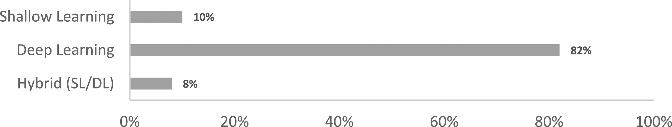

The pie charts in Figure 6 show how the ML techniques are distributed among the 50 sample papers, dividing them into SL algorithms (a), DP algorithms (b), and hybrid ones (c). About the SL algorithms, as aforementioned, only 5 of 50 analyzed papers use SL methods, with a prevalence of RF (30%, i.e., 3 times), followed by DT and SVM (20%, 2 times each), ANN, ANFIS (hybrid between ANN and a statistical model), and R-S-G statistical model (10%, 1 time each). RF, DT, SVM, and ANN have been used for prognostics tasks, while ANFIS and R-S-G statistical models for diagnostics tasks. About the DL algorithms used in 41 of the 50 analyzed papers, they are distributed as follows: CNN and RNN are the most used (25.6%, i.e., 11 times each), followed by DNN and Hybrid ones (16.3%, i.e., 7 times each) that are constituted by two models, that is, a mash-up between CNN and RNN (14%, i.e., 6 times) and a mash-up between RNN and DNN (2.3%, i.e., 1 time); the DL algorithms less used are RBM (9.3%, i.e., 4 times) and AE (7%, i.e., 3 times). CNN, DNN, RBM, AE, and Hybrid ones have been used both for prognostics and diagnostics tasks, while RNN has been used only for prognostics tasks. In conclusion, about the DL/SL hybrid algorithms, there are four of them: CNN-RF, RBM-ANN, DNN-DT, and AE-SVM; each of these algorithms has been used only for prognostics tasks.

Figure 6.

Types of shallow learning (a), Deep learning (b), and hybrid (c) algorithms used in the 50 analyzed papers.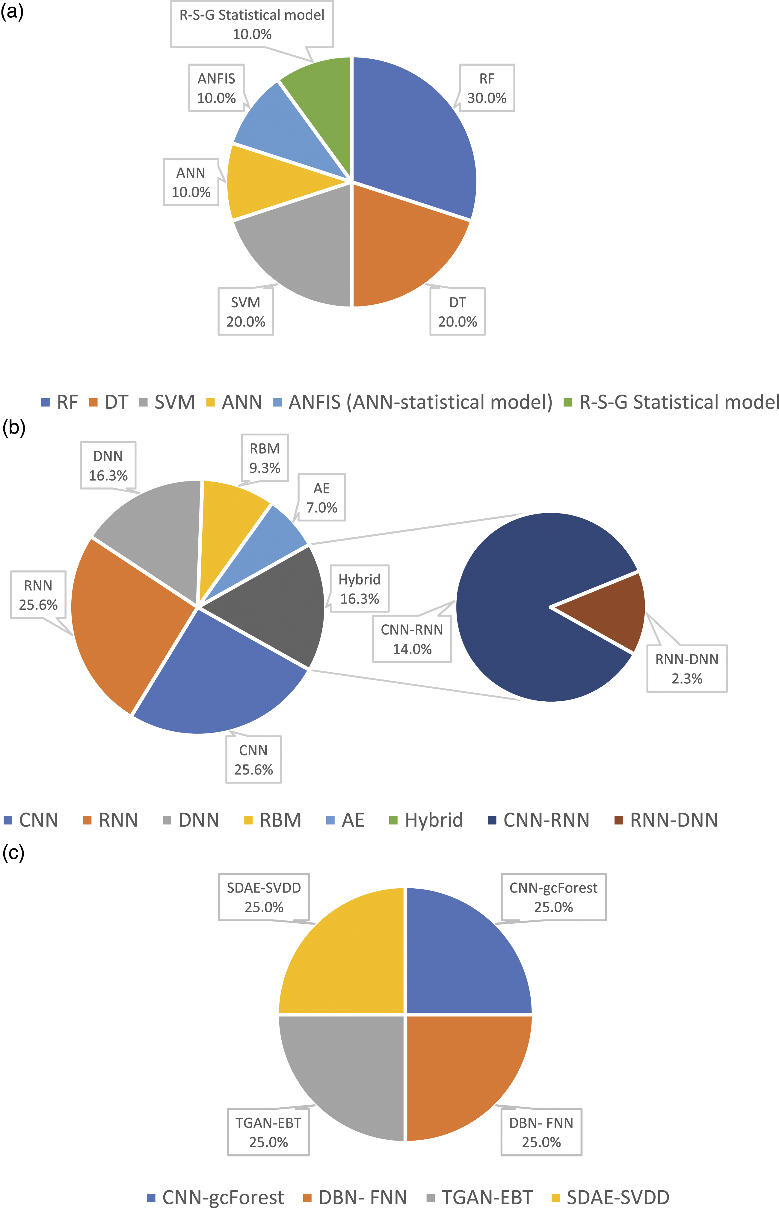

Machine learning KPIs for PHM of SSCs

The efficiency and effectiveness of an ML model can be evaluated using Key Performance Indicators. KPIs are usually divided into 2 groups: (i) KPIs for ML classification tasks, for which the output is divided by positive and negative classes. For instance, considering FD described through a simple binary classification, negative class stands for “fault” and positive class stands for “working”; (ii) KPIs for ML regression tasks, for which the output may be any value. For instance, for RUL, KPIs may range from 0 to 100, where 0 stands for “fault” and the other values stand for “still working.” Since different ML tasks produce different outputs (i.e., continuous or discrete), the related KPIs are consequently different too. To answer the RQ 2 (What are the main performance metrics of ML algorithms adopted in PHM of industrial SSCs?), first of all, a brief description of the Evaluation Metrics (EM) used in the 50 analyzed papers is shown in Table 3 (KPIs for classification tasks) and Table 4 (KPIs for regression tasks).²⁶

Table 3.

KPIs for ML classification tasks.

KPI	Formula	Description
Accuracy (A)	$A = \frac{T P + T N}{T P + T N + F P + F N}$ (1)	It is the ratio between the total number of correctly classified samples and the total number of samples within the test set. It is bounded to [0, 1], where 1 represents predicting all positive and negative samples correctly, and 0 represents predicting none of the positive or negative samples correctly.
Recall (R)	$R = \frac{T P}{T P + F N}$ (2)	It is the ratio between correctly classified positive samples and all samples assigned to the positive class. It is bounded to [0, 1], where 1 represents perfectly predicting the positive class, and 0 represents incorrect prediction of all positive class samples.
Precision (P)	$P = \frac{T C}{T C + F C} = {\begin{matrix} P P V = \frac{T P}{T P + F P} \\ N P V = \frac{T N}{T N + F N} \end{matrix}$ (3)	It is the ratio between correctly classified class samples and all samples assigned to that class. “Class” is a variable that can assume both “positive” (C = P) and “negative” (C = N) values. The positive case of the precision (C = P) is called “positive predictive value” (PPV) which is the ratio between correctly classified positive samples and all samples classified as positive, while the negative case of the precision (C = N) is called “negative predictive value” (NPV) which is the ratio between correctly classified negative samples and all samples classified as negative. P, PPV and NPV are bounded to [0, 1], where 1 represents all samples in the class correctly predicted, and 0 represents no correct predictions in that class.
F1 score (F1)	$F 1 = \frac{2}{1 / R + 1 / P}$ (4)	It is the harmonic mean of the R and the P; therefore, it penalizes extreme values of either. It is bounded to [0, 1], where 1 represents the perfect model (max R and P values) and 0 represents zero P and R values. Note that a high F1 value symbolizes a high P value as well as a high R value, while a low F1 value is not enough to know if the problem of the model resides on low Recall (type-I problem) or low Precision (type-II problem) or both of them (type-III problem). Therefore, F1 is often used together with other metrics, to better understand if the model suffers from the type-I, type-II, or type-III problem.
Area under the receiver operating characteristic Curve (AUROC)	$F P R = \frac{F P}{T N + F P}$ (5)	It is a curve plotted between false positive rate (FPR) on the x-axis and recall on the y-axis. FPR, just like recall, has values in the range [0, 1], but 1 represents incorrect prediction of all negative class samples, and 0 represents perfectly predicting the negative class. The AUROC value changes according to the model, but in the case of simple binary classification, the AUROC is equal to the equation (6). It is bounded to [0,1] where 0 means that the model is predicting a negative class as a positive class and vice versa, and 1 means that the model has a perfect capacity to separate the classes.
	$A U R O C = (T P + F N - \frac{T N (T P + 1)}{2}) / T N ∙ T P$ (6)
Confusion matrix (CMX)	$C o n f u s i o n M a t r i x = [\begin{array}{c} T P & F N \\ F P & T N \end{array}]$ (7)	It is a n_xn matrix, where “n” is the number of classes that are to be predicted. In the case of binary classification (n = 2), the confusion matrix looks like the equation (7). It is not exactly a performance metric but it is a starting point on which the other metrics, definable starting from the matrix, evaluate the results.

$T P$ = positive class samples correctly predicted; $T N$ = negative class samples correctly predicted; $F P$ = positive class samples incorrectly predicted; $F N$ = negative class samples incorrectly predicted; $T C$ = true class; $F C$ = false class.

Table 4.

KPIs for ML regression tasks.

KPI	Formula	Description
Mean squared error (MSE)	$M S E = \frac{1}{N} \cdot \sum_{i = 1}^{N} {(\hat{{R U L}_{i}} (t) - {R U L}_{i} (t))}^{2}$ (8)	It is the average of the squares of the errors, that is, the average squared difference between the predicted and the actual RUL values at i-th time-instant.
Root mean squared error (RMSE)	$R M S E = \sqrt{\frac{\sum_{i = 1}^{N} {(\hat{{R U L}_{i}} (t) - {R U L}_{i} (t))}^{2}}{N}}$ (9)	It is the root of the MSE and represents the standard deviation of the residuals (prediction errors); residuals are a measure of how far from the regression line data points are. The RMSE is more sensitive to outliers than the MSE because the effect of each error on RMSE is proportional to the size of the squared error.
Mean absolute error (MAE)	$M A E = \frac{1}{N} \cdot \sum_{i = 1}^{N} \| \hat{{R U L}_{i}} (t) - {R U L}_{i} (t) \|$ (10)	It is the arithmetic average between the predicted and the actual RUL values at time-instant t. MAE, just like MSE and RMSE, does not provide any “direction” of error, that is, whether the model is overfitting or underfitting the forecast. Moreover, it also measures the average magnitude of error, that is, how far the predictions are from the actual output.
Mean absolute percentage error (MAPE)	$M A P E = \frac{100 %}{N} \cdot \sum_{i = 1}^{N} \| \frac{\hat{{R U L}_{i}} (t) - {R U L}_{i} (t)}{{R U L}_{i} (t)} \|$ (11)	It is the arithmetic average between the predicted and the actual RUL values, related to the actual RUL values at time-instant t. It measures the forecast accuracy, evaluating the size of the error in percentage terms.
Coefficient of determination (R²)	$R^{2} = 1 - \frac{\sum_{i = 1}^{N} {({R U L}_{i} (t) - \hat{{R U L}_{i}} (t))}^{2}}{\sum_{i = 1}^{N} {({R U L}_{i} (t) - \bar{R U L})}^{2}}$ (12)	It is the proportionate amount of variation in the dependent variable explained by the independent variables in the linear regression model. It allows to understand how strong is the predictive capacity of a linear regression model.
Cumulative relative accuracy (CRA)	$C R A (λ) = \frac{1}{N} \sum_{i = 1}^{N} (w_{i} \cdot {R A}_{λ})$ (13)	It is a normalized weighted sum of relative accuracies at specific time instances (RA_λ). The latter is defined as a measure of the error in RUL prediction, relative to the actual RUL at a specific time index (RUL_i(λ_i)). RA_λ is used as a metric to emphasize that errors closer to the actual failure of a component are more severe. λ_i is defined as the normalized time and it is the ratio between the time-instant (t_i), and the time-to-failure of component (t_f); λ is bounded to [0,1], where 0 means that the component is on its maximum state of health, while 1 means that the component has failed.^27,28
Cumulative relative accuracy (CRA)	Where: ${\begin{matrix} {R A}_{λ} = 1 - \frac{\| {R U L}_{i} (λ_{i}) - \hat{{R U L}_{i}} (λ_{i}) \|}{{R U L}_{i} (λ_{i})} \\ λ_{i} = \frac{t_{i}}{t_{f}} \end{matrix}$
Scoring function (A_i)	$A_{i} = {\begin{matrix} \exp (- \ln (0.5) \cdot ({E r}_{i} / 5)) i f {E r}_{i} \leq 0 \\ \exp (\ln (0.5) \cdot ({E r}_{i} / 20)) i f {E r}_{i} > 0 \end{matrix}$ (14)	This metric was used for the IEEE PHM 2012 prognostic challenge, and it sets asymmetric penalties for late and early predictions. The letter “i” stands for i-th bearing, in fact, if there is more than one test bearing (as it often happens), it is possible to evaluate the average score of the RUL prediction for all testing bearings (A-score). A_i is 1 when the per cent error Er_i is 0; as the per cent error increases, the score decreases.²⁹
	$A - s c o r e = \frac{1}{N} \cdot \sum_{i = 1}^{N} A_{i}$ (15)
	Where: ${E r}_{i} = 100 % \cdot \frac{{R U L}_{i} (t) - \hat{{R U L}_{i}} (t)}{{R U L}_{i} (t)}$

$N$ = Cardinality of the dataset; ${R U L}_{i} (t)$ = i-th actual RUL value at t-instant; $\hat{{R U L}_{i}} (t)$ = i-th predicted RUL value at t-instant; $\bar{R U L}$ = mean value of the actual RUL samples in the dataset; ${R U L}_{i} (λ_{i})$ = i-th actual RUL value at λ-instant; $\hat{{R U L}_{i}} (λ_{i})$ = i-th predicted RUL value at λ-instant; $t_{i}$ = i-th time-instant; $t_{f}$ = time-to-failure of component; $w_{i}$ = i-th weight factor as a function of RUL at all time instants, that is, wi(RULi); ${E r}_{i}$ = percentage error of the i-th bearing.

Note: MSE, RMSE, MAE, and CRA are bounded to [0, +∞], while MAPE, R², and A_i are bounded to [0, 1]; since MSE, RMSE, MAE, and MAPE are coefficients that evaluate an error, the lower the value, the greater the accuracy of the forecast. Instead, for R², CRA, and A_i, the higher the metric, the better the prediction performance.

Moreover, the frequency of citations of the aforementioned EM is shown in the diagram in Figure 7, where the KPIs are divided into classification (a) and regression (b) tasks. Among all the 50 analyzed papers, 18 deal with the classification task, while the remaining 36 deal with the regression task. 4 papers considered both classification and regression tasks. About the classification task, Accuracy is the most used metric (58.6%, i.e., 17 times), followed by CMX (about 24.1%, i.e., 7 times), Recall (about 6.9%, i.e., 2 times), and AUROC, Precision, and F1 (about 3.4%, i.e., 1 time each). About the regression task, RMSE is the most used metric (32.4%, i.e., 22 times), followed by MAE (26.5%, i.e., 18 times), A_i (13.2%, i.e., 9 times), MAPE (11.8%, i.e., 8 times), R² and MSE (7.4%, i.e., 5 times each), and CRA (1.5%, i.e., 1 time).

Figure 7.

Frequency of the key performance indicators for classification (a) and regression (b) tasks.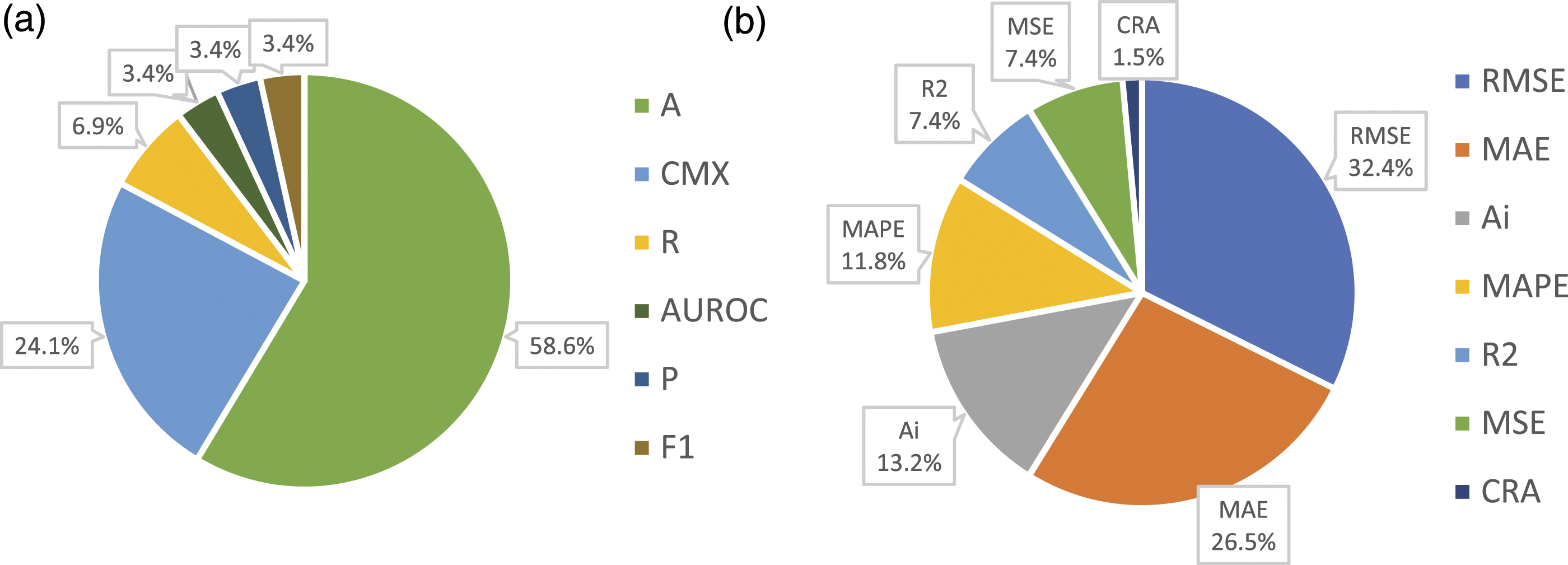

Table 5 below summarizes the main characteristics of the selected papers sorted by industrial application type, in terms of article, received citations, objective, industrial application(s), dataset(s), ML technique(s), ML task types, and KPI(s) used.

Table 5.

Characteristics of the selected studies.

Article	Cited by	Industrial application(s)	Objective	Dataset(s)	ML Technique(s)	ML task	KPI(s)
³⁰	27	Ball screw	Prognostics	Own dataset	GRU-PF	Regression	RMSE, MAE
³¹	46	Bearing	Diagnostics	Own dataset	DBN	Classification	A
³²	94	Bearing	Diagnostics	Own dataset;	CNN	Classification	A
³²	94	Bearing	Diagnostics	CWRU bearing dataset	CNN	Classification	A
³³	22	Bearing	Diagnostics	Own dataset	CNN	Classification	A
³⁴	16	Bearing	Diagnostics	CWRU bearing dataset	WMSCCN	Classification	A
³⁵	10	Bearing	Diagnostics	CWRU bearing dataset	NICE	Classification	AUROC
³⁵	10	Bearing	Diagnostics	XJTU-SY dataset	NICE	Classification	AUROC
³⁶	4	Bearing	Diagnostics	CWRU bearing dataset	CNN	Classification	A, (CMX)
³⁷	9	Bearing	Diagnostics	CWRU bearing dataset	R-S-G	Classification	A, P, R, F1, (CMX)
³⁸	0	Bearing	Diagnostics	CWRU bearing dataset	CNN-BiLSTM	Classification	A, (CMX)
³⁹	0	Bearing	Diagnostics	CWRU bearing dataset	CNN	Classification	A
⁴⁰	192	Bearing	Prognostics	IEEE PHM 2012 challenge dataset	RBM	Regression	A_i
⁴¹	100	Bearing	Prognostics	IEEE PHM 2012 challenge dataset	CWT-CNN	Regression	A_i
⁴²	264	Bearing	Prognostics	IEEE PHM 2012 challenge dataset	DNN	Regression	MAE, MAPE, RMSE
⁴³	175	Bearing	Prognostics	Own dataset	CNN	Regression	RMSE, CRA
⁴⁴	11	Bearing	Prognostics	IEEE PHM 2012 challenge dataset	MS-DRNN	Regression	MSE, MAE
⁴⁵	7	Bearing	Prognostics	IEEE PHM 2012 challenge dataset	LSTM	Regression	A_i
⁴⁶	52	Bearing	Prognostics	IEEE PHM 2012 challenge dataset	SDAE-T-GSVDD	Classification	A
⁴⁷	65	Bearing	Prognostics	IEEE PHM 2012 challenge dataset	GAN	Regression	RMSE, MAE, MAPE
⁴⁷	65	Bearing	Prognostics	XJTU-SY dataset	GAN	Regression	RMSE, MAE, MAPE
⁴⁸	15	Bearing	Prognostics	NASA bearing dataset	LSTM	Regression	RMSE, MAE, MAPE
⁴⁹	25	Bearing	Prognostics	IEEE PHM 2012 challenge dataset	DSARN	Regression	RMSE, MAE, A_i
⁴⁹	25	Bearing	Prognostics	XJTU-SY dataset	DSARN	Regression	RMSE, MAE, A_i
⁵⁰	12	Bearing	Prognostics	IEEE PHM 2012 challenge dataset	SCAE	Regression	RMSE, MAPE
⁵¹	82	Bearing	Prognostics	CWRU bearing dataset	CNN-gcForest	Classification	A, (CMX)
⁵¹	82	Bearing	Prognostics	XJTU-SY dataset	CNN-gcForest	Classification	A, (CMX)
⁵²	108	Bearing	Prognostics	Own dataset	CLSTM	Regression	RMSE, MAE
⁵³	18	Bearing	Prognostics	IEEE PHM 2012 challenge dataset	ET, RF, XGBoost, SVM	Regression	R², A_i
⁵⁴	11	Bearing	Prognostics	Own dataset	DBN	Regression	RMSE, MAPE
⁵⁵	7	Bearing	Prognostics	Own dataset	WSGRU	Regression	RMSE, MAE
⁵⁶	4	Bearing	Prognostics	IEEE PHM 2012 challenge dataset	BGRU-DANN	Regression	R², MAE, MSE
⁵⁷	39	Bearing	Prognostics	PHM 2012 challenge dataset	DCNN–MLP	Regression	RMSE, MAE
⁵⁷	39	Bearing	Prognostics	XJTU-SY dataset	DCNN–MLP	Regression	RMSE, MAE
⁵⁸	19	Bearing	Prognostics	IEEE PHM 2012 challenge dataset	CABLSTM	Regression	MAE, MSE, A_i
⁵⁹	8	Bearing	Prognostics	IEEE PHM 2012 challenge dataset	TGAN-EBT	Regression	RMSE, MAE
⁶⁰	3	Bearing	Prognostics	IEEE PHM 2012 challenge dataset	LSTM	Regression	RMSE, A_i
⁶¹	4	Bearing	Prognostics	IEEE PHM 2012 challenge dataset	CLSTMF	Regression	RMSE, MAPE
⁶¹	4	Bearing	Prognostics	XJTU-SY dataset	CLSTMF	Regression	RMSE, MAPE
⁶²	4	Bearing	Prognostics	IEEE PHM 2012 challenge dataset	MDAN	Regression	RMSE, A_i
⁶²	4	Bearing	Prognostics	XJTU-SY dataset	MDAN	Regression	RMSE, A_i
⁶³	0	Bearing	Prognostics	IEEE PHM 2012 challenge dataset	LSTM	Regression	RMSE, MAPE
⁶³	0	Bearing	Prognostics	XJTU-SY dataset	LSTM	Regression	RMSE, MAPE
⁶⁴	0	Bearing	Prognostics	Own dataset	GRUNN	Regression	MAE, RMSE
⁶⁵	0	Bearing	Prognostics	IEEE PHM 2012 challenge dataset	AOA	Regression	RMSE, MAE, A_i
⁶⁵	0	Bearing	Prognostics	XJTU-SY dataset	AOA	Regression	RMSE, MAE, A_i
⁶⁶	50	Bearing	Diagnostics	Own dataset	ANFIS	Classification	A
⁶⁶	50	Gear	Diagnostics	Own dataset	ANFIS	Classification	A
⁶⁷	14	Bearing	Diagnostics	Own dataset	PSO-CNN	Classification	A, (CMX)
⁶⁷	14	Impeller	Diagnostics	Own dataset	PSO-CNN	Classification	A, (CMX)
⁶⁸	22	Bearing	Diagnostics	CWRU bearing dataset	SPADA	Classification	A, (CMX)
⁶⁸	22	Gear	Diagnostics	PHM 2009 challenge dataset	SPADA	Classification	A, (CMX)
⁶⁹	0	Bearing	Diagnostics	CWRU bearing dataset	InDo-DDM	Classification	A
⁶⁹	0	Gear	Diagnostics	PHM 2009 challenge dataset	InDo-DDM	Classification	A
⁷⁰	86	Gear	Diagnostics	Own dataset	SWAE	Classification	A
⁷¹	1	Gear	Diagnostics	PHM 2009 challenge dataset	CNN	Classification	A
				2021 Tsinghua University gearbox dataset
				University of Alberta gearbox dataset⁷²
¹⁰	238	Gear	Prognostics	Own dataset	DBN- FNN	Regression	MAPE, RMSE
⁷³	163	Gear	Prognostics	PHM 2009 challenge dataset and own dataset	CNN	Classification	A, R, (CMX)
⁷⁴	20	Hot strip mill’s roller	Prognostics	Own dataset	LSTM, CNN, DBN	Regression	RMSE, MAE
⁷⁵	316	Milling machine’s cutting tool	Prognostics	Own dataset	FNN, RF, SVR	Regression	R², MSE
⁷⁶	37	Milling machine’s cutting tool	Prognostics	Own dataset	MRPRF	Regression	R², MSE
⁷⁷	40	Milling Machine’s cutting tool	Prognostics	Own dataset	BiLSTM	Regression	RMSE, MAE
⁷⁸	31	Milling Machine’s cutting tool	Prognostics	IMS-Foxconn dataset	BiLSTM	Regression	MAE
⁷⁹	8	Milling Machine’s cutting tool	Prognostics	Own dataset	CNN-LSTM	Regression	RMSE, MAE, R²

PHM framework for the “own-dataset papers”

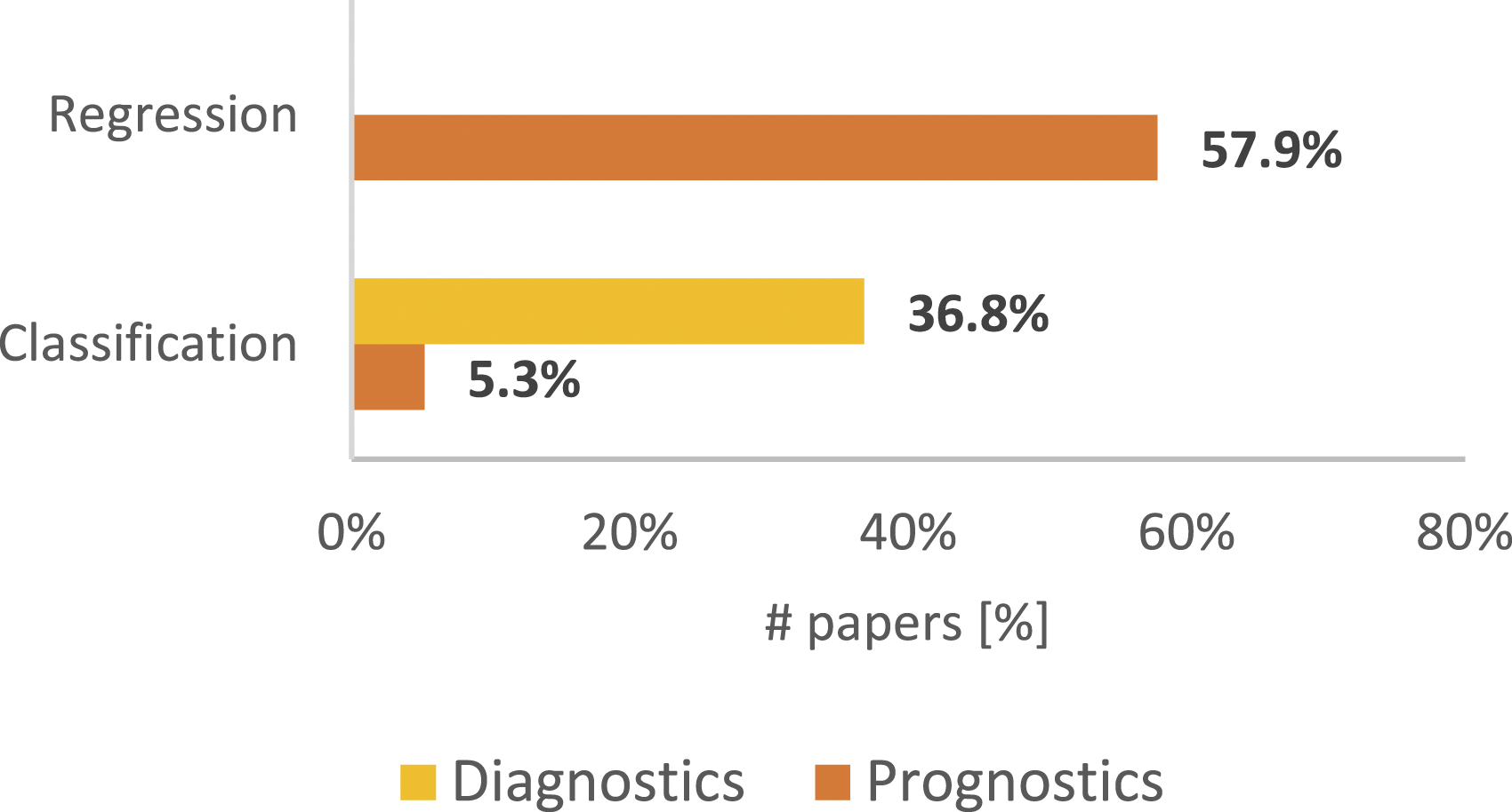
Figure 8 shows the analyzed papers’ diagnostics and prognostics distribution and how regression and classification tasks are allocated to them. It is possible to note that Prognostics overtakes its counterpart with 70% of the papers (divided by classification end regression tasks) versus 30% of the papers which face diagnostics (only through classification task). However, prognostics and diagnostics percentages, shown in Figure 8, could be misleading because they are not necessarily related to the real manufacturing industry prognostics and diagnostics data, but rather they are related to the problem of the complexity of monitoring and analyzing data through IoT devices for industries, that led to the use of pre-existing datasets just to find the best ML algorithms proposed by the 50 papers’ authors. This is the reason why the papers that present datasets created specifically for the task addressed by their authors (own-dataset papers) are further investigated in this section; from Table 5 it is possible to extrapolate that an own-dataset has been used in 19 of the 50 analyzed studies. As a first step, to better understand the real partition between prognostics and diagnostics in the industrial field, Figure 9 shows the own-dataset papers’ diagnostics and prognostics distribution related to regression and classification ML tasks. Comparing Figures 8 and 9, it emerges that both the prognostics and the diagnostics trends are confirmed, that is, a clear predominance both of Prognostics on Diagnostics and Regression on Classification.

Figure 8.

All papers’ diagnostics and prognostics distribution related to regression and classification Machine Learning (ML) tasks.

Figure 9.

Own-dataset papers’ diagnostics and prognostics distribution related to regression and classification ML tasks.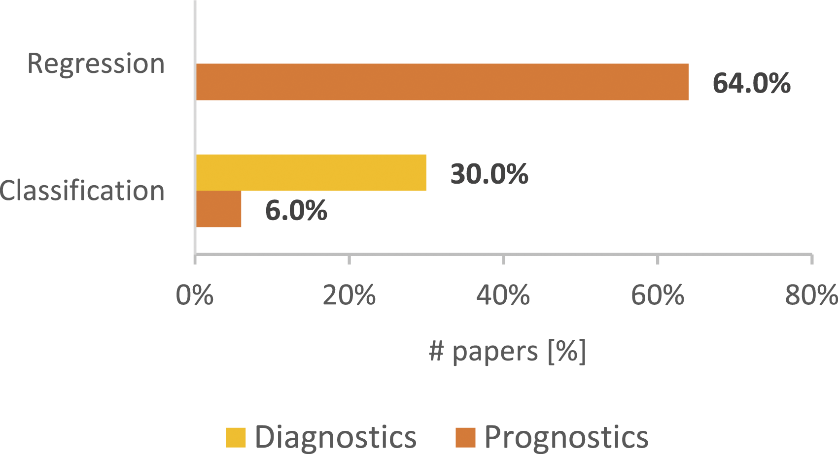

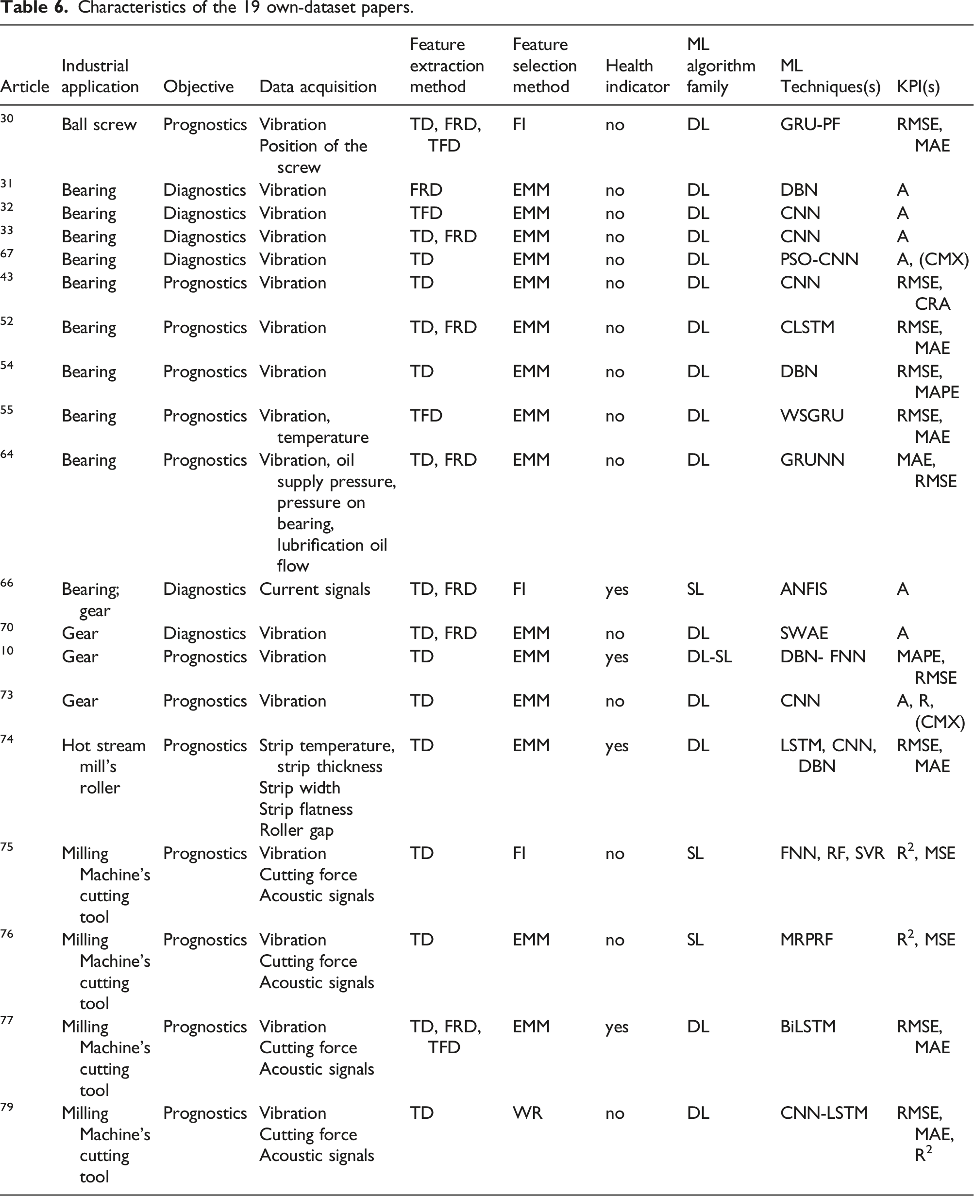
Therefore, Figure 10 below shows a single common PHM framework which describes the step-by-step diagnostics and prognostics process carried out by the authors of the 19 own-dataset papers. It is worth noting that the path is not unique since some steps could be repeated for the diagnostic and prognostic tasks, for example, although the prognostic step relies on the results of the diagnostic step, it may be necessary to perform steps from 2 to 5 again since the task purpose is changed. Moreover, step 8 could follow both steps 6 and 7. The aforementioned steps are described as follows:

Data acquisition. The raw data (vibrations, temperatures, pressures, acoustic emissions, etc.) are acquired time by time by the sensors installed on the critical components in laboratories’ test platforms. Depending on the type of SSCs, the variables, analyzed by the sensors, change. Vibration seems to be the most analyzed variable for bearings,^{31–33,43,52,54,67} followed by temperature,⁵⁵ and oil supply pressure, pressure applied to bearings and lubrification oil flow;⁶⁴ moreover, vibration, cutting force, and acoustic signals are the constant variables analyzed by the sensors for milling machine’s cutting tool;^75–77,79 vibration is the only analyzed variable for gears;^10,70,73 strip temperature, strip thickness, strip width, strip flatness, and roller gap are used to analyze the degradation performance of the hot stream mill’s roller;⁷⁴ finally, for the ball screw, vibration and position of the screw are used to evaluate its wear state.³⁰ A singular case concerns the paper,⁶⁶ where only current signals are used as raw data for bearings and gears’ diagnostics.

Feature extraction. The raw data are converted into statistical features usable by the specific ML algorithm. Particularly, this conversion may have three different domains: time-domain (TD), frequency-domain (FRD), and time-frequency domain (TFD).

Figure 10.

Diagnostics and prognostics process followed by the 19 own-dataset papers.

Time-domain is based on converting raw data into statistical features such as mean, median, standard deviation, variance, root mean square (RMS), skewness, and kurtosis. For example, Wu et al.⁷³ use twelve different time-domain extraction features to form a single feature vector as an input to a neural network: VPP, standard deviation, variance, mean, RMS, ARV, form factor, crest factor, kurtosis, kurtosis factor, pulse factor, and margin factor. Other papers that adopt this type of time-domain based feature extraction are Refs. [10,75,76,43,54,79]. Other time-domain feature extraction methods are Hierarchical Symbolic Analysis (HAS),⁶⁷ and a unique deep multilayer LSTM model that can fully extract the features from the monitoring raw data.⁷⁴

Frequency-domain is about extracting statistical features by applying the Fast-Fourier-Transform (FFT) to raw data; typical statistical frequency domain features are Mean Frequency (MF), Root Mean Square Fluctuations (RMSF), Frequency Modulation (FM), Root Variance Frequency (RVF), Power Spectrum Deformation (PSD), etc; for instance, Xie et al.³¹ extract frequency-domain features and use them as inputs to a DBN model.

Time-frequency domain considers both time and frequency domains to capture how the frequency components of the signal vary as a function of time. It is commonly used to monitor rotating machinery state, and it is very effective for non-stationary time-series analysis. For example, the vibration signal of a bearing is non-stationary and has a weak defect signal within a strong background of noise.⁸⁰ Wavelet Transform (WT), Continuous Wavelet Transform (CWT), and Empirical Mode Decomposition (EMD) have been used to extract features from raw signals, such as in Ref. 55 where the wavelet sequences are realized using the CWT, given its capability to handle the non-stationary signals with multiscale representation, which can provide the hierarchy of structural information to show the dynamic characteristics of the vibration signals. Another example of TFD method is carried out in, Ref. 32 where 8 different TFD methods are used to extract features for bearing Fault Diagnosis.

Four further cases are about bearings’ prognostics,^52,64 bearings and gears’ diagnostics,⁶⁶ and gears’ diagnostics,⁷⁰ in which both frequency and time domains are investigated separately. In particular, in Ref. 24, statistical features in time and frequency domains, such as RMS, square root value, absolute mean, kurtosis, and others, are used to describe the degradation process of bearings; in Ref. 28, a total of 16 among classic time-domain features and 3 frequency-domain features (FC, RMSF, and RVF) are extracted from five sensors as input to the proposed model; in Ref. 37, the frequency-domain analysis is used for each current signal (features are extracted from electrical signals) to extract a characteristic value corresponding to different load variation states, while, on the other hand, the time-domain analysis is applied to extract values that allow tracking the evolution of the bearing and the gear degradations; in Ref. 33, the time-domain analysis has been carried out evaluating standard deviation, kurtosis, shape factor, and impulse factor, that have been extracted from each sample of each sensor, while, the frequency-domain has been calculated from the corresponding spectrum sample of each sensor, defining 13 different statistical indexes.

Other two examples of “meshing” feature extraction domains are on Ref. 30 and Ref. 77 where all of the three different domains are examined separately (TD, FRD, and TFD) to identify the ML algorithm with the greatest number of useful features.

- Feature selection. The sub-set of the extracted features could contain redundant information, therefore, achieving only the most meaningful information, according to the best ability to predict or diagnose faults of the SSCs, it is downsized through three types of feature extraction techniques: filters (FI), wrappers (WR) and embedded methods (EMM).

FI is based on simply finding the best features’ sub-set according to the specified objective of diagnostics or prognostics through several statistical methods, such as correlation, time-series, chi-square test, and others; unlike the following two methods, FI does not use ML algorithms to perform the PHM task, therefore it allows to have a sub-set of features more versatile, to be then employed by numerous ML algorithms. For example, Saravanakumar et al.⁶⁶ use Spearman correlation to find how the extracted features are correlated with the actual RUL of bearings. Other examples of filters-based techniques are in Ref. 30 and Ref. 75.

WR is based on a specific ML algorithm that has to fit a given dataset. The evaluation criterion is simply linked to the classic ML performance metrics, including those described in sub-section 3.3. Wrappers are usually able to achieve better performances than FI-based techniques since they are optimized for a specific ML algorithm which is in turn tailored for a specific task. On the other hand, wrappers are biased toward the ML algorithm they are based on and therefore the resulting feature sub-set is not very versatile, that is, it will not be generally adequate for alternative ML techniques.⁷ For example, to automatically select and classify the most informative features, Marei et al.⁷⁹ employ a CNN model, using then test accuracy to get feedback about the performance of the feature section.

EMM presents the feature extraction process into the ML algorithm, which is able to pull out the most representative features from the extracted features’ sub-set. It is possible to find examples of the embedded approach in, Ref. 31 where an adaptive DBN optimized by the Nesterov Moment (NM) is used to extract features from rotating machinery and recognize bearing fault types and degrees simultaneously, or in Ref. 43 and, Ref. 73 where the complex process of feature selection is compressed into a single deep learning algorithm (CNN) which is able to learn how to select features directly from the original vibration signals in order to predict RUL⁴³ or diagnose faults.⁷³ Other examples of the EMM are in Refs. 10,32,33,52,54,55,64,67,70–77].

- Health Indicator creation. Sometimes, the features sub-set is converted into one only health indicator through dimension reduction approaches before being consigned as input to the ML algorithm. For instance, Deutsch et al.¹⁰ combine the 6 extracted TD based features (RMS, energy operator RMS, FM0, narrowband kurtosis, amplitude modulation kurtosis, and frequency modulation RMS) into a 1-D HI to predict the RUL of a gear. Other examples of HI creations are in Refs. [66,74] and Ref. [77];

- ML model application. The selected features sub-set is divided into two sub-sub-datasets (training and testing) used to train the SL or DL models and predict RUL or diagnose faults of the SSCs. Figure 11 shows the ML algorithms’ nature used by the 19 papers’ authors, classifying them for algorithm family (SL and DL), and PHM task type (Diagnostics and Prognostics).

- Diagnostics. It directly refers to faults’ diagnosis of the SSCs. As shown in Figure 11, a SL hybrid method (ANFIS) together with 3 different DL methods (RBM, AE, and CNN) have been used 1 time each in the 19 own-papers to diagnose faults, with the predominance use of CNN (3 times in the 19 own-papers).

- Prognostics. It directly refers to RUL prediction of the SSCs. As shown in Figure 11, numerous ML methods have been used to carry out prognosis in PHM field, such as three different SL methods (SVR, ANN, and RF), a hybrid DL/SL method (DBN- FNN), and four different DL methods, that is, a hybrid one (CNN-LSTM), RBM, CNN, and RNN; the latter is predominant, having been used 6 times in the 19 own papers.

- ML model evaluation. The final step is about evaluating the performance of ML model for PHM through the already described KPIs in Table 3 and Table 4. It is not necessary to show the EM used in the 19 own-dataset papers, because the choice of KPIs for the evaluation of ML algorithms does not depend on the type of dataset used by the authors (own or online free datasets), but on the ML task (classification and regression). Therefore, Figure 7 already contains the necessary information to understand which EMs are used the most.

Figure 11.

Machine Learning algorithms’ nature used in the 19 own-dataset papers.

Table 6 summarizes the results described in this section about the 19 own-dataset papers regarding the framework showed in Figure 10; it is sorted by industrial application type and the paper’s objective.

Table 6.

Characteristics of the 19 own-dataset papers.

Article	Industrial application	Objective	Data acquisition	Feature extraction method	Feature selection method	Health indicator	ML algorithm family	ML Techniques(s)	KPI(s)
³⁰	Ball screw	Prognostics	Vibration	TD, FRD, TFD	FI	no	DL	GRU-PF	RMSE, MAE
³⁰	Ball screw	Prognostics	Position of the screw	TD, FRD, TFD	FI	no	DL	GRU-PF	RMSE, MAE
³¹	Bearing	Diagnostics	Vibration	FRD	EMM	no	DL	DBN	A
³²	Bearing	Diagnostics	Vibration	TFD	EMM	no	DL	CNN	A
³³	Bearing	Diagnostics	Vibration	TD, FRD	EMM	no	DL	CNN	A
⁶⁷	Bearing	Diagnostics	Vibration	TD	EMM	no	DL	PSO-CNN	A, (CMX)
⁴³	Bearing	Prognostics	Vibration	TD	EMM	no	DL	CNN	RMSE, CRA
⁵²	Bearing	Prognostics	Vibration	TD, FRD	EMM	no	DL	CLSTM	RMSE, MAE
⁵⁴	Bearing	Prognostics	Vibration	TD	EMM	no	DL	DBN	RMSE, MAPE
⁵⁵	Bearing	Prognostics	Vibration, temperature	TFD	EMM	no	DL	WSGRU	RMSE, MAE
⁶⁴	Bearing	Prognostics	Vibration, oil supply pressure, pressure on bearing, lubrification oil flow	TD, FRD	EMM	no	DL	GRUNN	MAE, RMSE
⁶⁶	Bearing; gear	Diagnostics	Current signals	TD, FRD	FI	yes	SL	ANFIS	A
⁷⁰	Gear	Diagnostics	Vibration	TD, FRD	EMM	no	DL	SWAE	A
¹⁰	Gear	Prognostics	Vibration	TD	EMM	yes	DL-SL	DBN- FNN	MAPE, RMSE
⁷³	Gear	Prognostics	Vibration	TD	EMM	no	DL	CNN	A, R, (CMX)
⁷⁴	Hot stream mill’s roller	Prognostics	Strip temperature, strip thickness	TD	EMM	yes	DL	LSTM, CNN, DBN	RMSE, MAE
			Strip width
			Strip flatness
			Roller gap
⁷⁵	Milling Machine’s cutting tool	Prognostics	Vibration	TD	FI	no	SL	FNN, RF, SVR	R², MSE
			Cutting force
			Acoustic signals
⁷⁶	Milling Machine’s cutting tool	Prognostics	Vibration	TD	EMM	no	SL	MRPRF	R², MSE
			Cutting force
			Acoustic signals
⁷⁷	Milling Machine’s cutting tool	Prognostics	Vibration	TD, FRD, TFD	EMM	yes	DL	BiLSTM	RMSE, MAE
			Cutting force
			Acoustic signals
⁷⁹	Milling Machine’s cutting tool	Prognostics	Vibration	TD	WR	no	DL	CNN-LSTM	RMSE, MAE, R²
			Cutting force
			Acoustic signals

Conclusions

A SLR about the PHM of industrial mechanical systems and equipment was carried out. The focus concerned the most used ML algorithms in diagnostics and prognostics field, and the related KPIs employed for validating them. A literature search on the Scopus database led to 50 studies eligible for the above-mentioned analyses, 31 of which present common public datasets, and the remaining 19 present own datasets, i.e., datasets created specifically for the task addressed and the industrial application used by the authors. Concerning the family of ML algorithms, DL ones result to be the most used. Moreover, among the DL techniques, CNN and RNN resulted as to be the most applied, while RF is predominant among SL techniques. Regarding the KPIs, Accuracy resulted to be largely the most used for ML classification tasks, while for ML regression tasks, the frequency of the KPIs results to be more balanced with RMSE, MAE, A_i, and MAPE. Later, a further detailed analysis has been carried out with the aim of finding a common PHM framework which describes the step-by-step Diagnostics and Prognostics process carried out by the authors of the 19 own-dataset papers. This analysis aims to provide the reader a common practice for the best choice of the ML algorithms and the related evaluation metrics for manufacturing industry.

Overall, by the analyses carried out in this paper, it resulted that research is moving towards the use of more recent DL techniques, rather than the classic SL algorithms, although DL methods are more complex to build and require the so-called “big Data,” not always available. On the other hand, the automated end-to-end feature extraction, together with an improved capacity of generalization has led to a large-scale replacement of the traditional SL architectures for DL ones.

The main limitation of this SLR is about the industrial mechanical systems and equipment’s field of application; in fact, other industrial fields, such as aeronautical, chemical, robotics, and railway fields have been excluded. Therefore, future studies may fill this gap.

Footnotes

Author contributions

Lorenzo Polverino: Study conception and design, data collection, analysis and interpretation of results, writing – original draft

Raffaele Abbate: Study conception and design, Methodology, analysis and interpretation of results, Review & editing

Pasquale Manco: Methodology, Review & editing

Donato Perfetto: Methodology, Review & editing

Francesco Caputo: Funding acquisition, Supervision, Review

Roberto Macchiaroli: Funding acquisition, Supervision, Review

Mario Caterino: Study conception and design, analysis and interpretation of results, Review & editing.

Declaration of conflicting interests

The author(s) declared no potential conflicts of interest with respect to the research, authorship, and/or publication of this article.

Funding

The author(s) disclosed receipt of the following financial support for the research, authorship, and/or publication of this article: This work was supported by the project DESIRE (DEsign Solutions for Industry 4 Ready processes) under the PON “Ricerca e Innovazione” 2014-2020 and FSC.

ORCID iD

Raffaele Abbate

References

Abbate

Caterino

Fera

, et al. Maintenance digital twin using vibration data. Procedia Comput Sci 2022; 200: 546–555.

Manco

Caterino

Fera

, et al. Maintenance management for geographically distributed assets: a criticality-based approach, Reliab Eng Syst Saf 2022; 218: 108148, p. 12.

Calabrese

Regattieri

Bortolini

, et al. Predictive maintenance: a novel framework for a data-driven, semi-supervised, and partially online prognostic health management application in industries. Appl Sci 2021; 11(8): 3380.

Vogl

Weiss

Helu

. A review of diagnostic and prognostic capabilities and best practices for manufacturing. J Intell Manuf 2019; 30(1): 79–85.

Martin

Jaroslav

Bednáˇ

. Predictive maintenance and intelligent sensors in smart factory: review. Sensors 2021; 21(4): 1470–1510.

Shafiee

Maxim

. A proactive group maintenance policy for continuously monitored deteriorating systems: application to offshore wind turbines. Proc Inst Mech Eng O J Risk Reliab 2015; 229(5): 373–384.

Biggio

Kastanis

. Prognostics and health management of industrial assets: current progress and road ahead. Frontiers in Artificial Intelligence 2020; 3: 578613, p. 24.

Zheng

Ristovski

Farahat

, et al. Long short-term memory network for remaining useful life estimation. In: IEEE International Conference on Prognostics and Health Management, 19–21 June 2017, Dallas, TX, USA: 8.

Lee

Zhao

, et al. Prognostics and health management design for rotary machinery systems - Reviews, methodology and applications. Mech Syst Signal Pro 2014; 42: 314–344.

10.

Deutsch

. Using deep learning-based approach to predict remaining useful life of rotating components. IEEE Trans Syst Man Cybern Syst 2018; 48(1): 11–20.

11.

Mahmood

Sunday

. Artificial intelligence in prognostic maintenance. In: Proceedings of the 29th European Safety and Reliability Conference (ESREL), 2019.

12.

Jian

Zhuohong

, et al. A Review of Data Driven Machinery Fault Diagnosis Using Machine Learning Algorithms. J Vib Eng Technol 2022; 10: 27.

13.

Lin

. An integrated ensemble learning model for imbalanced fault diagnostics and prognostics. IEEE Access 2018; 6: 8394–8402.

14.

Sekeroglu

Abiyev

Ilhan

, et al. Systematic literature review on machine learning and student performance prediction: critical gaps and possible remedies. Appl Sci 2021; 11(22): 23.

15.

Caiado

RGG

Dias

RdF

Mattos

, et al. Towards sustainable development through the perspective of eco-efficiency - A systematic literature review. J Clean Prod 2017; 165: 890–904.

16.

Divya

Marath

Santosh Kumar

. Review of fault detection techniques for predictive maintenance. J Qual Maint Eng 2023; 29(2): 420–441.

17.

Krechowicz

Katarzyna

. Machine learning approaches to predict electricity production from renewable energy sources. Energies 2022; 15(23): 1–41.

18.

Riahi

Saikouk

Gunasekeran

, et al. Artificial intelligence applications in supply chain: a descriptive bibliometric analysis and future research directions. Expert Syst Appl 2021., 173(C): 1–19.

19.

Bottani

Murino

. Green supply chain management: a meta-analysis of recent reviews. In: IFIP international conference on advances in production management systems (APMS), 2021, pp. 632–640.

20.

Caterino

Rinaldi

Fera

, et al. Research trends in clean, green and sustainable manufacturing: a bibliometric review. IFAC-Papers OnLine 2022; 55(10): 2425–2430.

21.

European Commission . Germany: industrie 4.0. January 2017. [Online]. Available: https://ati.ec.europa.eu/sites/default/files/2020-06/DTM_Industrie4.0_DE.pdf. (Accessed 30 January 2023).

22.

Mazzei

Ramjattan

. Machine learning for industry 4.0: a systematic review using deep learning-based topic modelling. Sensors 2022; 22(22): 26.

23.

Vakharia

Gupta

Kankar

. A multiscale permutation entropy based approach to select wavelet for fault diagnosis of ball bearings. J Vib Control 2015; 21(16): 3123–3131.

24.

Singleton

Strangas

Aviyente

. The use of bearing currents and vibrations in lifetime estimation of bearings. IEEE Trans Ind Inform 2017; 13(3): 1301–1309.

25.

Zhou

Sekula

, et al. Machine learning in construction: from shallow to deep learning. Dev Built Environ 2021; 6(13): 13.

26.

Polverino

Abbate

Manco

, et al. Machine Learning Key Performance Indicators (KPIs) for Prognostics and Health Management (PHM) of mechanical systems and equipment: a systematic literature review. Conference Perf Manag 2022; 10.

27.

Lesage

Longoria

. Mission feasibility assessment for mobile robotic systems operating in stochastic environments. J Dyn Sys Meas Control 2014; 137(3): 12.

28.

Saxena

Celaya

Saha

, et al. Metrics for offline evaluation of prognostic performance. Int J Progn Health Manag 2010; 1(1): 2153–2648.

29.

Nectoux

Gouriveau

Medjaher

, et al. PRONOSTIA: an experimental platform for bearings accelerated degradation tests. In: IEEE International Conference on Prognostics and Health Management; 2012: 1–8.

30.

Deng

Shichang

Shiyao

, et al. Prognostic study of ball screws by ensemble data-driven particle filters. J Manuf Sys 2020; 56: 359–372.

31.

Xie

Shen

, et al. An end-to-end model based on improved adaptive deep belief network and its application to bearing fault diagnosis. IEEE Access 2018; 6: 63584–63596.

32.

Wang

Zhang

, et al. A deep learning method for bearing fault diagnosis based on time-frequency image. IEEE Access 2019; 7: 42373–42383.

33.

Yang

Zhang

Tao

, et al. Transfer learning strategies for deep learning-based PHM algorithms. Appl Sci 2020; 10(7): 19.

34.

Wang

Ning

Feng

. A novel capsule network based on wide convolution and multi-scale convolution for fault diagnosis. Appl Sci 2020; 10(10): 16.

35.

Zhang

Lin

Shao

, et al. End-to-end unsupervised fault detection using a flow-based model. Reliab Eng Syst Saf 2021; 215: 107805, p. 14.

36.

Zhai

Qiao

, et al. A novel fault diagnosis method under dynamic working conditions based on a cnn with an adaptive learning rate. IEEE Trans Instrum Meas 2022; 48(1): 11–20.

37.

Lyu

Zhang

, et al. A novel RSG-based intelligent bearing fault diagnosis method for motors in high-noise industrial environment. Advanced Engineering Informatics 2022; 52: 16.

38.

You

Qiu

. Rolling bearing fault diagnosis using hybrid neural network with principal component analysis. Sensors 2022; 22(22): 20.

39.

Ruan

Wang

Yan

, et al. CNN parameter design based on fault signal analysis and its application in bearing fault diagnosis. Advanced Engineering Informatics 2023; 55: 12.

40.

Liao

Jin

Pavel

. Enhanced restricted boltzmann machine with prognosability regularization for prognostics and health assessment. IEEE Trans Ind Electron 2016; 63(11): 1.

41.

Yoo

Baek

J-G

. A novel image feature for the remaining useful lifetime prediction of bearings based on continuous wavelet transform and convolutional neural network. Appl Sci 2018; 8(7): 17.

42.

Zhang

Ding

. Deep learning-based remaining useful life estimation of bearings using multi-scale feature extraction. Reliab Eng Syst Saf 2019; 182: 208–218.

43.

Yang

Liu

Zio

. Remaining useful life prediction based on a double-convolutional neural network architecture. IEEE Trans Ind Electron 2019; 66(12): 9521–9530.

44.

Tao

Jin

, et al. Failure prognosis of complex equipment with multistream deep recurrent neural network. J Comp Inform Sci Eng 2020; 20: 11.

45.

Hur

J-W

Akpudo

. A deep learning approach to prognostics of rolling element bearings. Int J Integr Eng 2020; 12(3): 178–186.

46.

Mao

Chen

Liang

, et al. A new online detection approach for rolling bearing incipient fault via self-adaptive deep feature matching. IEEE Trans Instrum Meas 2020; 69(2): 443–456.

47.

Zhang

, et al. Data alignments in machinery remaining useful life prediction using deep adversarial neural networks. Knowl Based Syst 2020; 197: 13.

48.

Akpudo

Hur

J-W

. A feature fusion-based prognostics approach for rolling element bearings. J Mecha Sci Technol 2020; 34(10): 4025–4035.

49.

Ding

Jia

Cao

. Remaining useful life estimation under multiple operating conditions via deep subdomain adaptation. IEEE Trans Instrum Meas 2021; 70: 11.

50.

DIng

Jia

. A novel remaining useful life prediction method of rolling bearings based on deep transfer auto-encoder. IEEE Trans Instrum Meas 2021; 70: 12.

51.

Wang

, et al.

A hybrid deep-learning model for fault diagnosis of rolling bearings

2021. Meas J Int Meas Confed; 169: 108502.

52.

Mao

. Deep-convolution-based LSTM network for remaining useful life prediction. IEEE Trans Ind Inform 2021; 17(3): 1658–1667.

53.

Shi

Goebel

, et al. Remaining useful life prediction of bearings using ensemble learning: the impact of diversity in base learners and features. J Comp Inform Sci Eng 2021; 21(2): 12.

54.

Sun

Mao

, et al. Ensemble deep learning with multi-objective optimization for prognosis of rotating machinery. ISA Trans 2021; 113: 166–174.

55.

Mao

. Deep wavelet sequence-based gated recurrent units for the prognosis of rotating machinery. Struct Health Monit 2021; 20(4): 147592172093315.

56.

Wen

Xiao

Wang

, et al. Data-driven remaining useful life prediction based on domain adaptation. PeerJ Comp Sci 2021; 7: 1–25.

57.

Huang

C-G

Huang

H-Z

Y-F

, et al. A novel deep convolutional neural network-bootstrap integrated method for RUL prediction of rolling bearing. J Manuf Syst 2021; 61: 757–772.

58.

Luo

Zhang

. Convolutional neural network based on attention mechanism and Bi-LSTM for bearing remaining life prediction. Appl Intell 2022; 52(1): 1076–1091.

59.

Bhavsar

Vakharia

Chaudhari

, et al. A comparative study to predict bearing Degradation Using Discrete Wavelet Transform (DWT), Tabular Generative Adversarial Networks (TGAN) and machine learning models. Machines 2022; 10(3): 18.

60.

Berghout

Mouss

L-H

Bentrcia

, et al. A semi-supervised deep transfer learning approach for rolling-element bearing remaining useful life prediction. IEEE Trans Energy Conver 2022; 37(2): 1200–1210.

61.

Wan

Zhang

, et al. Bearing remaining useful life prediction with convolutional long short-term memory fusion networks. Reliab Eng Syst Saf 2022; 224: 13.

62.

Ding

Zhao

, et al. Transfer learning for remaining useful life prediction across operating conditions based on multisource domain adaptation. IEEE/ASME Trans Mechatron 2022; 27(5): 4143–4152.

63.

Wang

, et al. A 2-D long short-term memory fusion networks for bearing remaining useful life prediction. IEEE Sens J 2022; 22(22): 21806–21815.

64.

Ding

Xin

, et al. Multi-source domain generalization for degradation monitoring of journal bearings under unseen conditions. Reliab Eng Syst Saf 2023; 230: 108966, p. 21.

65.

Ding

Jia

Cao

, et al. Domain generalization via adversarial out-domain augmentation for remaining useful life pred1iction of bearings under unseen conditions. Knowl Based Syst 2023; 261: 110199, p. 11.

66.

Soualhi

Nguyen

Soualhi

, et al. Health monitoring of bearing and gear faults by using a new health indicator extracted from current signals. Meas J Int Meas Confed 2019; 141: 37–51.

67.

Saravanakumar

Krishnaraj

Venkatraman

, et al. Hierarchical symbolic analysis and particle swarm optimization based fault diagnosis model for rotating machineries with deep neural networks. Meas J Int Meas Confed 2021; 171: 8.

68.

Liu

Z-H

B-L

Wei

H-L

, et al. A stacked auto-encoder based partial adversarial domain adaptation model for intelligent fault diagnosis of rotating machines. IEEE Trans Ind Inform 2021; 17(10): 6798–6809.

69.

Zhang

Tang

, et al. A novel deep transfer learning method with inter-domain decision discrepancy minimization for intelligent fault diagnosis. Knowl Based Syst 2023; 259: 110065, p. 13.

70.

Shao

Lin

Zhang

, et al. A novel approach of multisensory fusion to collaborative fault diagnosis in maintenance. J Manuf Syst 2021; 74: 65–76.

71.

Han

Zhou

Xiang

, et al. Cross-machine intelligent fault diagnosis of gearbox based on deep learning and parameter transfer. Struct Control Health Monit 2022; 29(3): 21.

72.

Chen

Rao

Chen

, et al. Experiment design and data collection on the fixed-axis gearbox under time-varying operation conditions technical report, D. o. M. E. Reliability Research Lab, Ed., Edmonton, Alberta, 2018.

73.

Jiang

Ding

, et al. Intelligent fault diagnosis of rotating machinery based on one-dimensional convolutional neural network. Comp Ind 2019; 108: 53–61.

74.

Jiao

Peng

Dong

. Remaining useful life prediction for a roller in a hot strip mill based on deep recurrent neural networks. IEEE/CAA J Autom Sin 2021; 8(7): 1345–1353.

75.

Jennings

Terpenny

, et al. A comparative study on machine learning algorithms for smart manufacturing: tool wear prediction using random forests. J Manuf Sci Eng 2017; 139(7): 9.

76.

Jennings

Terpenny

, et al. Cloud-based parallel machine learning for tool wear prediction. J Manuf Sci Eng Trans ASME 2018; 140(4): 10.

77.

Huang

C-G

Yin

Huang

H-Z

, et al. An enhanced deep learning-based fusion prognostic method for RUL prediction. IEEE Trans Reliab 2020; 69(3): 1097–1109.

78.

Jia

Wang

, et al. Industrial remaining useful life prediction by partial observation using deep learning with supervised attention. IEEE/ASME Trans Mechatron 2020; 25(5): 2241–2251.

79.

Marei

. Cutting tool prognostics enabled by hybrid CNN-LSTM with transfer learning. Int J Adv Manuf Technol 2022; 118(3–4): 817–836.

80.

Yang

Peng

Zang

, et al. Parameterised time-frequency analysis methods and their engineering applications: a review of recent advances. Mech Syst Signal Process 2019; 119: 182–221.

Machine learning for prognostics and health management of industrial mechanical systems and equipment: A systematic literature review

Abstract

Keywords

Introduction

Research methodology

Results and discussion

Bibliometric analysis

Machine learning algorithms for PHM of SSCs

Machine learning KPIs for PHM of SSCs

PHM framework for the “own-dataset papers”

Conclusions

Footnotes

Author contributions

Declaration of conflicting interests

Funding

ORCID iD

References