Sage Journals: Discover world-class research

Abstract

The multi-level location routing problem (MLLRP) is an extension of the capacitated location routing problem (CLRP). MLLRPs are considered a class of combinatorial optimization problems that arise in transportation applications, such as agricultural logistic planning. Along with concerns regarding the environmental harmfulness, recent studies have considered “green” logistics. This paper addressed a low environmental impact model for MLLRP by considering characteristics, emissions, and traffic congestion that have not appeared in the recent literature. The mathematical model was formulated to deal with a reverse flow problem, which was a real case that occurs in Thailand agriculture. We developed a hybrid metaheuristic algorithm to solve the MLLRP by integrating a variable neighborhood search (VNS) with an adaptive large neighborhood search (ALNS). The experimental results shown that the hybrid algorithm had clear advantages in the time consumption and quality of the solution. The extended study indicated that the proposed algorithm obtained competitive results compared with the previously published methods. The proposed practice is useful not only for the agricultural industry but also for other industries.

Keywords

Oil palm location routing problem emission congestion adaptive large neighborhood search variable neighborhood search

Introduction

The palm oil industry is one of the most important industries in the world. The Southeast Asia region is crucial for global palm oil production. In 2018, there were 70.6 million tons of palm oil production globally. Indonesia and Malaysia produced 39.5 and 19.7 million tons of crude palm oil, respectively, and both countries combined produced 83.8% of the global production. Thailand, the world’s third largest producer, produced approximately 2 million tons per year or 1.2% of the crude oil production in the world.¹ As the world has focused on alternative renewable energy sources, such as biodiesel production, to replace the energy from fossil fuels, oil palm plays an important role as a renewable energy plant product used in biodiesel production.

Recently, Thai oil palm fruit production has been continually increased in relation to international trends.² The Thai government released development plans for supporting oil palm and palm oil production during 2015–2026, with an intent to expand palm cultivation areas around 40%, improve productivity by 10%, develop oil extraction rates from 14–17% to 20% (the same rates as Malaysia), increase the domestic use of palm oil in biodiesel production and motivate domestic palm oil consumption extension by 3%.³ Therefore, Thai oil palm fruit production has been predicted to grow according to a strategic plan and global demand.

Although oil palm production in Thailand has increased, this increase has relied on expanding the cultivation area as the productivity per area remains low as well as the production efficiency and oil extraction rates. The expansion of the plantation area affects the transshipment system in oil palm logistics. When the plantation area is larger, the location and transportation of the collector become significantly important. The number of collectors and collecting route have to be optimal so as to properly satisfy related constraints, such as the capacity of the trucks, collectors, and extraction plants.

Correspondence from Nootim et al.⁴ implied that the collecting and distributing system in the Southern region, the major production region in Thailand, remained ineffective due to the number of collectors and traveling distance. This result increased the operational costs of oil palm logistics to be higher than they should be as the transportation costs are directly related to the distance. Nootim et al.⁵ Illustrated the total transportation costs of Kribi, a province in Thailand, at 1,098,861,009 baht per year, in which the transportation cost from field to collector is 74.93% and the transportation cost from the collector to the extraction plant is 25.07%. As a result, this situation leads to higher costs for farmers who are the main players in oil palm production.

Transportation is one of the activities in the logistics system, which is one of the reasons for the unavoidable environmental impact. Road transportation requires fuel for combustion, in order to generate energy to drive the vehicles. Traditional fuel is a natural resource that is diminishing in the world and is difficult to replace. The carbon dioxide equivalent (CO₂e) causes air pollution, which is the cause of the greenhouse effect that impacts the environment and human civilizations in the world.⁶ The CO₂ emissions are dependent on the amount of fuel used by a vehicle. The fuel consumption is directly proportional to the type of vehicle, load of the vehicle, vehicle speed, and traffic congestion.⁷

Currently, traffic congestion in developing countries is visibly on the rise as the volume of traffic demand is larger than the road capacity. Although the capacity of the roads is increased by an average of 2–3% per year, they cannot handle the growth of the traffic demand, which increases by approximately 10% per year.⁸ In 2020, the number of automobile owners in Thailand was more than 41 million, and this increases by 1 million owners annually.⁹ This increasing rate is one of the primary causes of traffic congestion in Thailand, and this effects all transportation activities, including the agricultural industry. Consequently, this research considers the traffic congestion and emission costs, integrating the location and routing problem.

Locating the transshipment hubs and planning vehicle routes are commonly recognized as critical issues in the design of logistics systems. These issues consume the largest cost of the budgets. The planning and decision have to be steady with the strategy in order to reduce the costs and sustain trust in the logistics system.¹⁰ The design of the location and routing has been raising interest over the last few decades.¹¹ Therefore, this research aims to study and determine the problems in the collection of oil palm fresh fruit bunches in the upstream supply chain that consist of the oil palm field, collector (depot), and extraction plant. This problem is considered a class of multi-level location routing problems (MLLRPs) as it deals with two stages of the transportation system. The research’s motivation is to reduce costs in the entire oil palm transportation chain together with environmental impact minimization. Under the new solution, the related stakeholders can reduce the transportation costs by determining the most suitable depot and economic route to convey the product. Thus, this enhances the transportation efficiency and directly increases the profitability of all stakeholders in palm oil production, particularly the farmers.

The MLLRP model in this study has the following differentiated characteristics. The proposed model is conceptually similar to the class of two-echelon location routing problem (2ELRP). As the classical 2ELRP deal with distribution problems and cost minimization (see Vidović et al.¹² and Pichka et al.,¹³ our MLLRP correlates not to distribution, but to collection problems that have a distinguishing system structure and desire a distinguishing problem formulation. Vidović et al. Proposed the 2ELRP model for designing hazardous waste recycling logistics networks, but they designed transportation as directed shipments at the second echelon. Our problem requires routing decisions at both levels with the total cost minimized, including the emission cost and congestion cost. Pichka et al. Studied in the two-echelon open location routing problem (2E-OLRP), the open LRP means the vehicles do not have to return to the depot or the satellites where they began. The model was formulated for the distribution problem with cost minimization that comprises the traveling costs, vehicle fixed costs, and satellite opening costs. In this paper, the MLLRP model deals with the collecting problem with the environmental conservation objective by including the emission and congestion cost. These aspects are the new features for 2ELRP research.

The contributions of this paper are the following. First, the emission cost and congestion cost are included in a multi-level LRP. To the best of our knowledge, there is no paper found in the recent literature that has taken these characteristics into account before. Second, the mathematical model of a multi-level LRP is formulated based on reverse flow logistics as this is a collecting problem with non-hazardous recyclable collection. From the review of the literature, few studies deal with the reverse flows of non-hazardous products. In addition, this paper considers the routing plan for both levels. The third contribution is to propose an efficient hybrid heuristic algorithm for solving large-size problems, particularly the case study problem that occurred in Thailand.

The remainder of this paper is constructed as follows. An overview of literature is provided in second part. The third part presents the problem description and the formulation of the MLLRP. The solution method is introduced in fourth part, and the experimental results are revealed in detail in fifth part. Finally, the sixth part gives the conclusion of this paper and suggestions for future research.

Literature review

The two-Echelon location routing problem (2ELRP) is an extension of LRP in which the problem comprises two levels. In this problem, vehicles leave the distribution center and first deliver to a main depot (satellite) where the storage operation take place. The vehicle is then moved from the depot to the customers.¹⁴ Accordingly, routing decisions need to be solved in both echelons and cannot be considered as two problems solved sequentially. Thus, this kind of optimization problem is more complex than classical LRPs. Jacobsen and Madsen¹⁵ introduced the multiple echelons in LRPs. They proposed the heuristics method for solving the newspaper distribution network problem. Since then, many researchers have widely studied 2ELRPs in various aspects. Lin and Lei¹⁶ formulated a three-echelon distribution system considering the routing in two levels; the system comprised small retailers, big clients, and distribution centers (DCs). The mathematical model was proposed to minimize the total fixed cost of DCs embedded with a hybrid genetic algorithm heuristic to compare the quality of the solution with the exact solutions software. Eventually, the model was deployed to design a better distribution system in Taiwan.

Nguyen et al.¹⁷ Solved a 2ELRP with four constructive heuristics and a hybrid metaheuristic named the greedy randomized adaptive search procedure (GRASP), which included a learning process and path relinking. The results showed that their method outperformed existing methods on LRP and 2ELRP instances. Nguyen et al.¹⁸ Developed multi-start iterated local search (MS-ILS) embedded with greedy randomized heuristics for 2ELRP. The constructive heuristic was utilized to create an initial solution, and then ILS was applied to change the solution space. Their method improved two instance sets of 2ELRP and outperformed to GRASP algorithms.

Recently, Drexl and Schneider¹⁹ published variants and extensions of LRPs, including multi-echelon LRP, and suggested future research directions for this area of study. Yang and Zeng²⁰ proposed a 2ELRP model with time constraint considerations in city logistics to minimize the total fixed costs. They also first proposed integrating metaheuristics and a comprehensive consideration of time and space accessibility as a solution approach.

Schwengerer et al.²¹ proposed a variable neighborhood search (VNS) algorithm for solving 2ELRP by extending previous versions of LRP. Their VNS developed seven neighborhood structures differently with various perturbation sizes, expanded to a total of different 21 neighborhood structures. The results indicated that VNS improved several best-known solutions in term of quality and runtime. Contardo et al.²² presented a branch-and-cut algorithm and an adaptive large neighborhood search (ALNS) to deal with the 2ELRP. Their ALNS could find a good solution quickly and outperformed existing heuristics on large-sized instances in the previous literature. VNS and ALNS were also developed for solving traditional LRP by many researchers, see refs.^23

–26

Although green logistics has received close attention from corporations and institutions, there are few papers that include environmental effects in LRPs. Recently, Toro et al.27 formulated the Green CLRP (G-CLRP) model with a multi-objective function. The first objective was to minimize the operational cost, which consists of the facility setup cost, opening cost, vehicle used cost, and traveling cost. The second objective is to minimize the amount of fuel consumption and emissions related to fuel consumption. Toro et al.²⁸ presented the green open location routing problem (G-OLRP) where the vehicles are not required to return to the original depot after finishing their service. The bi-objective model was formulated with operational cost minimization and environmental impacts that consist of fuel consumption and emission amounts.

Wang and Li²⁹ studied an LRP with simultaneous pickup-delivery, heterogenous fleets, and time windows with the objective of total cost, including fuel consumption and carbon emission costs. They incorporated the simulated annealing (SA) concept into the VNS algorithm for solving the problem. Lately, Wang et al.³⁰, Dukkanci et al.³¹ and Dukkanci et al.³² also considered the emission cost integrated in the sum of the operational costs. Few studies considered the environmental effects in 2ELRP. For instance, Govindan et al.³³ designed a supply chain network of perishable foods considering the environmental objective. The model aimed to minimize CO₂ emissions throughout the network and the total operational cost as well. However, these mentioned papers formulated a model regarding the distribution problem. From a brief literature survey, there were few LRP or 2ELRP studies that addressed the collecting problem and minimized the environmental impacts simultaneously.

Overall, despite the existence of numerous publications on 2ELRP, we made the following observation: (1) Few studies dealt with the collecting problem (reverse flow logistics) together with environmental effects; it appears that the problem in this MLLRP model remains unexplored. (2) There was no 2ELRP paper that considered congestion costs in different areas in the literature. (3) Almost green concepts appeared in LRP research but were scarcely found in 2ELRP research. (4) Metaheuristic methods were achievable for solving the 2ELRP problem, in particular, the ALNS and VNS algorithm. Therefore, in this paper, we developed a hybrid algorithm based on these metaheuristics. These literature surveys motivated the initiation of the current study.

Problem description and model formulation

In this paper, the MLLRP was to determine the best subset of locations that will be opened as depots to collect oil palm. The selected locations came from all candidate oil palm fields. Then, we planned the transportation path in the first level to collect oil palm from the fields to selected depots given an oil palm quantity from each field and a vehicle capacity. After that, we determined the best location of extraction plants that will receive the oil palm from the depots. Finally, the transportation path in the second level was determined to collect the oil palm from the depots to extraction plants. Figure 1(a) illustrates the characteristic of traditional MLLRP whereas Figure 1(b) shows the problem description of this paper. If the product quantity at the field or depot is over the capacity of vehicle, that node can be visited more than once by direct shipment, and then we can provide a routing path for the remaining quantity. The different widths of the arrows indicate various routing categories that affect fuel consumption, emission and congestion cost.

Figure 1.

The problem description (a) Traditional MLLRP and (b) MLLRP in this paper.

The objective is to minimize the total cost of both levels, including the transportation cost, depot opening cost, emission cost, and congestion cost. The emission cost is related to the CO₂ emissions that arise from the fuel consumption. In this research, the fuel consumption depended on the speed of the vehicle, which differs with various road classifications. This data was taken from Akararungruangkul and Kaewman,³⁴ as shown in Table 1.

Table 1.

The fuel consumption divided by the road classifications.

Road classification	Average speed (km/h)	Fuel consumption (l/km)
A	50	0.112
B	60	0.090
C	70	0.098
D	80	0.098
E	90	0.102

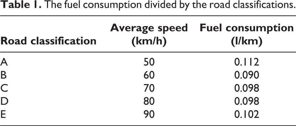
The traditional LRP focuses on transportation cost minimization that depends on distance; however, this study focuses on emission costs that vary by fuel consumption. The fuel consumption rate directly depends on the road classification. For instance, there are two routes traveling from field X to field Y, as shown in Figure 2. The traveling distances of route no. 1 and no. 2 are 24 km and 26 km, respectively. The road classifications of route no. 1 and no. 2 are A and B, respectively. The fuel consumption is calculated by the traveling distance multiplied by the fuel consumption rate, thus the fuel consumption of route no. 1 (2.688 l) is greater than for route no. 2 (2.340 l) even though it is a shorter path, as detailed in Table 2. Therefore, the model will choose route no. 2 for transportation. This illustrates the difference between this study and a traditional LRP. Finally, the emission cost is converted from the fuel used amount (liter), which differs on each route.

Figure 2.

Illustration of traveling from field X to field Y.

Table 2.

The different perspectives between the classical model and proposed model.

Route	Distance (km)	Road classification	Fuel used (l)	Minimized distance LRP	Minimized fuel LRP
1	24	A (0.112)	2.688	✔
2	26	B (0.090)	2.340		✔

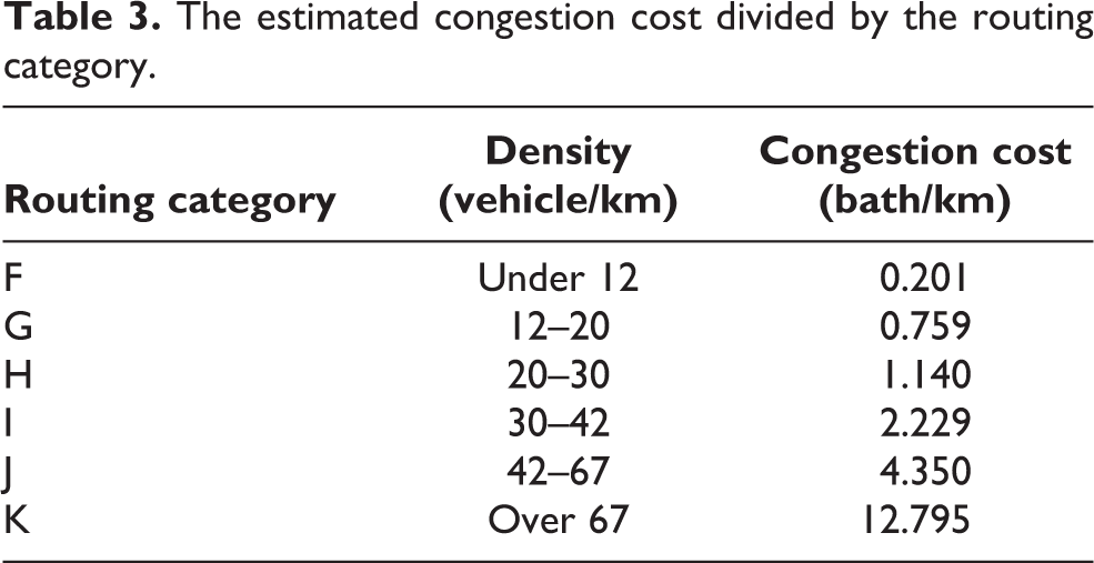
The traffic congestion cost consists of several elements, such as the opportunity cost, delay time, vehicle operating cost, fuel cost, etc. The congestion cost depends on the traffic density of each area as well as the location of the oil palm fields in the study. According to the Victoria Transport Policy Institute,³⁵ the congestion cost can be estimated for different areas and vehicle types. In this report, a quantitative method is approached to estimate congestion cost for various areas using the following elements: (1) a value of travel time of passenger delay, (2) a fuel consumption cost, (3) an accident cost, (4) a reduced business accessibility, and (5) a noise pollution cost. This report also provides a comprehensive overview of external cost estimation and optimal pricing methods, to estimate congestion cost for various vehicle types. Urban areas have high density traffic, and therefore have high congestion costs as well. We adapted the congestion cost from this report, then applied it to our model, as shown in Table 3.

Table 3.

The estimated congestion cost divided by the routing category.

Routing category	Density (vehicle/km)	Congestion cost (bath/km)
F	Under 12	0.201
G	12–20	0.759
H	20–30	1.140
I	30–42	2.229
J	42–67	4.350
K	Over 67	12.795

The mathematical model for MLLRP is declared as follows:

Sets

Vset of nodes, (g, h) $\in$ V and V = I $\cup$ K

Iset of oil palm fields, (i, j) $\in$ I

Kset of extraction plants, k $\in$ K

Parameters

P_i Oil palm quantity of field i

La_j Land price of depot j

Bu_j Construction cost of depot j

Op_j Other operating costs of depot j

d_ij Traveling length in first level from field i to field j, d_ij ⊂ d_gh

d_gh Traveling length in second level from node g to node h

d_jk Traveling length in second level from depotj (located at field j) to plant k d_jk ⊂ d_gh

R_ij Fuel consumption factor in first level from field i to field j, d_ij ⊂ d_gh

R_gh Fuel consumption factor in second level from node g to node h

R_jk Fuel consumption factor in second level from depot j (located at field j) to plant k d_jk ⊂ d_gh

S_ij Congestion cost in first level from field i to field j, d_ij ⊂ d_gh (baht/km)

S_gh Congestion cost in second level from node g to node h (baht/km)

S_jk Congestion cost in second level from depot j (located at field j) to factory k d_jk ⊂ d_gh (baht/km)

q ¹ Vehicle’s loading capacity in first level

q ² Vehicle’s loading capacity in second level

T^D _j Depot’s capacity

T^P _k Extraction plant’s capacity

c ¹Transportation cost in first level (baht/km)

c ²Transportation cost in second level (baht/km)

e ¹Emission cost of fuel used in first level (baht/liter)

e ²Emission cost of fuel used in second level (baht/liter)

Decision variables

n ¹ _i Amount of direct shipments of field i in first level

n ² _j Amount of direct shipments of depot j in second level

z ¹ _ij = 1 if field i is allocated to depot j and direct shipment appears

= 0 otherwise

z ² _jk = 1 if depot j is allocated to plant k and direct shipment appears

= 0 otherwise

x ¹ _ij = 1 if transport from field i to field j and routing for the remaining of direct shipment appears

= 0 otherwise

x ² _gh = 1 if transport from depot j to plant k and routing occurs

= 0 otherwise

z^D _j = 1 if depot j is selected

= 0 otherwise

Support variables

w ¹ _i Remaining quantity after direct shipment at field i in first level

w ² _g Remaining quantity after direct shipment at node g in second level

u ¹ _i Aggregated oil palm quantity in vehicle at field i for sub-tour prevention in first level

u ² _g Aggregated oil palm quantity at node g for sub-tour prevention in second level

m^D _j Amount of round trip of depot j

m^P _k Amount of round trip of plant k

z^P _k = 1 if plant k is selected

= 0 otherwise

Objective function

M i n Z = c^{1} [\sum_{i \in I} \sum_{j \in I} z_{i j}^{1} n_{i}^{1} (d_{i j} + d_{j i}) + \sum_{i \in I} \sum_{j \in I} x_{i j}^{1} d_{i j}] + c^{2} [\sum_{j \in J} \sum_{k \in K} z_{j k}^{2} n_{j}^{2} (d_{j k} + d_{k j}) + \sum_{g \in G} \sum_{h \in G} x_{g h}^{2} d_{g h}] + [\sum_{j \in I} z_{j}^{D} (L a_{j} + B u_{j} + O p_{j})] + e^{1} [\sum_{i \in I} \sum_{j \in I} z_{i j}^{1} n_{i}^{1} (d_{i j} R_{i j} + d_{j i} R_{j i}) + \sum_{i \in I} \sum_{j \in I} x_{i j}^{1} d_{i j} R_{i j}] + e^{2} [\sum_{j \in J} \sum_{k \in K} z_{j k}^{2} n_{j}^{2} (d_{j k} R_{j k} + d_{k j} R_{k j}) + \sum_{g \in G} \sum_{h \in G} x_{g h}^{2} d_{g h} R_{g h}] + [\sum_{i \in I} \sum_{j \in I} z_{i j}^{1} n_{i}^{1} (d_{i j} S_{i j} + d_{j i} S_{j i}) + \sum_{i \in I} \sum_{j \in I} x_{i j}^{1} d_{i j} S_{i j}] + [\sum_{j \in J} \sum_{k \in K} z_{j k}^{2} n_{j}^{2} (d_{j k} S_{j k} + d_{k j} S_{k j}) + \sum_{g \in G} \sum_{h \in G} x_{g h}^{2} d_{g h} S_{g h}]

Constraints

\sum_{j \in I} z_{i j}^{1} = 1 \forall i \in I

P_{i} = n_{i}^{1} q^{1} + w_{i}^{1} \forall i \in I

\sum_{i \in I} z_{i j}^{1} P_{i} = n_{j}^{2} q^{2} + w_{j}^{2} \forall j \in I

\sum_{j \in I, i \neq j} x_{i j}^{1} = \sum_{j \in I, j \neq i} x_{j i}^{1} \forall i \in I

\sum_{g \in G, g \neq h} x_{g h}^{2} = \sum_{g \in G, g \neq h} x_{h g}^{2} \forall h \in V

\sum_{i \in I} z_{i j}^{1} P_{i} \leq z_{j}^{D} T_{j}^{D} \forall j \in I

\sum_{j \in I} z_{j k}^{2} \sum_{i \in I} z_{i j}^{1} P_{i} \leq z_{k}^{P} T_{k}^{P} \forall k \in K

\sum_{k \in K} z_{j k}^{2} = z_{j}^{D} \forall j \in I

\sum_{i \in I, i \neq j} x_{i j}^{1} = (1 - z_{j}^{D}) + z_{j}^{D} m_{j}^{D} \forall j \in I

x_{i j}^{1} \leq \sum_{j \in I} z_{i j}^{1} z_{l j}^{1} \forall i \in I, \forall l \in I

\sum_{g \in G, g \neq k} x_{g k}^{2} = (1 - z_{k}^{P}) + z_{k}^{P} m_{k}^{P} \forall k \in K

x_{g h}^{2} \leq \sum_{k \in K} z_{g k}^{2} z_{h k}^{2} \forall g \in I, \forall h \in I

w_{i}^{1} \leq u_{i}^{1} \leq q^{1} \forall i \in I

u_{i}^{1} + w_{l}^{1} \leq u_{l}^{1} + M (1 - x_{i j}^{1}) \forall i \in I, \forall j \in I i \neq j

w_{g}^{2} \leq u_{g}^{2} \leq q^{2} \forall g \in V

u_{g}^{2} + w_{g}^{2} \leq u_{g}^{2} + M (1 - x_{g h}^{2}) \forall g \in V, \forall h \in V g \neq h

x_{i j}^{1}, x_{g h}^{2}, z_{i j}^{1}, z_{j k}^{2}, z_{j}^{D}, z_{k}^{P} \in \{0, 1\} \forall i, j \in \{1, \dots M\}, \forall k \in \{1, \dots N\}

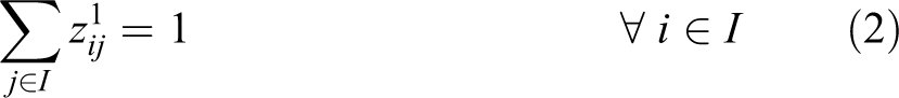
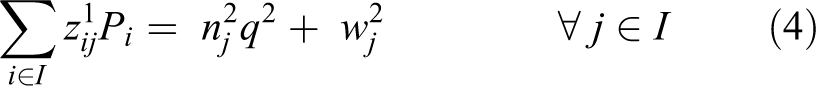
The objective function is defined by equation (1), the goal is to minimize the total cost. The first part and second part are the transportation cost for first level and second level, respectively. The third part is the opening cost of the depot. The fourth part and the fifth part are the emission cost minimization in the first level and second level, respectively. The sixth part and seventh part minimize the congestion cost in the first level and second level, respectively. Constraint (2) states that a field can be assigned to a depot only. If the product quantity is over the capacity of vehicle, Constraints (3) and (4) calculate the number of direct shipments and the remaining oil palm in the first level and second level, respectively. Constraints (5) and (6) guarantee that all routes must start and end at the same node of both field and depot, respectively. Constraints (7) and (8) ensure that the capacity of the depot and extraction plant, respectively, must never be exceeded. Constraint (9) states that a depot can be assigned to one plant only. Constraint (10) routes paths from field to field to collect oil palm. Constraint (11) routes paths to collect oil palm from the assigned field to the depot. Constraint (12) routes paths from depot to depot. Constraint (13) route paths from the assigned depot to the plant. Constraints (14) and (15) specify that the capacity of a vehicle must never be exceeded and the sub-tour prevention constraint in the first level. Constraints (16) and (17) define that the capacity of a vehicle must never be exceeded and the sub-tour prevention constraint in the second level. The binary variables are defined by constraint (18).

For solving the MLLRP problem, Lingo version 11 for Windows was used for finding the optimal solution. Lingo obtains a solution efficiently for small-size problems. As Lingo uses the exact method to find the best solution, it consumes excessive CPU time when the problem size is larger. Therefore, an effective metaheuristic was developed for solving the large-size problem within a reasonable CPU time.

Methodology

The proposed method combines the concept of two well-known metaheuristics, the variable neighborhood search (VNS) and the adaptive large neighborhood search (ALNS). The algorithm operates as follows (see Algorithm 1). It begins from an initial solution, and then a set of neighborhood structures is generated for the shaking phase. The algorithm selects a neighborhood structure randomly at each iteration to expand the searching space. In the local search phase, we applied a destroy and repair operator to improve the solution. The selection of an operator depended on a weight that reflected its performance in the past and this is automatically adjusted periodically. After a local search, if the new solution is worse than the previous one, the acceptance criterion will be applied for whether to continue with the new solution or the previous one.

Algorithm 1

Hybrid algorithm


Input: a set of neighborhood structure N = {N₁, N₂, N₃, N₄, N₅, N₆} Generate initial solution S S_best = S repeat i ← 1 while i $\leq$ i_max do S’← Shaking (S, N₁, N₂, N₃, N₄, N₅, N₆) Setting weight and score of each operator Select d $\in$ D, r $\in$ R S’’ ← r(d(S’)) if C(S’) < C(S’’) then S’ = S’’ end if if accept (S, S’) then S = S’ if C(S) < C(S_best) then S_best = S end if end if adjust weight and score of each operator end while until termination condition is met return S_best

Input: a set of neighborhood structure N = {N₁, N₂, N₃, N₄, N₅, N₆} Generate initial solution S S_best = S repeat i ← 1 while i

\leq

i_max do S’← Shaking (S, N₁, N₂, N₃, N₄, N₅, N₆) Setting weight and score of each operator Select d

\in

D, r

\in

R S’’ ← r(d(S’)) if C(S’) < C(S’’) then S’ = S’’ end if if accept (S, S’) then S = S’ if C(S) < C(S_best) then S_best = S end if end if adjust weight and score of each operator end while until termination condition is met return S_best

Initial solution construction

An initial solution is created by the following constructive heuristic below:

Sum up the product quantity to obtain a number of opened depots and extraction plants. Each depot is set to store a product quantity at least 80% of the maximum capacity. The capacities of the depots and plants are predefined.

Randomly select depots to be opened one by one

Randomly select plants to be opened one by one

Assign each oil palm field to an opened depot using the nearest location, while considering the depot capacity.

Arrange a transportation route in the first level by applying the saving algorithm,³⁶ while considering the vehicle capacity.

Assign each depot to an opened extraction plant using the nearest location, while considering the plant capacity.

Apply step 5 to arrange a transportation route in the second level.

Figure 3 shows an example of an initial solution of the MLLRP.

Figure 3.

Example of an initial solution.

Shaking phase

We designed difference six neighborhood structures to demonstrate the algorithm on the current solution and increase the perturbations. At each iteration, the algorithm randomly selected one of the neighborhood structures for shaking. This phase was intended to diversify into other searching spaces when trapped in a local optima. These neighborhood structures are explained below.

(N₁) Exchange nodes within: Swapping two random nodes (fields or depots) within the same depot or plant. This also includes a field or depot relocation. A depot or plant is chosen with a random probability. If a depot is chosen, two assigned fields at this depot will be swapped. On the other hand, if a plant is chosen, two assigned depots at this plant will be swapped. All related fields will be re-assigned.

(N₂) Exchange nodes between: Swapping two random nodes (fields or depots) between two different depots or plants at the same level. This neighborhood works as with exchange nodes within segments; however, the exchange crosses over different segments. A field or depot is selected with a random probability. If a field is selected, this field will be swapped with another field that is assigned to a different depot. If a depot is selected, this depot will be swapped with another depot that is assigned to a different plant.

(N₃) Change two depots’ status: Randomly select one opened depot and one closed depot (field), then close the current depot and open a new one. As the capacity of a depot is predefined and equivalent at all depots, the number of opened depots stays the same and the solution is always feasible. After opening new depot, the reassignment of nodes and routes are executed in a cost saving manner.

(N₄) Change depot status: Randomly selects a depot at random for changing its status. If its status is open, then close it or vice versa, considering the capacity. As change two depots status tries to maintain the number of opened depot and reassign fields and routes to new depot. This neighborhood allows to change the numbers of opened depots.

(N₅) Change two plants’ status: Similar to changing the two depots status, this structure selects one opened plant and one closed plant then closes the current depot and opens a new one, ensuring that the plant capacity is still not exceeded. After opening a new plant, it aims to minimize the total costs by rearranging the routes to it. After that, the number of opened and closed plants remains the same. If all plants are already opened, the next neighborhood “Change plant status” will be executed instead.

(N₆) Change plant status: This structure is the same concept as the change depot status, but this randomly selects a plant for changing the status. In the case of opening, existing routes in first level are reallocated to the new opened plant in a cost saving manner. Whereas, in the case of closing, the related routes are reallocated to other opened plants. The capacity constraint must also be satisfied.

Local search phase

This phase aims to reach the intensification concept. The idea of ALNS is applied to search for a solution in the different neighborhood structures. The destroy and repair methods are used as local search concepts to improve the solution. In this paper, four destroy and repair operators were developed. We let D = {d_i | i = 1,…, 4} be a set of destroy operators and R = {r_i | i = 1,…, 4} be a set of repair operators. At each iteration, a pair of operators is selected with a probability based on the weight. The initial weight of each operator is set equally but will be adjusted at the end of iteration depending on the quality of the new solution. The highest performance operator will be rewarded with a higher score; thus, it has a high opportunity to be selected repeatedly at the next iteration. These destroy and repair operators are described below.

Destroy operator.

The destroy operator is used to ruin the solution and then turns incomplete. This method perturbed the current solution to search at a variety of areas. The destructive degree is denoted by d_d = {10%, 15%, 20%, 25%, 30%}, which defines the size of destruction. For instance, if the solution contains 20 fields and d_d = 20% is selected randomly, then four fields (20 × 20%) will be removed from current solution. After destruction, a repair operator will be executed to re-construct a new solution of the problem, which will be described in the next section.

1) Random removal

This operator works by randomly selecting q fields and putting them into the field pool as shown in Figure 4.

Figure 4.

Example of random removal.

2) Connected removal

The connected removal randomly selects a field, called a seed field, and the q-1 fields that are closest to the seed field are marked. Then, all these fields are removed from the current solution and put into the field pool as shown in Figure 5.

Figure 5.

Example of connected removal.

3) Worst removal

This operator finds the worst fields to be removed by calculating the total cost without a field in the current solution one by one. Then, this calculates the difference cost between when a field is in the solution and when it is taken off. The q fields that own the highest different cost will be removed from the current solution.

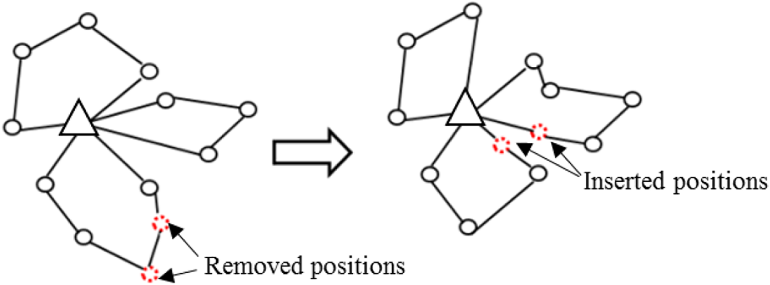
4) Fixed zone removal

Fixed zone removal was developed to destroy the solution in a specified area, called the fixed zone. The main idea is to let the solution move to a proper direction until it finds the best solution. In other words, this operator avoids the random walk search in the solution. The fixed zone removal works with the following steps:

Separate the fields by four zones based on its actual location, the latitude and longitude, as shown in Figure 6.

Randomly choose the fixed zone area (f_a), f_a = {1,2,3,4). This is the zone that will be destroyed.

Randomly select a destroyed operator (random removal, worst removal, or connected removal).

Execute the selected destroy operator to remove the fields within the fixed zone in step 2.

Figure 6.

Fixed zone area.

Repair operator.

The repair operator is used to re-insert the part of the solution that is removed by the destroy operator. Each operator owns different insertion methods for improving the new solution.

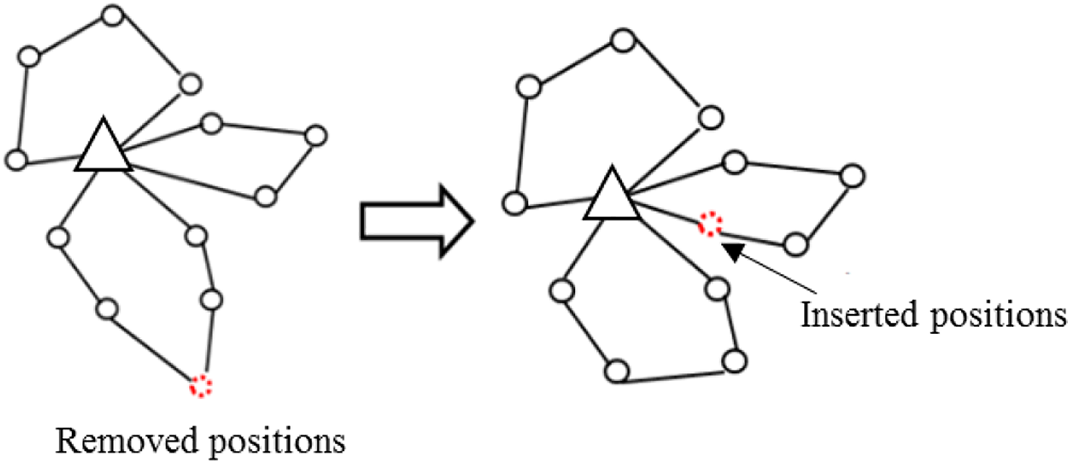
1) Random insertion

Random insertion is a simple and uncomplicated method. The operator brings the removed fields back to the solution at any position, regardless of the objective value. Figure 7 shows the characteristics of the random insertion operator.

Figure 7.

Characteristics of random insertion operator.

2) Forbidden insertion

This operator performs same concept as the random insertion, but it is not allowed to re-insert into the same depot that it was in before the destroy operation. This forces the searching area of the new solution to be changed. This operator was developed primarily for diversification purposes.

3) Best insertion

For the best insertion, the operator determines the best position that obtains the lowest cost. This inserts the fields in a random order one by one until there are no fields left in the pool. Figure 8 shows an example of best insertion operator.

Figure 8.

Characteristics of the best insertion operator.

4) Swap

Swap is a simple and well-known local search method. This operator is used for exchanging the selected fields, which are then turned into the new solution, as shown in Figure 9. The steps of the swap method are as follows:

Select 2–3 fields randomly.

Mark the position of those fields to identify the position of the fields.

Exchange the field position as the identified point.

Figure 9.

Characteristics of the swap operation.

Solution acceptance

Generally, the ALNS procedure contains the acceptance criterion to perform a determination for every new solution at each iteration. After the repair operation, a new solution will be obtained, if it is better than the original one, it will proceed to the next iteration. In the case of the worse solution, the solution acceptance will be conducted to provide a chance for acceptance with a small probability. In this paper, we adopted a popular criterion for ALNS, simulated annealing (SA), as the solution acceptance method. The non-improving solution was tested with probability $p = e x p (z (s) - z (s^{'})) / k T$ , where T is the temperature at each iteration. This was maximally set at the first iteration, then, decreased constantly at every next iteration and k was the constant value used to control the reduction of temperature. With regard to acceptance method at the beginning, the probability p to accept non-improving solution is high and decrease slowly, the probability of acceptance decreases dramatically. The purpose is to allow the algorithm accepts a marginally worse solution than the current one and to let it focus on more improving solutions later on.

Experimental results

In this paper, the efficiency of the hybrid algorithm (HA) was presented for solving a multi-level location routing problem by comparing with the solution from Lingo for Windows, which is an exact methodology. The mathematical model and proposed algorithm were coded on Windows operation using a personal computer with Intel Core i5 CPU 2.7 GHz Ram DDR4 16 GB. The three groups of testing instances were randomly generated, and the details of the testing instances are shown in Table 4. The sizes of the instances were divided into small, medium, and large according to the number of fields and the number of plants. The stopping criteria of Lingo was the computational time, which was set differently depending on the instance size.

Table 4.

Testing instance data.

Instance	Number of fields	Number of plants	Instance	Number of fields	Number of plants	Instance	Number of fields	Number of plants
SM1	4	2	ME1	10	4	LA1	20	7
SM2	4	2	ME2	12	4	LA2	20	7
SM3	5	3	ME3	13	3	LA3	25	8
SM4	5	3	ME4	14	5	LA4	25	8
SM5	6	2	ME5	15	4	LA5	30	8
SM6	6	3	ME6	16	4	LA6	30	7
SM7	7	4	ME7	16	5	LA7	35	8
SM8	8	2	ME8	17	4	LA8	35	7
SM9	8	3	ME9	18	6	LA9	40	8
SM10	9	4	ME10	19	6	Case study	120	8

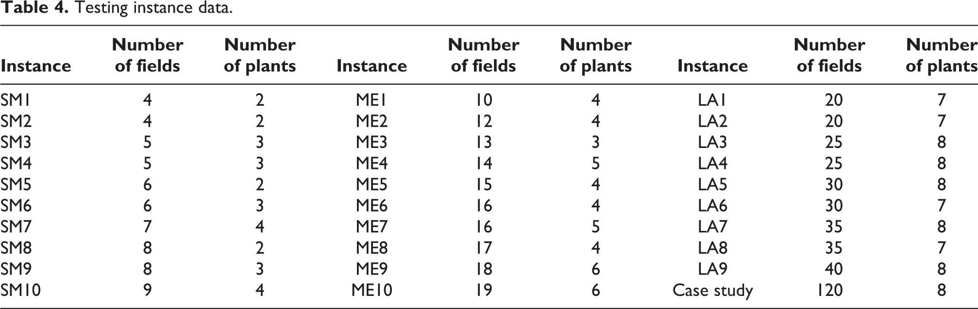
For a small-size instance, the computational time was recorded when finding an optimal solution. For medium and large-size instances, the computational time was limited to 48 h and 96 h, respectively. However, the stopping criteria of HA was the number of iterations or computational limited time, which depended on the purpose of each experiment. This will be explained next. The proposed HA was coded by Visual studio 2019 and was tested for three runs per experiment; then, the average result was reported. The statistical test was conducted via MINITAB® (Minitab Inc.) at the 95% confidence interval.

The first experimental result was a comparison of the solutions obtained by Lingo and the proposed algorithm as shown in Table 5. The stopping criteria of the proposed algorithm was set at 5000 iterations. For small-sized instances, Lingo was able to obtain the optimal solution; thus, the results of HA could be compared with the optimal solution. Both methods could find the same results within a short computational time.

Table 5.

The computational results of the testing instance and case study.

	Lingo			Hybrid Algorithm (HA)		% gap^(d)
Instance	Total cost (baht)	Computational time (min)	Status	Total cost (baht)	Computational time (min)	Total cost
SM1	80884.03	0.37	Opt^(a)	80884.03	1.04	0.00
SM2	80805.72	0.67	Opt	80805.72	1.04	0.00
SM3	161255.68	0.22	Opt	161255.68	1.04	0.00
SM4	163426.08	0.30	Opt	163426.08	1.04	0.00
SM5	162422.71	0.30	Opt	162422.71	1.04	0.00
SM6	161590.62	2.44	Opt	161590.62	1.04	0.00
SM7	161536.90	2.44	Opt	161536.90	1.63	0.00
SM8	241864.51	1.48	Opt	241864.51	1.48	0.00
SM9	241755.49	2.66	Opt	241755.49	1.63	0.00
SM10	161755.49	3.03	Opt	161755.49	1.11	0.00
Average	161729.72	1.39		161729.72	1.21	0.00
ME1	241869.94	2880	BSF^(b)	232113.49	1.78	−4.20
ME2	241758.10	2880	BSF	233591.32	1.78	−3.50
ME3	163819.08	2880	BSF	155722.28	3.61	−5.20
ME4	243491.88	2880	BSF	241229.86	3.42	−0.94
ME5	163589.93	2880	BSF	155089.93	3.76	−5.48
ME6	243806.05	2880	BSF	239412.16	3.58	−1.84
ME7	243741.31	2880	BSF	234763.76	3.19	−3.82
ME8	164028.43	2880	BSF	155076.20	3.49	−5.77
ME9	244044.69	2880	BSF	234924.45	3.51	−3.88
ME10	164259.97	2880	BSF	160181.85	3.48	−2.55
Average	211440.94	2880		204210.53	3.16	−3.72
LA1	243218.70	5760	LB^(c)	257329.78	9.75	5.48
LA2	324096.68	5760	LB	340467.17	9.78	4.81
LA3	322942.60	5760	LB	350868.80	8.06	7.96
LA4	242622.72	5760	LB	268610.28	9.32	9.67
LA5	245289.72	5760	LB	259658.91	9.41	5.53
LA6	322726.31	5760	LB	333918.35	8.76	3.35
LA7	322565.82	5760	LB	334732.88	9.63	3.63
LA8	332388.94	5760	LB	346995.87	9.75	4.21
LA9	414207.23	5760	LB	439000.49	10.48	5.65
Case study	819183.08	5760	LB	877260.23	15.84	6.62
Average	358924.18	5760		378556.48	10.08	5.69

(a) = Optimal solution, (b) = Best solution found during limited time, (c) = Lower bound of solution, (d) = Percentage difference between result from proposed algorithm and Lingo, whereas $% g a p = (\frac{S_{H A} - S_{L i n g o}}{S_{H A}}) \times 100$ .

For medium and large-size instances, Lingo was not able to obtain the optimal solution within a reasonable time; therefore, the results of HA were compared with the BSF (best solution found during a limited time) and LB (lower bound of solution), which were obtained in 48 h and 96 h of running time, respectively. The positive sign (+) of %gap indicated that the HA result was better than the Lingo result because the BSF was not the optimal solution. On the other hand, the negative sign (−) of %gap indicated that the HA result was worse than the Lingo result because the LB was the lowest boundary of solution. From these results, the Wilcoxon’s signed rank test was conducted to verify the significant difference between the Lingo and HA result, the p-value is shown in Table 6.

Table 6.

Wilcoxon’s signed rank test for the results given by Table 5.

	Total cost	Computational time
Small	N/A	0.441
Medium	0.006	0.006
Large	0.006	0.006

In terms of the objective value, the HA significantly improved the solution quality from the BSF obtained by Lingo in a medium-sized instance, with the average percentage differences (%gap) at −3.72%. For a large-sized instance, Lingo’s outcome was significantly better than HA but the solution’s status was only lower bound. The average %gap was not far; it was only 5.69%.

In terms of the computational time, this was not significantly different for both methods in small-sized instances. However, for medium and large-sized instances, HA used less processing time than Lingo, at 99.89% ((2880 – 3.16)/2880) and 99.83% ((5760 – 10.08)/5760), respectively.

From the %gap results, we performed ANOVA (analysis of variance) to check if the %gap was significantly different when the instance size was changed. The hypothesis test was declared as follows:

H_{0} : μ_{S M} = μ_{M E} = μ_{L A}

H_{a} : μ_{S M} \neq μ_{M E} \neq μ_{L A or the means are not all equal}

The p-value of the ANOVA test was 0.000, which indicates that the HA performed significantly differently compared to the results from Lingo when the instance size was changed. Figure 10 shows the Tukey comparison result. The interval did not contain zero; thus, the corresponding means were significantly different for all pairs.

Figure 10.

The Tukey results from the ANOVA test.

The experimental results shown in Table 7 reveal the duration for the methods that found the best solution in small-sized instances. This experiment aimed to assess which method consumed the shortest duration to find the optimal solution. The stopping criteria of HA were the same as for the previous results; however, the time when to find the best solution was reported. The statistical test was Wilcoxon’s signed rank test method to compare the different durations. The p-value was equivalent to 0.032, which was less than the significance level. Therefore, the HA method was significantly faster than Lingo when searching the same solution quality.

Table 7.

The processing time when finding the best solution.

Instance	Total cost (baht)	Lingo Time (min)	Hybrid algorithm (HA) Time (min)
SM1	80884.03	0.37	0.25
SM2	80805.72	0.67	0.48
SM3	161255.68	0.22	0.33
SM4	163426.08	0.30	0.26
SM5	162422.71	0.30	0.47
SM6	161590.62	2.44	0.53
SM7	161536.90	2.44	0.65
SM8	241864.51	1.48	0.75
SM9	241755.49	2.66	0.87
SM10	161755.49	3.03	0.63
Average		1.39	0.52
P-value of wilcoxon’s signed rank test = 0.032

The last experiment was conducted on medium and large-sized instances to verify the solution quality when extending the duration. The computational time was set to 20 and 30 min for medium and large-sized instances as the stopping criteria. The results are shown in Table 8.

Table 8.

Experimental results while testing the fixed computational time.

	Lingo			Hybrid algorithm
Instance	Total cost (baht)	Computational time (min)	Status	Total cost (baht)	Computational Time (min)
ME1	241869.94	2880	BOF	232113.49	20
ME2	241758.10	2880	BOF	233591.32	20
ME3	163819.08	2880	BOF	155722.28	20
ME4	243491.88	2880	BOF	241229.86	20
ME5	163589.93	2880	BOF	155089.93	20
ME6	243806.05	2880	BOF	239412.16	20
ME7	243741.31	2880	BOF	234763.76	20
ME8	164028.43	2880	BOF	155076.20	20
ME9	244044.69	2880	BOF	234924.45	20
ME10	164259.97	2880	BOF	159893.28*	20
LA1	243218.70	5760	LB	257329.78	30
LA2	324096.68	5760	LB	340467.17	30
LA3	322942.60	5760	LB	332678.62	30
LA4	242622.72	5760	LB	259960.01	30
LA5	245289.72	5760	LB	259658.91	30
LA6	322726.31	5760	LB	331762.38	30
LA7	322565.82	5760	LB	334732.88	30
LA8	332388.94	5760	LB	346995.87	30
LA9	414207.23	5760	LB	439000.49	30
Case study	819183.08	5760	LB	865822.52	30

* Bold numbers indicate that it is improved solution comparing to the results from fixed iteration experiment.

Wilcoxon’s signed rank test was conducted to check whether the proposed HA was dissimilar in performance for both sizes. The p-values are shown in Table 9.

Table 9.

Statistical test while using a fixed computational time.

Instance size	p-value
Medium	0.006
Large	0.006

The results demonstrated that the proposed HA generated a solution that was significantly different to the solution obtained by Lingo. However, HA gave a better solution than Lingo, which obtained only BSF. In this experiment, HA improved five solutions from 20 instances comparing to the results from the fixed iteration experiment in Table 5, with 25% improvement.

The proposed HA was deployed for solving the case study problem to decide the depot location and manage the transportation routes. For the first level, the algorithm decided to open 10 depots as the collecting points for oil palm and provided 24 different routes to transport the oil palm from field to depot, as shown in Table 10. For second level, the algorithm decided to open five extraction plants and provided 10 different routes to transport the oil palm from depot to extraction plant, as shown in Table 11. The total cost in the objective function was minimized at each route for both levels. The total cost of the case study was 865,822.52 baht, which was acquired from the summation of both levels (848,953.55 + 16,868.97).

Table 10.

The results of the case study at the first level.

Routing no.	Opened depot	Routing	Total cost (baht)
1	7	7—4—7	81,856.32
2		7—4—1—7	1,712.38
3		7—99—93—102—105—103—115—109—98—106—113—116—110—39—97—96—100—101—7	2,609.43
4	10	10—20—22—21—10	81,982.45
5		10—20—18—14—12—2—10	1,690.43
6	15	15—16—15	81,892.04
7		15—13—44—15	2,098.34
8		15—112—111—15	1,938.92
9	17	17—41—40—90—17	82,193.76
10		17—23—27—30—28—31—29—17	2,056.91
11		17—19—3—8—9—17	2,135.61
12	36	36—84—81—83—82—85—55—36	82,056.22
13	45	45—87—86—88—32—35—34—33—24—25—38—91—92—89—45	82,591.72
14		45—42—43—37—26—45	1,822.54
15	49	49—47—49	81,808.83
16		49—46—50—48—47—49	1,921.81
17		49—108—107—114—104—56—57—58—95—49	2,276.31
18	74	74—76—53—6—5—74	82,031.92
19		74—69—72—71—68—74—59—60—61—62—63—74	2,281.16
20	80	80—75—52—11—94—73—80	82,031.88
21		80—54—51—70—79—77—80	2,241.80
22		80—64—65—66—67—80	1,943.86
23		80—78—80	1,672.63
24	119	119—120—117—118—119	82,106.28
		Total	848,953.55

Table 11.

The results of the case study at the second level.

Routing no.	Opened plant	Routing	Total Cost (baht)
1	1	1—7—1	1,602.77
2		1—7—10—1	1,766.25
3	2	2—15—2	1,642.34
4	4	4—17—4	1,798.31
5		4—36—4	1,593.48
6		4—45—4	1,621.56
7		4—49—4	1,732.71
8	6	6—74—6	1,709.26
9		6—80—6	1,692.96
10	7	7—119—7	1,709.33
		Total	16,868.97

The overall results indicate the proposed HA is efficient and suitable for solving complex problem especially the multi-level LRP, comparing to Lingo software. The HA performance is justified by small differences from Lingo’s results, but it can save huge gap of time consumption when the problem size is larger. The HA combines strength point of two well-known metaheuristics. The core concept of VNS is to randomly move the algorithm in various neighborhoods of expanding size as diversification mechanism, whereas the ALNS is aimed to find the optimal solution intently by various strategies, the most powerful strategy has a great opportunity to apply frequently. The key successes of HA are its ability to move to divers searching areas by applying different six neighborhood structures and its ability to intend to find the best solution in specified area by applying four destroy and repair methods.

Recently, Pitakaso et al.³⁷ introduced a new type of metaheuristic called the variable neighborhood strategy adaptive search (VaNSAS) as a solution approach for solving the green two-echelon location routing problem (G2ELRP). Table 12 shows the performance comparison between the proposed HA and VaNSAS in terms of percent difference (% gap) from Lingo’s solution. The statistical test of mean difference revealed the p-value was equal 0.166. Hence, we concluded that both methods were not significantly different regarding the percentage difference from Lingo. However, both studies contained different sizes of instances, including the product quantity, number of fields, and number of plants, as well as the limited time in the experiment. These may have impacted the comparison results.

Table 12.

Comparison of the results with recent research.

VaNSAS		HA
Instance	%gap	Instance	%gap
L1	3.34	LA1	5.48
L2	8.29	LA2	4.81
L3	9.21	LA3	7.96
L4	11.39	LA4	9.67
L5	6.52	LA5	5.53
L6	6.58	LA6	3.35
L7	9.43	LA7	3.63
L8	4.67	LA8	4.21
L9	5.29	LA9	5.65
L10	3.26	—	—
case study	17.53	case study	5.69
Average	7.77	Average	5.60
p-value of two sample t-test = 0.166

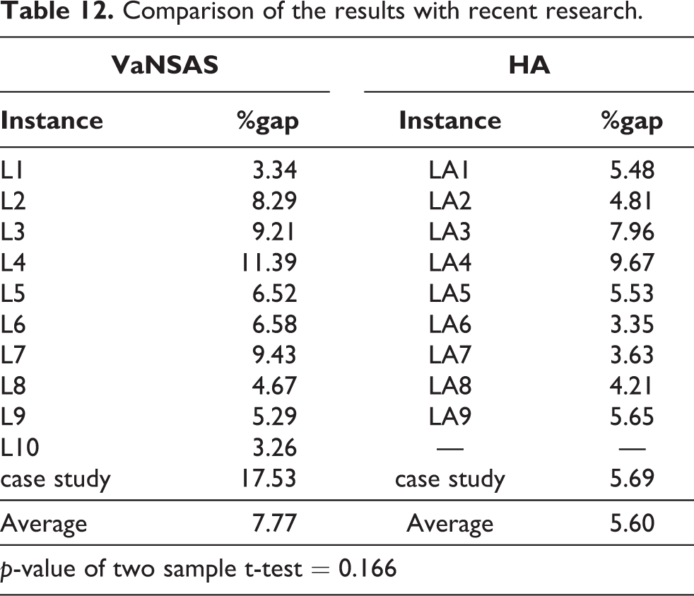
Table 13 showed the comparison results of HA and various methods in the literature that proposed for solving environmental impact characteristics. We compare HA method with VaNSAS (Pitakaso et al.) and ALNS (Demir et al.),³⁸ % gap is the percentage difference between results obtained by proposed methods and exact method (Lingo/CPLEX). The HA obtained the best solution’s quality comparing to the other methods because %gap is only 5.69%. However, all studies contained different sizes of instances, including the product quantity, number of fields, and number of plants, as well as the limited time in the experiment. These may have impacted on the comparison results.

Table 13.

Comparison of the results with other methods for solving environmental impact.

			Minimization of
Author	Proposed method	Single-level/multi-level	Fuel	Emission	Congestion	Operational Cost	Number of nodes	CPU time (s)	Number of iterations	% gap
Pitakaso et al. (2020)	VaNSAS	Multi	✔				116	1,099.2	10,000	17.53
Demir et al. (2012)	ALNS	Single	✔	✔			100	145.3	N/A	9.35
Our study	HA (VNS+ALNS)	Multi	✔	✔	✔	✔	120	950.4	5,000	5.69

Finally, in order to test the performance of the proposed algorithm, we performed the test on the standard instances for two-echelon LRP that was derived from Phodhon’s benchmarks.¹¹ We tested five runs for each instance and recorded the best total cost and CPU time. The results are presented in Table 14. The HA was compared with GRASPxLP (Nguyen et al.),¹⁷ MS-ILS (Nguyen et al.),¹⁸ Hybrid SA (Pichka et al.)¹³ and two-phase method (TPM) (Dai et al.).³⁹ Column 1 and 2 define instance name and best-known solution (BKS) obtained by previous literature. In term of CPU time, TPM is the fastest in all methods as the average time of GRASPxLP, MS-ILS, Hybrid SA, TPM and HA is 22.62 s, 423.50 s, 31,260 s, 7.54 s and 8.73 s, respectively. The HA is the second best with the average difference is only 1.09 s (8.73–7.54). In term of solution’s quality, MS-ILS is the best performance in all methods since the average %gap of GRASPxLP, MS-ILS, Hybrid SA, TPM and HA is 1.16%, 0.12%, 1.04%, 2.63%, and 2.72%, respectively. HA is competitive to TPM as the average difference is only 0.09 s (2.72–2.63). Although GRASPxLP and MS-ILS and Hybrid SA are better than TPM and HA, but they consume high processing time. Thus, if the requirement of solution’s quality is not very high, HA can be acceptable. Besides fast speed of operation, HA is easy to use as it does not require tuning or setting the parameters of algorithm.

Table 14.

Results for two-echelon LRP testing on Prodhon’s benchmarks.

		GRASPxLP			MS-ILS			Hybrid SA			TPM			HA
Instances	BKS	Total cost	CPU time (s)	% gap	Total cost	CPU time (s)	% gap	Total cost	CPU time (s)	% gap	Total cost	CPU time (s)	% gap	Total cost	CPU time (s)	% gap
200-10-1a	557,099	570,210	26.50	2.35	559,428	553	0.42	561,835	36780	0.84	561,840	8.15	0.85	563,803	9.52	1.55
200-10-1b	452,286	454,181	20.60	0.42	452,731	673	0.10	460,476	26880	1.78	466,288	7.51	4.34	465,786	8.64	2.89
200-10-2a	502,333	508,450	22.40	1.22	502,400	211.1	0.01	506,124	37380	0.75	505,700	7.52	0.67	507,845	7.16	1.06
200-10-2b	425,311	429,075	21.90	0.88	425,311	248.1	0.00	429,033	25440	0.87	428,749	7.67	0.80	431,247	8.62	1.38
200-10-3a	533,732	541,754	26.00	1.50	533,732	632.9	0.00	543,312	36300	1.76	546,708	7.31	2.38	545,821	9.51	2.23
200-10-3b	419,047	421,585	18.30	0.61	419,790	222.9	0.18	419,961	24780	0.22	451,278	7.07	6.74	451,884	8.93	7.25
Average			22.62	1.16		423.50	0.12		31,260	1.04		7.54	2.63		8.73	2.72

Conclusion and suggestion

This research studied a multi-level location routing problem (MLLRP) considering the environmental impact by including the emission cost and congestion cost in the objective function. The problem is considered complicated as it concerns the decision of location and routing in both levels. The depot locations must be determined from the potential fields established, and then the vehicle routes are provided for collecting the oil palm from farmers to the opened depots. After that, the extraction plants must be selected along with the vehicle routes to transport the oil palm from the opened depot to the selected plants.

The mathematical model was formulated with the purpose of total cost minimization. The model was tested using the Lingo program with three groups of testing instances, which contained different problem sizes. Although Lingo was recognized as able to find an exact solution, it was not suitable for large problems due to the unreasonable processing time. Therefore, we developed a hybrid metaheuristic for solving the MLLRP.

The proposed algorithm can solve the problem efficiently compared to Lingo’s solution. There was no gap in small-sized instances, and it outperformed Lingo’s solution in medium-sized instances. For large-sized instances, although Lingo’s solution was better than the proposed algorithm, it was lower bound in the solution. The proposed algorithm consumed approximately 99% less processing time than Lingo.

For benchmarking purposes, we compared the performance of the proposed method with another method in the related literature. The result revealed that our method was not significantly different from the method in the recent literature in terms of the solution quality. Finally, the proposed algorithm was applied to the case study problem for managing the locations of the depots, extraction plants, and transportation routes for both levels. This study will aid sustainable development in the agriculture industry by reducing the transportation costs for farmers and related collaborators and by decreasing the environmental harmfulness as well. This study can be adapted not only to the agricultural industry but also to other industries in Thailand or around the world.

For future research, the consideration of additional factors that affect the emission cost and congestion cost would be valuable. These factors will allow the model to further approach the realistic problem. Other real-world constraints, such as time windows, stochastics demands, and heterogeneous fleets of vehicles should be included into the model. Another beneficial avenue for future study is to develop other new hybrid algorithms to accelerate the computational time.

Footnotes

Declaration of conflicting interests

The author(s) declared no potential conflicts of interest with respect to the research, authorship, and/or publication of this article.

Funding

The author(s) received no financial support for the research, authorship, and/or publication of this article.

ORCID iD

Chalermchat Theeraviriya

References

Krungsri Research. Oil palm industry. Thailand industry outlook 2016–2018. https://www.krungsri.com/bank/getmedia/47653083-c572-410f-944c-5da99c47aed8/IO_Oil_Palm_200124_TH_EX.aspx (2018, accessed on 9 July 2020).

FAOSTAT. Food and Agriculture Organization of the United Nations: Rome. Electronic crop data. http://www.fao.org/faostat/en/#data/QC (2020, accessed on 9 July 2020).

Jensen

Keogh-Brown

Shankar

, et al. Palm oil and dietary change: application of an integrated macroeconomic, environmental, demographic, and health modelling framework for Thailand. Food Policy 2019; 83: 92–103.

Nootim

Kongkaew

Sirivongpaisal

, et al. An application of zoning designated policy to locate the fresh fruit bunch collectors in the oil palm supply chain: Southern Thailand case study. In: IOP Conference Series: Materials Science and Engineering, Medan City North Sumatera, Indonesia, 16 October 2018, DOI: 10.1088/1757-899x/505/1/012121.

Nootim

Kongkaew

Sirivongpaisal

, et al. A Location analysis of the fresh fruit bunch collectors in oil palm supply chain under zoning designated policy: a case study of Krabi Province. Thai J Oper Res 2018; 6: 32–45.

Demir

Bektaş

Laporte

. The bi-objective pollution-routing problem. Eur J Oper Res 2014; 232: 464–478.

Demir

Bektaş

Laporte

. A comparative analysis of several vehicle emission models for road freight transportation. Transp Res D Transp Environ 2011; 16: 347–357.

Jayasooriya

SACS

Bandara

. Measuring the economic costs of traffic congestion. In: 2017 Moratuwa Engineering Research Conference (MERCon), Moratuwa, Sri Lanka, 29–31 May 2017, pp. 141–146. US: IEEE.

Transport Statistics Sub-Division, Planning Division, Department of Land Transport. Number of registered vehicles. Transport Statistics Sub-Division, Planning Division, Department of Land Transport. https://web.dlt.go.th/statistics/ (2020, accessed on 9 July 2020).

10.

Chen

Cheung

Chu

S-C

, et al. Transshipment hub selection from a shipper’s and freight forwarder’s perspective. Exp Syst Appl 2017; 83: 396–404.

11.

Prodhon

Prins

. A survey of recent research on location-routing problems. Eur J Oper Res 2014; 238: 1–17.

12.

Vidović

Ratković

Bjelić

, et al. A two-echelon location-routing model for designing recycling logistics networks with profit: MILP and heuristic approach. Exp Syst Appl 2016; 51: 34–48.

13.

Pichka

Bajgiran

Petering

MEH

, et al. The two echelon open location routing problem: Mathematical model and hybrid heuristic. Comput Ind Eng 2018; 121: 97–112.

14.

Cuda

Guastaroba

Speranza

. A survey on two-echelon routing problems. Comput Oper Res 2015; 55: 185–199.

15.

Jacobsen

Madsen

OBG

. A comparative study of heuristics for a two-level routing-location problem. Eur J Oper Res 1980; 5: 378–387.

16.

Lin

J-R

Lei

H-C

. Distribution systems design with two-level routing considerations. Ann Oper Res 2009; 172: 329–347.

17.

Nguyen

V-P

Prins

Prodhon

. Solving the two-echelon location routing problem by a GRASP reinforced by a learning process and path relinking. Eur J Oper Res 2012; 216: 113–126.

18.

Nguyen

V-P

Prins

Prodhon

. A multi-start iterated local search with tabu list and path relinking for the two-echelon location-routing problem. Eng Appl Artif Intell 2012; 25: 56–71.

19.

Drexl

Schneider

. A survey of variants and extensions of the location-routing problem. Eur J Oper Res 2015; 241: 283–308.

20.

Yang

Zeng

. Models and methods for two-echelon location routing problem with time constraints in City Logistics. Math Probl Eng 2018; 2018: 2549713–2549713.

21.

Schwengerer

Pirkwieser

Raidl

. A variable neighborhood search approach for the two-echelon location-routing problem. In: Hao

J–k

Middendorf

(eds) European conference on evolutionary computation in combinatorial optimization. Berlin, Heidelberg: Springer Berlin Heidelberg, 2012, pp. 13–24.

22.

Contardo

Hemmelmayr

Crainic

. Lower and upper bounds for the two-echelon capacitated location-routing problem. Comput Oper Res 2012; 39: 185–3199.

23.

Jarboui

Derbel

Hanafi

, et al. Variable neighborhood search for location routing. Comput Oper Res 2013; 40: 47–57.

24.

Macedo

Hanafi

Jarboui

, et al. Variable neighborhood search for the location routing problem with multiple routes. In: Proceedings of 2013 International Conference on Industrial Engineering and Systems Management (IESM), Agdal, Morocco, 28–30 October, 2013, pp. 19–24. US: IEEE.

25.

Hemmelmayr

Cordeau

J-F

Crainic

. An adaptive large neighborhood search heuristic for two-echelon vehicle routing problems arising in city logistics. Comput Oper Res 2012; 39: 3215–3228.

26.

Schiffer

Walther

. An Adaptive large neighborhood search for the location-routing problem with intra-route facilities. Transp Sci 2017; 52: 331–352.

27.

Toro

Franco

Echeverri

, et al. A multi-objective model for the green capacitated location-routing problem considering environmental impact. Comput Ind Eng 2017; 110: 114–125.

28.

Toro

Franco

Granada-Echeverri

, et al. Green open location-routing problem considering economic and environmental costs. Int J Ind Eng Comput 2016; 8: 203–216.

29.

Wang

. Carbon reduction in the location routing problem with heterogeneous fleet, simultaneous pickup-delivery and time windows. Proc Comput Sci 2017; 112: 1131–1140.

30.

Wang

Tao

Shi

. Optimization of location-routing problem for cold chain logistics considering carbon footprint. Int J Environ Res Public Health 2018; 15: 86–86.

31.

Dukkanci

Peker

Kara

. Green hub location problem. Transp Res E Logist Transp Rev 2019; 125: 116–139.

32.

Dukkanci

Kara

Bektaş

. The green location-routing problem. Comput Oper Res 2019; 105: 187–202.

33.

Govindan

Jafarian

Khodaverdi

, et al. Two-echelon multiple-vehicle location-routing problem with time windows for optimization of sustainable supply chain network of perishable food. Int J Prod Econ 2014; 152: 9–28.

34.

Akararungruangkul

Kaewman

. Modified differential evolution algorithm solving the special case of location routing problem. Math Comput Appl 2018; 23: 34–34.

35.

Victoria Transport Policy Institute. Transportation cost and benefit analysis techniques, estimates and implications. https://www.vtpi.org/tca/ (2020, accessed on 9 July 2020).

36.

Clarke

Wright

. Scheduling of vehicles from a central depot to a number of delivery points. Oper Res 1964; 12: 568–581.

37.

Pitakaso

Sethanan

Theeraviriya

. Variable neighborhood strategy adaptive search for solving green 2-echelon location routing problem. Comput Electron Agric 2020; 173: 105406–105406.

38.

Demir

Bektaş

Laporte

. An adaptive large neighborhood search heuristic for the Pollution-Routing Problem. Eur J Oper Res 2012; 223: 346–359.

39.

Dai

Aqlan

Gao

, et al. A two-phase method for multi-echelon location-routing problems in supply chains. Exp Syst Appl 2019; 115: 618–634.

Solving the multi-level location routing problem considering the environmental impact using a hybrid metaheuristic

Abstract

Keywords

Introduction

Literature review

Problem description and model formulation

Methodology

Initial solution construction

Shaking phase

Local search phase

Destroy operator.

Repair operator.

Solution acceptance

Experimental results

Conclusion and suggestion

Footnotes

Declaration of conflicting interests

Funding

ORCID iD

References