
Abstract
The purpose of this study is to explain the following proposition: Profit maximization objective is only an assumption, which is valid only when marginal cost is zero; a firm should maximize its total sales rather than its profit when marginal cost is not equal to zero. Using simple logical consequences, the study shows the following: (i) Cournot equilibrium occurs at total revenue maximization conditions rather than profit maximization conditions, even if costs are not neglected; (ii) if average costs of plants are not equal to each other, a multiple-plant monopoly cannot maximize its profit; it should maximize its total revenue, even if costs are not zero; (iii) a firm’s goal should be total revenue maximization rather than profit maximization, when marginal cost is not equal to zero; (iv) profit maximization behaviour does not have to explain economic growth; however, total sales maximization behaviour clearly explains economic growth and (v) total sales maximization objective, at the producer’s equilibrium conditions, guarantees stability under diminishing returns. The study concludes with nine simple results in order to support its claim. The results of the study emphasize that (i) an empirical analysis based on a strict theory should start to the analysis depending on a goal function which maximizes total sales rather than profit and (ii) a representative social planner who designs a growing economy, which grows thanks to total sales maximization behaviour of firms, should design the economy where price changes do not give advantage to the firms.
Keywords
Introduction
What does a firm maximize? It is frequently assumed that a firm maximizes its own profit. Thus, it is frequently admitted that the aim of a firm is profit maximization. The present study claims that an analysis depending on a goal function which maximizes profit includes fallacy; profit maximization objective is only an assumption which is valid only under certain conditions. Indeed, a firm maximizes its own total revenue or sales. The method of the study does not include topology. Rather than topological explanations, the present article uses simple logical consequences under certain conditions in order to explain its claim, and it briefly attempts to explain the link between total sales maximization behaviour and economic growth.
Based on those logical consequences, the contributions of the study are as follows: (i) Cournot equilibrium occurs at total revenue maximization conditions rather than profit maximization conditions, even if costs are not neglected (note that if costs are zero, then profit has already been equal to total revenue); (ii) if average costs of plants are not equal to each other, a multiple-plant monopoly cannot maximize its profit; it should maximize its total revenue, even if costs are not zero (note that if costs are zero, then profit has already been equal to total revenue); (iii) a firm’s goal should be total revenue maximization rather than profit maximization, when marginal cost is not equal to zero; (iv) profit maximization behaviour does not have to explain economic growth; however, total sales maximization behaviour clearly explains economic growth and (v) total sales maximization objective, at the producer’s equilibrium conditions, guarantees stability under diminishing returns.
Let us give a short explanation and related literature about these five contributions.
The present study emphasizes that each of profit maximization and total sales maximization objectives cannot be an objective by itself, necessarily; the objective function can be a combination of them. Fershtman and Judd, 1 using a principal agent model that includes an owner and two managers, assume that managers maximize a hybrid combination of profit and total sales. Sklivas 2 also uses similar framework. Previously, Fershtman 3 and Vickers 4 work on the managerial incentive problem, using the idea that, according to a principal, it may be beneficial to impose her agent a goal function which is different from principal’s main goal function. Bös 5 shows that after privatization of a public firm, the objective function will be a hybrid combination of profit and social welfare. Zabojnik 6 claims that according to owners of firms, which seek to maximize their profit, giving incentives to their managers in order to maximize sales in addition to profit may be optimal. White 7 supposes there are private firms and a public firm that are competing each other. White 7 assumes that public firm maximizes convex combination of consumer’s surplus and social welfare, rather than profit. Likewise, White 8 supposes that public firms maximize combination of producer’s surplus and consumer’s surplus. Mukherjee and Suetrong 9 suppose that the firm, which makes foreign direct investment, tries to maximize a convex combination of profit and social welfare. Nakamura 10 claims that, based on the fact that in the practical world of today, firms have more corporate social responsibility. Therefore, Nakamura 10 assumes that firms are consumer-friendly. According to Nakamura, 10 a consumer-friendly firm has a goal function which maximizes the profit and consumer surplus. Fanti et al. 11 make critics of the findings of the previous literature. Fanti et al. 11 are against the view which supposes the weight of the bonus, which is given by the owner to the manager, is only determined by the owner’s goal of maximization of profits. Fanti and Buccella 12 define type of corporate social responsibility firms, namely CSR-type firms. Those firms do not maximize pure profit. They seek to maximize combination of the pure profit and the welfare of consumer. Similar analysis is made in the light of the literature on the managerial delegation by Goering, 13 Kopel and Brand, 14 Manasakis et al. 15 and Fanti and Buccella. 16 Using the idea that the objective function can be a combination of profit maximization and total sales maximization, our study clearly shows that Cournot equilibrium is total revenue maximization rather than profit maximization, even if costs are not neglected. Note that if costs are zero, then profit has already been equal to total revenue.
The present study attempts to show that multiple-plant monopoly equilibrium is equilibrium where total sales are maximized. Primarily, Patinkin 17 shows that a multiple-plant firm’s plants should have the same marginal cost at equilibrium of profit maximization. The present study proves that multiple-plant monopoly equilibrium is the equilibrium where the monopoly maximizes its own total revenue or sales rather than profit, if costs of the plants are not equal to each other and even if costs are not zero. Note that if costs are zero, then profit has already been equal to total revenue. Moreover, at equilibrium, quantity of production of a non-zero-cost multiple-plant monopoly equals to quantity of production of a total sales maximizing non-multiple-plant monopoly.
Baumol 18 and Baumol 19 firstly explain total revenue or sales maximization hypothesis. It is also known as Baumol’s hypothesis. Note that, before Baumol, as McGuire et al. 20 point out, Taussig and Barker 21 make a statistical analysis which is related to the subject. Peston 22 extends the debate. Shepherd 23 makes an important critique on Baumol’s hypothesis. Hawkins 24 reconsiders the Baumol’s hypothesis according to the critique of Shepherd. 23 Formby 25 works on Hawkins 24 and makes a critique. Sandmeyer 26 also criticizes Baumol’s work. According to Sandmeyer, 26 there are many possible constrained output levels in Baumol’s work and the equilibrium in his work is only one of them. Roberts, 27 Patton, 28 McGuire et al., 29 Mabry and Siders, 30 Lackman and Craycraft, 31 Meeks and Whittington, 32 Amihud and Kamin, 33 Ciscel and Carroll, 34 Larson and Giffin, 35 Dunlevy, 36 Winn and Shoenhair 37 and Aronson et al. 38 contribute the debate by making 23 various and empirical explanations. Koplin 39 emphasizes that profit maximization is only an assumption. Baumol 40 modifies his own model using an objective of maximization of rate of growth of sales rather than level of sales. Williamson 41 extends Baumol, 40 Penrose 42 and Marris 43 also build models based on growth maximization of a firm as an alternative managerial objective. Solow 44 asks our question: What does a firm maximize? He gives growth-oriented and profit-oriented answers to that question. Lee 45 analyses whether there is a positive or negative relationship between growth of Korean firms and their profit, based on panel data regressions. The empirical results of the Lee 45 proposes that there is a positive relationship from growth of the firms to profit; however, the relationship is negative from profit to growth. Spierdijk and Zaouras 46 analyse whether the Lerner index becomes viable in the conditions of revenue maximization rather than profit maximization. They express that in the conditions of revenue maximization, although a positive Lerner index points out market power, the magnitude of it does not show the market power. Perić and Matejaš 47 analyse profit distribution problem as a multi-objective linear programming problem. They use total revenue functions as two utility functions for two sectors. Thus, the total revenue of each sector is used as the measure for the impact of investment. Our study logically proves that a firm’s goal should be total revenue maximization rather than profit maximization, when marginal cost is not equal to zero. The present study shows nine simple results in order to support its claim.
What is the link among those results and economic growth? If firms maximize their total sales, then economic growth should be compatible with that objective. In other words, economic growth occurs thanks to total sales maximization behaviour of firms. The present study claims that, if the objective was profit maximization, price and wage would be ambiguous, since price was determined by the intersection point of marginal revenue and marginal cost. Recognize that price of the product determines wage and price of the product is determined by the intersection point of marginal revenue and marginal cost. As a consequence, there is an ambiguity with regard to wage and also price for profit maximization objective. Thus, profit maximization behaviour does not have to explain economic growth. However, if the objective is total sales maximization, then price does not depend on marginal cost; thus, price is not ambiguous. As a result, a rise in wage thanks to a rise in labour productivity stimulates a rise in demand, and demand curve shifts outward. With the help of this shift, quantity of production and demand increases, as it is expected from economic growth. As a consequence, our study attempts to show the link between total sales maximization and economic growth and emphasizes that profit maximization behaviour does not have to explain economic growth; however, total sales maximization behaviour clearly explains economic growth.
If it is assumed that firms maximize their profit rather than total sales, at the producer’s equilibrium, a contradiction arises about prices and stability conditions. To explain the stability, prices should be taken as parameters. But this does not mean that prices do not depend on quantity. If one assumes that prices do not depend on quantity, a contradiction arises. Thus, our study briefly explains and solves that contradiction based on the total sales maximization objective. The present study shows that total sales maximization objective, at the producer’s equilibrium conditions, guarantees stability under diminishing returns.
The study is organized as follows. Following two sections give explanations based on hybrid goal functions. The fourth section attempts to build a link between profit maximization and producer’s equilibrium. Then, the link between total revenue maximization and producer’s equilibrium is shown. After that, the relationship between total sales maximization and economic growth is explained. Final section is the conclusion.
Cournot equilibrium under a hybrid goal function
Assume that there are two firms

where c and e are parameters, and Q is total quantity demanded at the market. If profit is maximum and if costs are zero, then at Cournot equilibrium, ith producer produces

Since c > 0 and e < 0,
Thus, each firm produces one-third of the perfect competition solution.
Therefore, at Cournot equilibrium, total production is as follows


Since c > 0 and e < 0, Q > 0.
Let us assume two firms

where μ is the weight for profit
Profit of ith producer equals to


where j is average cost.
Then, equation (6) becomes

Since

For maximization, let us take the first derivative with respect to quantity of the first producer and equalize it to zero


Rearranging equation (12)

Leaving alone the quantity of production of the first producer

Equation (14) is the response function of the first firm. Likewise, applying the same procedure, the response function of the second firm will equal to
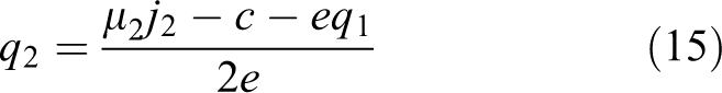
Replace q 2 with equation (15) in equation (14)

Then, the quantity of production of the first producer equals to

Likewise, applying the same procedure, the quantity of production of the second firm will equal to

Even if costs are not ignored

Total production will be

Note that since c > 0 and e < 0, Q > 0.
Let us compare equations (5) and (21).
Result I
Cournot equilibrium is total revenue maximization rather than profit maximization, even if costs are not neglected. Note that if costs are zero, then profit has already been equal to total revenue.
Multiple-plant monopoly equilibrium under a hybrid goal function
Assume that there is an owner of a multiple-plant monopoly and there are two plants. Inverse demand function is

where μ is a parameter which represents a weight that owner of the multiple-plant monopoly imposes to the manager for profit
Multiple-plant monopoly’s profit is the sum of two plants

Then, equation (22) becomes

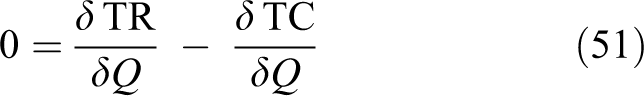
Profit is equal to the difference between total revenue (TR) and total cost (TC)


where j is average cost. Since inverse demand function is

Profit of each plant equals to


Total revenue of multiple-plant monopoly equals to


Rewrite equation (24) using equations (28), (29) and (33)

For maximization, let us take the first derivative with respect to the quantity of the first producer and equalize it to zero


Rearranging equation (36)

Leaving alone the quantity of production of the first producer
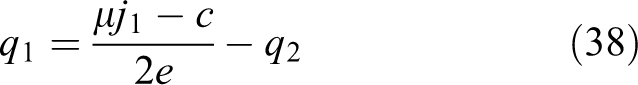
Leaving alone the quantity of production of the second producer
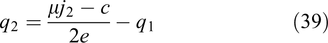
Replace q 2 with (39) in equation (38)

Rearranging equation (40)

Thus, if average costs of plants are not equal to each other as it is expected, then it should be
Result II
If average costs of plants are not equal to each other, a multiple-plant monopoly cannot maximize its profit. It should maximize its total revenue, even if costs are not zero.
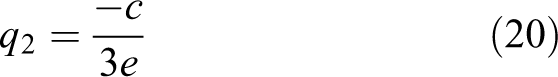
If average costs of plants are not equal to each other, and since

Thus equation (42) shows that if the objective is to maximize only total sales, then multiple-plant monopoly produces
Now assume that there is a non-multiple-plant monopoly and inverse demand function is

Total sales will be maximum when marginal revenue equals to zero

Then, rewrite equation (43) by equalizing it to zero and leaving total production alone

Note that since c > 0 and e < 0,
Result III
At equilibrium, quantity of production of a non-zero-cost multiple-plant monopoly equals to quantity of production of a total sales maximizing non-multiple-plant monopoly.
Profit maximization and producer’s equilibrium
Assume a firm’s profit is the following

where π is profit, TR is total revenue and TC is total cost.

where P is price and Q is quantity.

where w is the price of labour
Then, by replacing equation (48) with equation (46), equation (49) can be written as

If profit is maximum, then it should be

This means that it should be


where MC is marginal cost and MR is marginal revenue.
Thus, profit maximization condition is MC = MR.
Producer’s equilibrium occurs when iso-cost line is tangent to iso-quant curve which means that producer chooses labour and capital in order to minimize its cost or maximize its output. Thus, absolute value of the slope of iso-cost line
Then

or


Thus, producer’s equilibrium condition is
Then, apply maximization principle using equations (49) and (50)

Rearranging equation (57)

Dividing both sides of equation (58) by P

Since
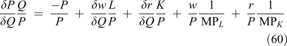
Since

One can claim that since goods and factor markets are competitive, then P, w and r do not change; they are parameters. Indeed, because of assuming perfect competition conditions, P, w and r are commonly assumed to be parameters. Note that, Stigler 48 investigates the perfect competition historically. According to him, the mathematical school is an important milestone in the building process of the concept of perfect competition. To Stigler, 48 when a mathematical economist analyses profit maximization, he first defines profit as revenue minus cost, and then, he maximizes that function. However, according to Stigler, 48 the mathematical economist encounters a situation: Revenue (or multiplication of price with quantity) varies with quantity. Thus, Stigler 48 explains that, in order to define a situation where price does not vary with quantity, perfect competition is defined where the demand curve of a firm is parallel to the quantity axis. Stigler 48 also refers to Cournot 49 and Jevons 50 in order to support that explanation. To Jevons, 50 perfect competition occurs if traders’ knowledge is perfect with regard to (i) the conditions of supply and demand and (ii) the resultant exchange ratio. Besides, to Jevons, 50 perfect competition occurs when every trader won’t exchange with any other trader upon the slightest advantage. Stigler 48 states that this definition includes single-price assumption. According to Stigler, 48 Knight 51 gives the complete formulation of the perfect competition. Knight 51 assumes an imaginary society and lists 11 characteristics of it. According to him, the first 8 of those 11 assumptions or characteristics are idealizations and for perfect competition, and those idealizations are necessary. The first thing that above-mentioned historical explanations point out is as follows: Depending on Stigler, 48 under profit maximization conditions, perfect competition is defined where the demand curve of a firm is parallel to the quantity axis in order to build a situation where price does not vary with quantity. In other words, demand curve of a firm which is parallel to the quantity axis has already been needed to explain profit maximization. However, the present study’s argument is that profit maximization does not have to be the only objective. The second consequence of above-mentioned historical explanations is as follows: Depending on Jevons, 50 perfect competition occurs with a single price such that if all agents know the resultant ratio of exchange and if each agent won’t exchange with any other agent upon the slightest advantage. In other words, the single price is needed to assume because perfect competition is a situation where there is no price advantage to firms.
Thus, assume for equation (62) that since there is perfect competition, P does not change
Thus, according to equation (62), we should assume that P, w and r depend on Q. If we assume that they do not depend on Q, a contradiction occurs as it is explained earlier with respect to equation (62). Then, whereby Stigler 48 is not wrong, how can this situation be explained? We will answer this question in the ‘Total sales maximization and economic growth’ section.
Result IV
At producer’s equilibrium conditions, assuming both factor prices and commodity prices are to be parameters includes a fallacy. We should assume that P, w and r depend on Q.
However, if we don’t assume prices are to be parameters, then stability cannot be explained. For example, if
Taking the first derivative of

Similarly, taking the first derivative of

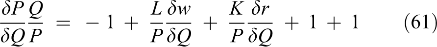
Equation (61) is rewritten by substituting

Rearranging equation (65)

Dividing and multiplying

Rearranging (67)

Equation (68) will be used. Now let us go further in the analysis by assuming Cobb–Douglas production function and constant returns to scale conditions. Note that, constant returns to scale conditions are valid in the long run

where


Equation (68) is rewritten by substituting

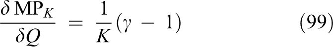
Before turning back to equation (74), now write the marginal productivity of labour using Cobb–Douglas production function

Note that, according to equation (75), we admit that
If one admits that

Since Q = K
γ
L
β and

Rearranging

Since
Thus, equation (76) will be rewritten by replacing

Rearranging


Since

Thus, if one admits that
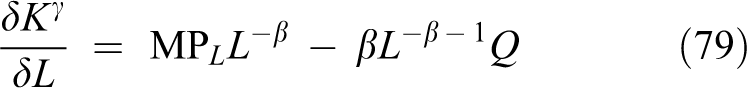
Now let us turn back to equation (75). Rearranging equation (75)

Since

Then, the first derivative of marginal productivity of labour with respect to quantity equals to

Since


Similar to the above-mentioned analysis, marginal productivity of capital equals to

Similar to equations between (76) and (85), it is admitted that
Rearranging equation (92)


Then


Now let us turn back to equation (74). Rewrite equation (74) using equations (91) and (99)
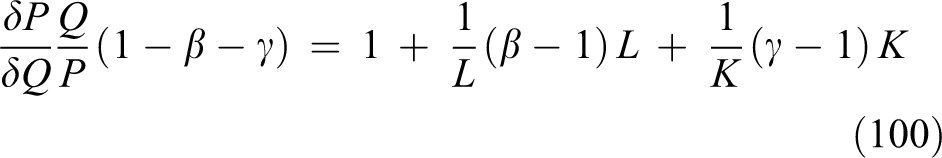


This result means that if profit is maximum (MC = MR) and if producer is at equilibrium (
One can easily show that marginal revenue (MR) is equal to zero when elasticity of quantity with respect to price is equal to −1. Marginal revenue is equal to
Dividing by P

If elasticity of quantity with respect to price is equal to −1, then

Since price has positive value, marginal revenue (MR) is equal to zero.
Result V
If profit is maximum, then it should be MC = MR = 0. If MC is positive, then profit maximization condition cannot be valid.
Total revenue maximization and producer’s equilibrium
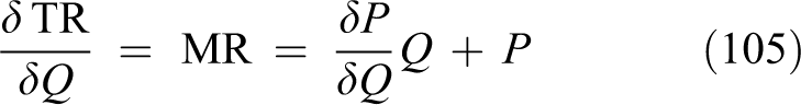
Assuming the goal as total revenue maximization, let us rewrite total revenue equation. Note that all steps will be shown for being clear

Marginal revenue is equal to

If total revenue is maximum, then

Thus, total revenue maximization condition is MR = 0. Then

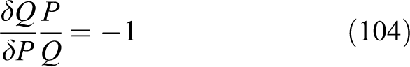
Dividing both sides of equation (102) by P

Note that, producer’s equilibrium occurs when
Rewrite equation (113) by replacing


Rearranging

Result VI
If total revenue is maximum (MR = 0) and if producer is at equilibrium (
Result VII
As a logical consequence, producer maximizes his own total revenue in all cases. Producer maximizes his profit and also total revenue, only if marginal cost is zero.
Total sales maximization and economic growth
Previous sections show that firms maximize their total sales rather than profit. This section explains the link between total sales maximization and economic growth and explains the contradiction in the section ‘Result IV’.
At first, let us explain economic growth using Figure 1. There is a negatively sloped linear demand curve and constant marginal cost in Figure 1. Recognize that economic growth occurs when the potential of the economy rises. At steady-state conditions, economic growth occurs when effective labour rises. In other words, economic growth depends on the sum of growth of labour force and growth of labour productivity. Now assume that labour productivity rises. Theoretically, since

Equilibrium at profit maximization and total sales maximization.
Assume that a firm maximizes its profit rather than total sales. Then, quantity of production and demand is equal to 0B in Figure 1. When productive capacity of the firm rises, for example, if labour productivity rises, economic growth occurs. Remember that at steady-state conditions, economic growth occurs when effective labour rises; that is, economic growth depends on the sum of labour force growth and labour productivity growth. Since
Now assume that a firm maximizes its total sales rather than profit. Then, quantity of production and demand is equal to 0A. When productive capacity of the firm rises, for example, if labour productivity rises, economic growth occurs. Since price does not depend on marginal cost, a rise in marginal productivity of labour results in an increase in wages. Note that, wages
Result VIII
Profit maximization behaviour does not have to explain economic growth. However, total sales maximization behaviour clearly explains economic growth.
These determinations also explain the contradiction in Result IV. Remember that according to Result IV, at producer’s equilibrium conditions, assuming both factor prices and commodity prices are to be parameters includes a fallacy. We should assume that P, w and r depend on Q. Again remember that, if we do not assume prices are to be parameters, the movement towards equilibrium will not have to occur. If the objective is profit maximization, then price can change. However, if the objective is total sales maximization, then there is no need to change price for producers. Price does not depend on the position of the marginal cost. This means that price depend on Q; however, there is no need to change price for producers to reach the total sales maximization objective. This solves the contradiction. Then, the last result can be written as follows.
Result IX
At producer’s equilibrium conditions, if the objective is total sales maximization, then there is no need to change price for producers to reach the total sales maximization objective. Since price does not change, moving towards equilibrium; that is, stability will have to occur under diminishing returns conditions. Total sales maximization objective, at the producer’s equilibrium conditions, guarantees stability under diminishing returns.
In the previous sections, we asked the following question: Whereby Stigler 48 is not wrong, how can this situation be explained? Remember that Stigler 48 emphasizes single price assumption for perfect competition. In other words, the single price is needed to assume because perfect competition is a situation where there is no price advantage to firms. Stigler 48 explains that, in order to define a situation where price does not vary with quantity, perfect competition is defined where the demand curve of a firm is parallel to the quantity axis. Our above-mentioned analysis shows that in order to assume a single price, one does not have to assume the firm’s demand curve as a parallel to the quantity axis when the firm’s goal is total sales maximization because at producer’s equilibrium conditions, if the objective is total sales maximization, there is no need to change price for the firms to achieve the objective of total sales maximization. Since there is no need to change price for the firms to achieve the objective, then the equilibrium price is a single price where producer’s equilibrium and total sales maximization occur and where price elasticity of demand is equal to −1.
Conclusion
This study simply investigates the objective function of a firm. The first result of the study proposes that Cournot equilibrium is total revenue maximization rather than profit maximization, even if costs are not neglected. The second result of the study shows that if average costs of plants are not equal to each other, a multiple-plant monopoly cannot maximize its profit; it should maximize its total revenue, even if costs are not zero. According to the third result of the study, at equilibrium, quantity of production of a non-zero-cost multiple-plant monopoly equals to the quantity of production of a total sales maximizing non-multiple-plant monopoly. The fourth result of the study states that at producer’s equilibrium or profit maximization conditions, assuming both factor prices and commodity prices are to be parameters includes a fallacy. One should assume that P, w and r depend on Q. The fifth result of the study shows that if profit is maximum, then it should be MC = MR = 0. If MC is positive, then profit maximization condition cannot be valid. According to the sixth result of the study, if total sales are maximum and if producer is at equilibrium, then elasticity of quantity with respect to price should be equal to −1. Note that, even if marginal cost is positive, the producer is at equilibrium and total revenue maximization condition is valid. The seventh result of the study shows that producer maximizes his own total revenue in all cases. Producer maximizes his profit and total revenue only if marginal cost is zero.
In the light of these results, it is logically proved that a firm maximizes its own total revenue or sales. In other words, profit maximization objective is only an assumption which is valid only under certain conditions.
According to the result eight, profit maximization behaviour does not have to explain economic growth. However, total sales maximization behaviour clearly explains economic growth. Note that, when total sales are maximum, price elasticity of demand will be equal to −1. This means that change in price will not have an impact on the total sales. Thus, if our argument is true, a growing economy, which grows thanks to total sales maximization behaviour of firms, should be designed where price changes do not give advantage to the firms; in other words, economic growth should occur with the help of an increase in the productive capacity of firms. Indeed, economic growth occurs when production possibility frontier shifts outward. At steady-state conditions, this can happen when effective labour rises; that is, when the sum of labour force growth and labour productivity growth rises.
Finally, the ninth result of the study points out that at producer’s equilibrium conditions, if the objective is total sales maximization, then there is no need to change price for producers to reach the total sales maximization objective. Since prices do not change, moving towards equilibrium; that is, stability will have to occur under diminishing returns conditions. Total sales maximization objective, at the producer’s equilibrium conditions, guarantees stability under diminishing returns.
Consequently, profit maximization objective is only an assumption which is valid only under certain conditions. A firm maximizes its own total revenue or sales, and economic growth occurs under total sales maximization conditions. This is the main contribution of the study. This result implies that an empirical analysis based on a strict theory should start to an analysis depending on a goal function which maximizes total sales rather than profit. Besides, this result also points out that a representative social planner who designs a growing economy, which grows thanks to total sales maximization behaviour of firms, should design that economy where price changes do not give advantage to the firms. These are the recommendations of the study.
What matters such recommendations about the practical world? How can a representative social planner or a regulative authority design an economy where price changes do not give advantage to the firms? In other words, how can a representative social planner design an economy where price elasticity of demand equals to 1? The condition where price elasticity of demand equals to 1 is closely related to the behaviour of consumers. If a firm changes its price, the quantity of demand changes because of the response of the consumers. Thus, in order to achieve economic growth, a regulative authority may impose rules or may give incentives, in order to affect behaviour of consumers for designing an economy where price changes do not give advantage to the firms. The present study recommends designing those rules or incentives as a future research subject.
Footnotes
Authors’ Note
Merter Mert is now affiliated with Department of Economics, Faculty of Economic and Administrative Sciences, Ankara Hacı Bayram Veli University, Ankara, Turkey.
Declaration of Conflicting Interests
The author(s) declared no potential conflicts of interest with respect to the research, authorship, and/or publication of this article.
Funding
The author(s) received no financial support for the research, authorship, and/or publication of this article.