A bundling strategy for items with different quality based on functions involving the minimum of two random variables

Abstract

A common strategy to increase sales and profit is to combine different types of products into bundles and sell at a discounted price. In this study, we consider the case where a wholesaler offers to sell two types of products through discount bundles. Each of the two types of products is purchased from a producer in lots that contain a percentage of imperfect quality items, which is a random variable having a known probability density function. Items received from the producer are inspected for imperfect quality using a 100% screening process. The perfect quality items are used to make the discount bundles, while the imperfect quality items are sold at a discounted price at the end of the screening period. Items of perfect quality of one type that are not bundled are kept in stock to be used in the next inventory cycle. A mathematical model is developed to determine the total profit function. A closed-form formula for the wholesaler’s optimal order quantity of each type of product is determined by maximizing the profit function. The optimal solution is given in terms of the expected values of functions involving the two random variables representing the percentages of perfect quality items. Numerical examples are provided to illustrate the model, and simulation is used to calculate the optimal solution.

Introduction

Bundling is a common marketing strategy that involves offering two or more products for sale as a single item. ¹ Companies engage in bundling strategies for many reasons. Bundles may be offered to support strategic decisions directed toward increasing the organization’s market power. Bundles can also be offered for efficiency purposes that include quality improvements, cost savings, and pricing efficiency. The growing importance for bundling of products and services is attributed to the fact that companies are establishing their strategies based on these practices. ² An empirical study conducted by Schoenherr and Mabert ³ highlighted the significance of bundling compared to other strategies.

Examples of bundling offers include a package of the same product (two tubes of toothpaste), a product and a complementary one (toothpaste and toothbrush), a product and a related one (toothpaste and liquid soap), or a product and a gift. In the service sector, bundling has been used as a differential advantage to raise customers’ interest. Restaurants offer combo meals with fries and a drink, and travel services offer flight and hotel packages. In the media sector, bundle channels are offered by cable television providers. E-tailers often combine the products with the shipping service as a bundle offer.

Bundling strategies are not implemented in the same way within industries. In general, inexpensive items are sold as a bundle, while high-end, expensive items are sold individually. Individual product demands, cost of bundling, and product category influence bundling decisions such as the optimal bundle quantity, price, and profitability. ⁴

The bundling literature has identified alternative strategies. Two of the most popular strategies are the mixed bundling and pure bundling. A firm that adopts the mixed bundling strategy chooses to sell two or more products separately or in bundles. A pure bundling strategy occurs when the firms offer to sell the entire bundle or nothing. The impacts of different bundling strategies, such as pure or mixed, for information products have been compared by Li et al. ⁵

Existing research studies addressing recent directions in the area of bundling have identified a number of factors influencing bundling decisions. Such aspects and considerations include the following: bundling in supply chain, ^6,7 product bundling in a distribution channel, ⁸ optimal composition and pricing, ² bundling of complementary products, ⁹ customized bundling, ¹⁰ and product heterogeneity and risk considerations. ¹¹ Rao et al. ¹² investigated emerging trends in product bundling by extending this concept to various new settings.

Recent literature on bundling has mainly focused on packaging discount bundles of products obtained from suppliers in lots that contain only perfect quality items. However, the assumption that items received from suppliers are all of perfect quality is rarely met in real-life situations. Very little work has been done on bundling items obtained from suppliers in lots that may contain imperfect quality items. This gap in the literature is addressed in this article. It should be noted that the common practice of bundling an imperfect quality item with a perfect one is not the strategy examined in this article. Such a strategy is often used as a marketing tool to encourage the purchase of an imperfect product. This article focuses on the case where a wholesaler acquires two types of products from two producers/suppliers. Each of the two lots contains a percentage of imperfect quality items. This percentage is a random variable having a known probability density function. The wholesaler sells bundles made of two perfect quality items of different types based on a pure bundling strategy and must decide on the optimal bundling quantity.

The rest of this article is organized as follows. In the second section, a review of related literature is presented. The mathematical model for a pure bundling strategy of two products with imperfect quality items is developed in the third section. The distribution and expected value of the minimum of two random variables are discussed in the fourth section. The calculation of the expected value of the minimum, which is needed in determining the optimal solution, is also discussed. To illustrate the model, numerical examples are provided in the fifth section. The conclusion, limitations, and suggestions for future research are given in the sixth section.

Literature review

Bundling strategies are associated with the concept of selling products with correlated demand levels in order to manage revenues and costs. Goh and Lee ¹³ refer to a bundling strategy as the selling of products jointly rather than individually and marketing them at a price different from the sum of their individual prices. Such a strategy aims at increasing the level of sales, attaining a greater market share, or outspreading the success of one product to another. ¹⁴ Consumers can benefit from a price discount if they buy the bundled products.

Two of the most popular strategies identified in the bundling literature are mixed bundling and pure bundling. A mixed bundling strategy refers to the selling of two or more products separately or in bundles. A pure bundling strategy is adopted when only bundled items are sold. Recent research studies have identified a number of factors influencing bundling decisions. The level of cooperation between suppliers within a decentralized supply chain was found to influence the bundling decisions and profitability. ⁶ Cao et al. ⁷ investigated bundling strategies driven by the limited supply of a product. The benefits of such supply-driven bundling strategy depend on the severity of supply limitation. Bhargava ⁸ considered product bundling within a distribution channel consisting of a retailer and separate manufacturers acting independently. Conflicts in the structure of the channel caused manufacturers to overprice their products, discouraging the retailers to adopt the bundling strategy.

Cataldo and Ferrer ² found that the firm’s decision related to offering multiple bundles to a single market while maintaining optimal composition and pricing strategy is influenced by consumer preferences. Yan and Bandyopadhyay ⁹ proposed a framework that enables firms to find optimum bundling product categories and pricing strategies. Their findings indicate that the value of a bundling strategy is directly proportional to the market size and price sensitivity. Hitt and Chen ¹⁰ showed that customized bundling can have a greater advantage over other bundling strategies. Sheikhzadeh and Elahi ¹¹ examined two key aspects of bundling: heterogeneity and risk considerations. They found that a risk averse decision maker is more inclined to set a bundling price lower than that of a risk neutral decision maker.

Bundles made of products provided by different firms (interfirm bundle) are effective especially when demand for bundle products is more elastic than total demand. ¹⁵ Bundling could turn into an entry barrier. In case of fierce competition, a well-established firm could resort to bundling to prevent and deter market entry of a competitor. ¹⁶ Product bundling and price bundling are different strategies. The first refers to bundles of products that provide consumers with an incremental value, while the second relates to bundles offered at a discount regardless of the goods being integrated. ¹⁷

Many marketers, at the wholesale and at the retail levels, adapt bundling strategies to increase their sales level. However, determining how to effectively and optimally make bundling decisions, especially if these products contain imperfect quality items, could prove to be very difficult. Although the literature on bundling products with imperfect quality items is scarce, research studies on inventory models, such as the classical economic order quantity (EOQ) and economic production quantity (EPQ) models with imperfect quality items, are abundant. A great deal of research has been done on incorporating factors encountered in real life into the classical EOQ and EPQ models. ¹⁸ Triggered by the work of Salameh and Jaber, ¹⁹ these classical inventory models have been recently extended in many directions to account for imperfect quality items. ^{20 –22} Salameh and Jaber ¹⁹ considered the case where each lot delivered by the supplier contains imperfect items with a known probability density function. A review of the research studies that extended, modified, or critiqued the work of Salameh and Jaber ¹⁹ can be found in Khan et al. ²³

Holt and Sherman ²⁴ discussed the effects of bundling items with uncertain quality levels on improving market efficiency. Bundling items of different qualities reduces the rejection of low-quality items. In this regard, buyers are only allowed to reject the entire bundle rather than rejecting only the least valuable item. This strategy is especially beneficial if it is impossible for sellers to resell the rejected items. To address the option of rejection, firms should consider selling bundles with reliable average quality levels. This increases sales’ efficiency since buyers are less likely to inspect and identify the quality of each unit in the bundle prior to its purchase.

Goh and Lee ¹³ studied the influence of product quality and compatibility on the consumer’s choice of bundles, particularly in the IT markets. The complementarity level or compatibility of bundled products varies in different markets, which implies that product bundles may be either complementary and functioning as a system or noncomplementary and not functioning. Such compatibility levels are determined by factors related to matching usage, derived demand, and distribution. ²⁵ Consumers are more willing to buy bundles of complementary products rather than noncomplementary ones. They perceive gaining an additional value using these products more effectively together rather than separately and by benefiting from a price discount. ²⁶ When the complementary product bundle includes a branded item, the brand image of such product would lead to higher credibility and improved customer satisfaction. ²⁷

In the following, a mathematical model is developed to describe a situation where a wholesaler is offering to sell goods only in package-form made of two types of products. The two types of products are acquired from two producers in lots that contain imperfect quality items. It is assumed that the time and cost of bundling are negligible. Items received from the producers are inspected for imperfect quality using a 100% screening process. The perfect quality items are used to make the bundles. The imperfect quality items are sold at a discounted price at the end of the screening period. Items of perfect quality of one type that are not bundled are kept in stock until the end of the inventory cycle to be used in the following inventory cycle. In this pure bundling strategy, the optimal bundling quantity is determined by maximizing the total profit per unit time function.

The mathematical model

Notation

The following notations are used:

D

bundle demand rate (units/unit time)

Q

bundle order size (units)

U_A

product A’s order size (units)

U_B

product B’s order size (units)

K_A

product A’s ordering cost (US$/unit)

K_B

product B’s ordering cost (US$/unit)

C_A

product A’s purchasing cost (US$/unit)

C_B

product B’s purchasing cost (US$/unit)

d_A

product A’s screening cost (US$/unit)

d_B

product B’s screening cost (US$/unit)

γ_A

percentage of perfect quality items of product A

f_A (γ _A )

probability density function of γ_A

γ_B

percentage rate of perfect quality items of product B

f_B (γ _B )

probability density function of γ_B

μ_A

expected value of γ_A

μ_B

expected value of γ_B

σ_A

standard deviation of γ_A

σ_B

standard deviation of γ_B

S_A

discounted selling price per unit of imperfect quality item of product A (US$/unit)

S_B

discounted selling price per unit of imperfect quality item of product B (US$/unit)

S_C

selling price per bundle (US$/unit)

x_A

product A’s screening rate (unit/unit time)

x_B

product B’s screening rate (unit/unit time)

T_A

length of product A’s screening period (unit time)

T_B

length of product B’s screening period (unit time)

T

length of the inventory cycle

h_A

product A’s holding cost (US$/unit/unit time)

h_B

product B’s holding cost (US$/unit/unit time)

TPU

total profit per unit of time

Model development

Consider the case of a wholesaler that adopts a pure bundling strategy. The wholesaler sells goods only in package-form made of two types of products, product A and product B. Let D be the demand rate of the packaged product, and let Q be the order size of packaged product per inventory cycle. A single bundle contains one unit of each type of product. The two types of products are acquired from two producers, A and B, at the beginning of the inventory cycle. Each order of type A product contains a percentage of imperfect quality items, which is a random variable γ_A having a known probability density function f_A (γ_A ). Similarly, each order of type B product contains a percentage γ_B of perfect quality items with a probability density function f_B (γ_B ). Since the order size of the bundled product is expected to be Q, the order size of the product acquired from supplier A is

$U_A=Q/{\mu }_A$

1

The expected number of perfect quality items of product A obtained from this order is exactly Q units. To prove this, let Q_A be the actual number of perfect quality items of product A found in an order received at the beginning of an inventory cycle. Then

$Q_A={\gamma }_A\hspace{0.17em}{U}_A={\gamma }_{A}Q/{\mu }_A$

2

From equations (1) and (2), the expected value of perfect quality items of product A received is

$E[Q_A\left]=E\right[{\gamma }_A{U}_A\left]=E\right[{\gamma }_A]Q/{\mu }_A={\mu }_{A}Q/{\mu }_A=Q$

3

Similarly, the order size of product B acquired from supplier B is

$U_B=Q/{\mu }_B$

4

and the actual number of perfect quality items of product B found in the order is

$Q_B\hspace{0.17em}=\hspace{0.17em}{\gamma }_B{U}_B\hspace{0.17em}={\gamma }_{B}Q/{\mu }_B$

5

From equations (4) and (5), the expected value of perfect quality items of product B received is

$E[Q_B\left]=E\right[{\gamma }_B{U}_B\left]=E\right[{\gamma }_B]Q/{\mu }_B={\mu }_{B}Q/{\mu }_B=Q$

6

Equations (3) and (6) show that the expected number of bundled items per cycle is Q. Hence, the expected inventory cycle length is

$E\left[T\right]=Q/D$

7

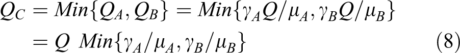
Let Q_C be the actual number of items bundled using the perfect quality items of products A and B found in the orders received from the producers at the beginning of the cycle. Then

$Q_C=Min\left\{Q_A,Q_B\right\}=Min\left\{{\gamma }_{A}Q/{\mu }_A,{\gamma }_{B}Q/{\mu }_B\right\}=QMin\left\{{\gamma }_A/{\mu }_A,{\gamma }_B/{\mu }_B\right\}$

8

which is a random variable whose probability density function is determined from the distributions of γ_A and γ_B . Define $W_A={\gamma }_A/{\mu }_A$ , $W_B={\gamma }_B/{\mu }_B$ , and

$W=Min\left\{W_A,W_B\right\}=Min\left\{{\gamma }_A/{\mu }_A,\hspace{0.17em}{\gamma }_B/{\mu }_B\right\}$

9

Let μ denote the expected value of W. From equation (8),

$E\left[Q_C\right]\hspace{0.17em}\text{= }E\left[QMin\left\{{\gamma }_A/{\mu }_A,{\gamma }_B/{\mu }_B\right\}\right]=E\left[QW\right]\text{= }QE\left[W\right]\text{=}\hspace{0.17em}Q\mu$

10

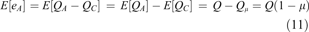
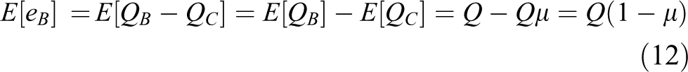
Let e_A and e_B be the excess number of perfect quality items of products A and B that are not used in bundling the packaged product. That is, e_A = Q_A − Q_C , and e_B = Q_B − Q_C . Note that at the end of the inventory cycle, e_A or e_B is zero. Moreover, the inventory cycle length is determined by the product with no unused perfect quality items (see Figure 1). From equations (3), (6), and (10),

$E\left[e_A\right]\hspace{0.17em}\text{= }E\left[Q_A-Q_C\right]\hspace{0.17em}=\hspace{0.17em}E[Q_A]-E\left[Q_C\right]\hspace{0.17em}=\hspace{0.17em}Q-Q_{\mu }=Q\left(1-\mu \right)$

11

and

$E\left[e_B\right]\text{ =}\hspace{0.17em}E\left[Q_B-Q_C\right]=E\left[Q_B\right]-E\left[Q_C\right]=Q-Q\mu =Q\left(1-\mu \right)$

12

Figure 1.

Inventory levels of types A and B products.

Hence, the average number of perfect quality items not used in bundling is the same for both types of products. Therefore, Q(1 − μ) is the expected number of on-hand inventory of perfect quality items not used in bundling the products. Hence, during each cycle, an average of Q(1 − μ) bundled items are made out of the unused perfect quality items kept in stock from the previous cycle.

Items acquired from producer A are purchased at a unit cost of C_A and an ordering cost of K_A . These items are screened for imperfect quality at a rate of x_A , where x_A > D, with a screening cost of d_A per unit. The length of the screening period is T_A = U_A /x_A . At the end of each screening period, the imperfect quality items are sold at a discounted unit selling price of S_A , where S_A < C_A . Similarly, product B is acquired at a unit purchasing cost of C_B , ordering cost of K_B , and screening cost of d_A per unit. Screening for imperfect quality items is conducted at a rate of x_B , where x_B > D, and the length of the screening period is T_B = U_B /x_B . The imperfect quality items are sold at the end of the screening period at a discounted unit selling price of S_B , where S_B < C_B . The inventory levels for both types are shown in Figure 1.

Throughout the screening period, the perfect quality items of products A and B are assumed to be bundled at a very high rate so that the package time is negligible. Also, the bundling cost is assumed to be negligible. At the end of the screening periods, the remaining inventory of perfect quality items of types A and B are bundled and used to meet the demand of the bundled products until T_C = Q_C /D. For the remainder of the inventory cycle, until time T, the excess perfect quality items from the current and previous cycles are bundled and used to meet the demand. The inventory levels of the two types of products are depicted in Figure 1.

During a typical inventory cycle, the various costs of acquiring, screening, and holding the two orders from the suppliers are as follows:

Ordering cost = K_A + K_B

Purchasing cost = C_AU_A + C_BU_B = C_AQ/μ_A + C_B Q/μ_B

Screening cost = d_AU_A + d_BU_B = d_AQ/μ_A + d_B Q/μ_B

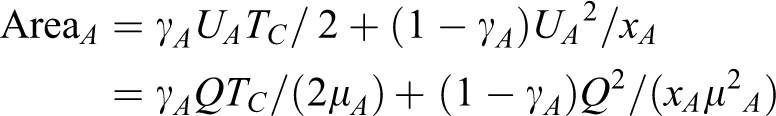
Holding cost = h_A Area _A + h_B Area _B

The two areas in the holding cost are depicted in Figure 1. That is,

${\text{Area}}_A={\gamma }_A{U}_A{T}_C/\hspace{0.17em}2+\left(1-{\gamma }_A\right)U_A{ }^2/x_A={\gamma }_{A}Q{T}_C/\left(2{\mu }_A\right)\text{\hspace{0.17em}+ }\left(1-{\gamma }_A\right)Q^2/\left(x_A{\mu }^2{ }_A\right)$

${\text{Area}}_B\hspace{0.17em}=\hspace{0.17em}{\gamma }_B{U}_B{T}_C/2+\left(1-{\gamma }_B\right)U_B{ }^2/x_B={\gamma }_{B}Q{T}_C/\left(2{\mu }_B\right)\text{+ }\left(1-{\gamma }_B\right)Q^2/\left(x_B{\mu }^2{ }_B\right)$

The revenues generated from the two orders received at the beginning of the inventory cycle are as follows:

Sales of bundles = S_C Q_C

Sales of imperfect quality items = S_A (1 − γ_A )U_A + S_B (1 − γ_B )U_B = S_A (1 − γ_A )Q/μ_A + S_B (1 − γ_B ) Q/μ_B

The total profit function per inventory cycle (TP1(Q)) resulting from the two orders received at the beginning of the inventory period is

$\text{TP}1\left(Q\right)=S_C{Q}_C+\frac{S_A\left(1-{\gamma }_A\right)Q}{{\mu }_A}+\frac{S_B\left(1-{\gamma }_B\right)Q}{{\mu }_B}-K_A-K_B-\frac{\left(C_A+d_A\right)Q}{{\mu }_A}-\frac{\left(C_B+d_B\right)Q}{{\mu }_B}-h_A\frac{Q}{{\mu }_A}\left(\frac{{\gamma }_A{T}_C}{2}+\frac{\left(1-{\gamma }_A\right)Q}{x_A{\mu }_A}\right)-h_B\frac{Q}{{\mu }_B}\left(\frac{{\gamma }_B{T}_C}{2}+\frac{\left(1-{\gamma }_B\right)Q}{x_B{\mu }_B}\right)$

13

In addition to TP1(Q), the excess perfect quality items from the current and previous cycles are bundled and sold resulting in a total profit TP2(Q). This function is the revenue obtained from selling the items bundled using the excess good-quality items minus the holding cost of the excess items. Hence, the total profit per cycle TP(Q) = TP1(Q) + TP2(Q). The total profit per unit time function is

$\text{TPU}\left(Q\right)=\text{TP}\left(Q\right)/T=(\text{TP}1\left(Q\right)+\text{TP}2\left(Q\right))/T$

14

By the renewal reward theorem, ²⁸

$E\left[\text{TPU}\left(Q\right)\right]=E\left[\text{TP}\left(Q\right)\right]/E\left[T\right]=E\left[\text{TP}1\left(Q\right)+\text{TP}2\left(Q\right)\right]/E\left[T\right]=E\left[\text{TP}1\left(Q\right)\right]/E\left[T\right]+E\left[\text{TP}2\left(Q\right)\right]/E\left[T\right]$

15

From equation (13), the expected average excess of each type of product E[e_A ] and E[e_B ] is equal to Q(1 − μ). Hence, the expected number of bundled items obtained from the excess is also Q(1 − μ). Accordingly,

$E\left[\text{TP}2\left(Q\right)\right]=S_{C}Q\left(1-\mu \right)-h_A\left(1-\mu \right)QT-h_B\left(1-\mu \right)QT$

16

Also,

$E\left[TP1\left(Q\right)\right]=S_{C}Q\mu +\frac{S_A\left(1-{\mu }_A\right)Q}{{\mu }_A}+\frac{S_B\left(1-{\mu }_B\right)Q}{{\mu }_B}-K_A-K_B-\frac{\left(C_A+d_A\right)Q}{{\mu }_A}-\frac{\left(C_B+d_B\right)Q}{{\mu }_B}-h_A\frac{Q}{{\mu }_A}\left(\frac{E\left[{\gamma }_A{T}_C\right]}{2}+\frac{\left(1-{\mu }_A\right)Q}{x_A{\mu }_A}\right)-h_B\frac{Q}{{\mu }_B}\left(\frac{E[{\gamma }_B{T}_{C }]}{2}+\frac{\left(1-{\mu }_B\right)Q}{x_B{\mu }_B}\right)$

17

Therefore, equations (16) and (17) give that the expected total inventory profit per cycle is

$E\left[\text{TP}\left(Q\right)\right]=S_{C}Q+\frac{S_A\left(1-{\mu }_A\right)Q}{{\mu }_A}+\frac{S_B\left(1-{\mu }_B\right)Q}{{\mu }_B}-K_A-K_B-\frac{\left(C_A+d_A\right)Q}{{\mu }_A}-\frac{\left(C_B+d_B\right)Q}{{\mu }_B}-h_A\frac{Q}{{\mu }_A}\left(\frac{QE\left[{\gamma }_{A}W\right]}{2D}+\frac{\left(1-{\mu }_A\right)Q}{x_A{\mu }_A}\right)-h_B\frac{Q}{{\mu }_B}\left(\frac{QE[{\gamma }_{B}W]}{2D}+\frac{\left(1-{\mu }_B\right)Q}{x_B{\mu }_B}\right)-h_A\left(1-\mu \right)QT-h_B\left(1-\mu \right)QT$

18

Using equations (15) and (18), the expected total inventory profit per unit time function is

$\text{ETPU}\left(Q\right)=S_{C}D+S_{A}D\left(\frac{1-{\mu }_A}{{\mu }_A}\right)+S_{B}D\left(\frac{1-{\mu }_B}{{\mu }_B}\right)-\frac{\left(K_A+K_B\right)D}{Q}-\frac{D\left(C_A+d_A\right)}{{\mu }_A}-\frac{D\left(C_B+d_B\right)}{{\mu }_B}-Q\left(1-\mu \right)\left(h_A+h_B\right)-h_A\frac{D}{{\mu }_A}\left(\frac{QE\left[{\gamma }_{A}W\right]}{2D}+\frac{\left(1-{\mu }_A\right)Q}{x_A{\mu }_A}\right)-h_B\frac{D}{{\mu }_B}\left(\frac{QE[{\gamma }_{B}W]}{2D}+\frac{\left(1-{\mu }_B\right)Q}{x_B{\mu }_B}\right)$

19

Differentiating the expression of ETPU(Q) in equation (19) with respect to Q gives

$\frac{\mathit{\text{dETPU}}}{\text{d}Q}=\frac{\left(K_A+K_B\right)D}{Q^2}-\left(1-\mu \right)\left(h_A+h_B\right)-h_A\left(\frac{E\left[{\gamma }_{A}W\right]}{2{\mu }_A}+\frac{D\left(1-{\mu }_A\right)}{x_A{\mu }_A^2}\right)-h_B\left(\frac{E\left[{\gamma }_{B}W\right]}{2{\mu }_B}+\frac{D\left(1-{\mu }_B\right)}{x_B{\mu }_B^2}\right)$

20

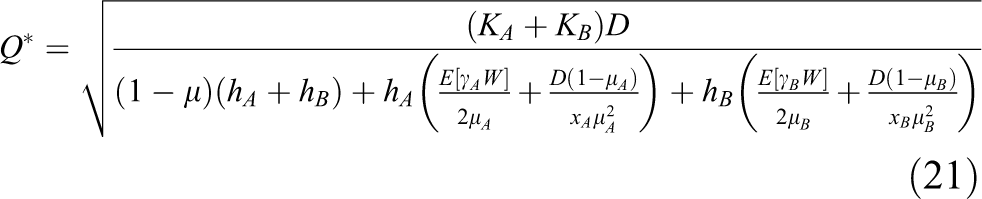
Setting the derivative in equation (20) equal to zero and solving for y, the optimal order quantity is obtained as

$Q^{*}=\sqrt{\frac{\left(K_A+K_B\right)D}{\left(1-\mu \right)\left(h_A+h_B\right)+h_A\left(\frac{E\left[{\gamma }_{A}W\right]}{2{\mu }_A}+\frac{D\left(1-{\mu }_A\right)}{x_A{\mu }_A^2}\right)+h_B\left(\frac{E\left[{\gamma }_{B}W\right]}{2{\mu }_B}+\frac{D\left(1-{\mu }_B\right)}{x_B{\mu }_B^2}\right)}}$

21

Note that the optimal order quantity is the unique maximizer since the second derivative of the TPU function is

$\frac{d^{2}ETPU}{d{Q}^2}=-\frac{2\left(K_A+K_B\right)D}{Q^3}$

which is always negative.

Note that the optimal solution is given in terms of the expected value μ of the random variable W, which is the minimum of the random variables W_A =  γ_A/μ_A and W_B =  γ_B/μ _B . The following section discusses how μ can be calculated.

The distribution and expected value of the minimum of a set of random variables

The general case

Given the two independent random variables γ_A and γ_B , with known probability density functions f_A (γ_A ) and f_B (γ_B ), consider the random variables W_A =  γ_A/μ_A and W_B =  γ_B/μ_B , where μ_A and μ_B are the expected values of γ_A and γ_B , respectively. The probability density function g_A (w_A ) and g_B (w_B ) of W_A and W_B are obtained from f_A (γ_A ) and f_B (γ_B ). Since γ_A and γ_B are independent, the random variables W_A and W_B are also independent. Moreover, the expected values of the random variables W_A and W_B are both equal to 1, and the variances are equal to ${\sigma }_A^2/{\mu }_A^2$ and ${\sigma }_B^2/{\mu }_B^2$ , respectively. Let the random variable W be defined as W = Min{W_A , W_B }. The cumulative distribution of W is given by

$G\left(t\right)=Prob\left(W\le t\right)=\int {\int }_R\gamma \left(w_A,w_B\right)d{w}_{A}d{w}_B$

where the region R is the intersection between the domain of g(w_A , w_B ) and the complement of a rectangular region representing W ≤ t. Given the fact that W_A and W_B are independent, the cumulative distribution of W becomes

$G\left(t\right)=Prob\left(W\le t\right)=1-\left(\underset{t}{\overset{\infty }{\int }}{g}_A\left(w_A\right)d{w}_A\right)\left(\underset{t}{\overset{\infty }{\int }}{g}_B\left(w_B\right)d{w}_B\right)=1-G_A\left(t\right)G_B\left(t\right)$

22

which is the complement of the product of the complementary cumulative distributions G_A (t) and G_B (t) of W_A and W_B . Once the cumulative distribution G(t) is determined, the probability density function g(t) can be obtained by differentiating G(t). That is,

$g\left(t\right)=-{G\prime }_A\left(t\right)G_B\left(t\right)-G_A\left(t\right){G\prime }_B\left(t\right)$

23

The expected value of W is then obtained by $E\left(W\right)=\underset{-\infty }{\overset{\infty }{\int }}t\hspace{0.17em}g\left(t\right)\hspace{0.17em}dt$ .

The case where W_A and W_B are uniformly distributed is presented next.

The uniform distribution case

Consider the case where γ_A and γ_B are uniformly distributed over [a, b] and [c, d], respectively. Then, f_A (γ _A ) = 1/(b − a) whenever a < γ _A < b, and f_A (γ_A ) = 0 otherwise. Moreover, μ_A = E[γ_A ] = (a + b)/2. Similarly, f_B (γ_B ) = 1/(d − c) whenever c < γ _B < d, and f_B (γ_B ) = 0 otherwise. Also, μ_B = E[γ_B ] = (c + d)/2. Then, W_A = γ_A /μ_A is uniformly distributed over [a/μ_A , b/μ_A ], and E[W_A ] = 1. Since E[W_A ] = 1 is the midpoint of the interval [a/μ_A , b/μ_A ], this interval can be represented as [1 − m_A , 1 + m_A ], where m_A = (b − a)/(a + b), and the probability density function of W_A is given by

$g_A\left({\gamma }_A\right)=\{\begin{array}{ccc}\frac{1}{2m_A}& \text{if}& 1-m_A<{\gamma }_A<1+m_A\\ 0& & \text{otherwise}\end{array}$

24

Also, the complement cumulative probability function is given by

$G_A\left(t\right)=\{\begin{array}{ccc}1& \text{if}& t\le m_A\\ \frac{1+m_A-t}{2m_A}& \text{if}& 1-m_A<t<1+m_A\\ 0& \text{if}& t\ge 1+m_A\end{array}$

25

Similarly,

$G_B\left(t\right)=\{\begin{array}{ccc}1& \text{if}& t\le m_B\\ \frac{1+m_B-t}{2m_B}& \text{if}& 1-m_B<t<1+m_B\\ 0& \text{if}& t\ge 1+m_B\end{array}$

26

To find the cumulative distribution G(t) of the random variable W, G_A (t)·G_B (t) is determined by assuming that m_A ≤ m_B . Hence, the intervals [1 − m_A , 1 + m_A ] ⊆ [1 − m_B , 1 + m_B ] so that

$1-m_B\le 1-m_A\le 1\le 1+m_A\le 1+m_B$

Note that when t ≥ 1 + m_A , G_A (t) = 0, and the product G_A (t)·G_B (t) is 0. If 1 − m_A ≤ t ≤ 1 + m_A , then G_A (t) = (1 + m_A − t)/2m_A and G_B (t) = (1 + m_B − t)/2m_B . When 1 − m_B ≤ t ≤ 1 − m_A , G_A (t) = 1 and G_B (t) = (1 + m_B − t)/2m_B . Hence,

$G\left(t\right)=\hspace{0.17em}\{\begin{array}{l}\hspace{1em}\hspace{1em}0\hspace{1em}\hspace{1em}\hspace{1em}\hspace{1em}\hspace{1em}\hspace{1em}\hspace{1em}\hspace{1em}\hspace{1em}\text{if}\hspace{1em}\hspace{1em}t\le 1-m_B\\ \hspace{0.17em}\hspace{0.17em}\hspace{0.17em}\hspace{0.17em}\hspace{0.17em}\hspace{0.17em}\hspace{0.17em}\left(t+m_B-1\right)/\left(2m_B\right)\hspace{0.17em}\hspace{0.17em}\hspace{0.17em}\hspace{0.17em}\hspace{0.17em}\hspace{0.17em}\hspace{0.17em}\hspace{1em}\hspace{1em}\text{if}\hspace{0.17em}\hspace{0.17em}\hspace{0.17em}\hspace{0.17em}\hspace{0.17em}\hspace{0.17em}\hspace{0.17em}1-m_B\le t\le 1-m_A\\ 1-\frac{\left(1+m_A-t\right)\left(1+m_B-t\right)}{4m_A{m}_B} \text{if} 1-m_A\le t\le 1+m_A\\ \hspace{1em}\hspace{1em}1\hspace{1em}\hspace{1em}\hspace{1em}\hspace{1em}\hspace{1em}\hspace{1em}\hspace{1em}\hspace{1em}\hspace{1em}\text{if}\hspace{1em}\hspace{1em}t\ge 1+m_A\end{array}$

27

The probability density function g(t) of W is obtained by differentiating equation (27). The expected value E(W) is then calculated by E[W] = ∫t g(t) dt. Therefore,

$E\left[W\right]=\mu =1-\hspace{0.17em}\hspace{0.17em}\frac{m_A^2+3m_B^2}{12\hspace{0.17em}{m}_B}$

28

Hence,

$E\left[Q_C\right] =Q_{\mu }=Q\left(1-\frac{m_A^2+3m_B^2}{12\hspace{0.17em}{m}_B}\right)$

29

and

$E\left[e_A\right]\hspace{0.17em}\text{=}\hspace{0.17em}\text{E}\left[e_B\right]\hspace{0.17em}= \hspace{0.17em}Q\left(\frac{m_A^2+3\hspace{0.17em}{m}_B^2}{12\hspace{0.17em}{m}_B}\right)$

30

Note that the calculation of the expected values E[γ_AW] and E[γ_AW] appearing in the expression of the optimal solution Q* is beyond the scope of this study. These values are determined via simulation as illustrated in the numerical example below.

Numerical example

Suppose that the demand rate for the packaged product is 200 bundles per day. A single item of each of the two types of products, A and B, is packaged to form a single bundle. Suppose that the ordering cost for product A is US$282 and for product B is US$300. The unit purchasing costs for products A and B are US$2 and US$3, respectively. The screening rate for imperfect quality items of product A is 400 units/day and 600 units/day for product B. The percentage of perfect quality items is uniformly distributed over [70%, 90%] for product A and [65%, 85%] for product B. The screening cost per unit is US$0.1 for product A and US$0.2 for product B. The holding cost per unit is US$0.01 for product A and US$0.15 for product B. Imperfect items can be sold at a discounted price of US$1 for product A and US$2 for product B. Packaged items can be sold at a price of US$10 per bundle. The holding cost is US$0.01 per unit per day for product A and US$0.02 per unit per day for product B. Therefore, the parameters in this case are as follows:

D = 200 units/day, K_A = US$282; K_B = US$300, x_A = 400 units/day, x_B = 600 units/day, a = 0.70, b = 0.90, c = 0.65, d = 0.85; C_A =US$2/unit, C_B = US$3/unit, d_A = US$0.1/unit, d_B = US$0.15/unit, S_A = US$1/unit, S_B = US$2/unit, S = US$10/unit, h_A = US$0.01/unit/day, and h_B = US$0.02/unit/day.

Substituting the values of the parameters in expression (21), the optimal order quantity Q* for the packaged product is found to be 2401.53 units. Since TPU(2401.53) = TPU(24000) = US$721.33, we set Q*= 2400 units. Hence, the expected inventory period E[T] = Q/D = 12 days, and the expected time to sell items using the orders received at the start of period is E[T_C ] = Q_C/D = 11.48 days. Since the percentage of imperfect items of product A is uniformly distributed over [70%, 90%], we have μ_A = 80% and the order size of product A is U_A = Q/μ_A = 3000 units, and the screening period T_A = U_A /x_A = 7.5 days. The procurement and screening cost per cycle is K_A + (C_A + d_A ) U_A − S_A (1 − μ _A ) U_A = US$282 + (US$2 + US$0.1) 3000 − US$1 (1 − 0.8) 3000 = US$5982. As for product B, μ_B = 75%, the order size is U_B = Q/μ_B = 3200 units, and the screening period T_B = U_B /x_B = 5.33 days. The procurement and screening costs per cycle for product B is US$300 + (US$3 + US$0.15) 3200 − US$2 (1 − 0.75) 3200 = US$8780.

To calculate the holding cost, one needs to determine E[Q_C ] = μQ and E[e_A ] = E[e_B ] = Q(1 − μ), where Q_C = Min{Q_A = Qγ_A /μ_A , Q_B = Qγ_B /μ_B }. Now W_A = γ_A /μ_A is uniformly distributed over [0.875, 1.125] so that m_A = 0.125 and g_A (w_A ) = 1/(2m_A ) = 4. Similarly, W_B = γ_B /μ_B is uniformly distributed over [0.867, 1.133], m_B = 0.133, and g_B (w_B ) = 1/(2m_B ) = 3.76. From equation (28), W = Min {W_A , W_B } has an expected value of E[W] = μ = 0.9569. Therefore, E[Q_C ] = μQ = 2297 units and E[e_A ] = E[e_B ] = 103 units. The behavior of the profit function is depicted in Figure 2.

Figure 2.

Total profit function.

Note that when n ≥ 3 or when the distributions are not uniform, the expected value μ of W may be obtained by a numerical calculation or by simulation.

Conclusion

This article investigated the influence of the quality of items used in a pure bundling strategy. The case where a wholesaler sells goods only in packaged form made of two types of products was examined. The two types of products are acquired from two producers/suppliers in lots each of which contains a percentage of imperfect quality items. The percentage of imperfect quality items of each type is a random variable having a known probability density function. A mathematical model for this pure bundling strategy was developed and used to derive the wholesaler’s optimal bundling quantity. Based on maximizing the total profit function, a closed-form formula for the optimal bundling quantity was obtained. The formula contains expected values of functions of random variables related to the percentages of imperfect quality items. The calculations of these expected values and the optimal solution were completely described. Determining the optimal bundling quantity when the cost, revenue, and quality parameters of the two types of products are considered simultaneously addresses a gap in the bundling research. A numerical example was provided to illustrate the calculations of the expected values needed in determining the optimal bundling quantity. Furthermore, the calculations of the various cost and revenue components were also illustrated. The findings demonstrated by the analytical solution and illustrated by the numerical example offer key managerial implications.

From a managerial perspective, the findings can help managers identify the appropriate quantities ordered from the different suppliers and the corresponding optimal bundling quantity that yields a maximum profit. Moreover, managers can use the proposed model to develop their marketing strategies. The findings suggest that, in the presence of imperfect quality items, deciding on the order size to be acquired from each of the two suppliers should not be done separately. This decision must be made according to the modeling approach followed in this article, which considers the cost, revenue, and quality parameters of the two types of products simultaneously.

The adoption of a pure bundling strategy and the development of the model based on two products are limitations of this study. Using simulation to calculate expected values needed for the calculation of the optimal bundling quality is another limitation.

This model can be extended and generalized in many directions to incorporate factors encountered in real-life situations. For instance, the problem can be modeled in the supply chain context. In another direction, we suggest that the model be extended to a mixed bundling strategy. Also, a model with more than two products can be considered.