Optimizing the integrated production and maintenance planning using genetic algorithm

Abstract

In spite of the interdependence between them, production and maintenance planning decisions are generally studied and used independently in the majority of the manufacturing systems. Our contribution is summarized to obtain a maintenance policy including preventive replacement in each maintenance cycle and minimal repair in case of unplanned failure, and on the other side, for a set of products and in each period, specify the quantity to be produced and when is the production set up, also the stock and the breaking on demand level, so that to minimize the total cost. The purpose of the research was aimed at achieving the optimization of an integrated planning of preventive maintenance and production in a multi-period, multiproduct, and single-line production system. To achieve this purpose, our model is configured as a mixed integer linear programming and solved by IBM ILOG CPLEX OPL studio 12.6 (USA), and we propose our own genetic algorithms (GAs) using Python solver with respect to resolution time and the quality of results. Then, to find the performance of the model and the usefulness of the proposed resolution method, a numerical example is considered to produce two products for a finite horizon with 11 periods. The results of the analysis show that this GA provides a new tool for the integrated planning in the industrial sector. These results reflect the experiences of single-line system and further studies are needed for generalizability in the multiline cases, also we will compare the proposed GA with other evolutionary algorithms.

Introduction

The operation of production systems has become increasingly complex and the maintenance process has intensified by insisting on an efficient planning of maintenance. Our contribution aims to anticipate if we should do a minimal repair action or prevent a periodic replacement and to define the quantities to be produced, the stock level, and the case of the breaking on demands per period and product. However, the complexity of the production requires a heuristic to solve the problem. In this article, an integrated planning is proposed to satisfy the customer demands while respecting the cost, quality, and delay. We can find many research linked to the integrated production and maintenance planning in the literature by Ettaye et al. ¹ during the recent years.

The first research that establishes a really integrated planning is that of Aghezzaf et al. It considered the unplanned production failure, preventive and corrective maintenance actions, by acting on the availability and therefore the current system capacity in every period for multi-products single machine system. In its resolution, they used the CPLEX solver for the mixed integer linear problem without considering the breaking on demand case. ² The work of Aghezzaf et al. ³ considered integrated planning problem in the case of a set of parallel production lines such as extension of the previous work and they resolve their model with a Lagrangian relaxation method. In their model, ⁴ Ben Ali et al. solve the production problem by applying an elitist genetic algorithm (GA) subject to periodic preventive replacement so as to minimize the makespan and the production costs. The approach used by Nourelfath et al. ⁵ integrated the tactical production planning with the periodic preventive maintenance of a multistate system by minimizing the total cost of the two functions; an exhaustive evaluation was handled to resolve the proposed model, but it can only deal with the problems of small size. Concerning the multistate systems, the authors utilize a GA. The simulated annealing method was exploited by Fitouhi and Nourelfath ⁶ who extended the previous model to meet the nonperiodic situation. On the other side, the model by Yalaoui et al. ⁷ has taken into consideration the degradation of production line in case of multiproducts, has multi-periods and multilines, and this deterioration is modeled with the production lines capacity reduction in each period of time, for a small system they solved the problem with a linear relaxation method and for the complex systems the fix and relax method was useful. In another context, taking into consideration the capacity and the system reliability, Najid et al. ⁸ proposed a joint production and maintenance planning model subject to random failure; they also used a time windows approach to minimize the demand shortage in case of high demand and to give more flexibility for preventive replacement. They used optimization with the XPRESS solver for small problems and for larger problems the GA. After that, Ettaye et al. ⁹ modified the model of Aghezzaf et al. ² by adding the constraint of breaking on demand and set up time criterion and solved the mixed integer linear problem with MATLAB solver 2016b (optimization toolbox: intlinprog function as a Mixed-integer linear programming solver). In case of the multilines problem, Ettaye et al. ¹⁰ has extended the previous model and used integrated linear programming of the CPLEX solver. Then, Beheshti-Fakher et al. ¹¹ proposes a hybrid GA with tabu search method for an integrated planning of imperfect production systems.

The integrated planning model

The production planning, in the field of industry, does not take into account unscheduled stops and the maintenance activities are considered as a perturbation in the production process. This conflict of interest between the two departments can be summarized by the mutual non-consideration of the requirements and the needs of these two vital operations in a production system, and then the lack of synchronization makes the problem more complex. To resolve this problem, we propose an integrated planning that aims to minimize the total cost which contains production, storage, breaking on the demand, preventive replacement and minimal repair costs.

The total maintenance cost

We consider a finite planning horizon with a degraded component of our used system. Knowing that this degradation augments the failure rate and decreases the system reliability and availability, the lifetime of production line follows a probability distribution, either gamma or Weibull law, and the failure rate is defined by the following equation

${\displaystyle {\int }_0^{\Delta }\lambda (t)\text{\hspace{0.17em}d}t}={\displaystyle {\int }_0^{\Delta }\frac{f(t)}{1-F(t)}\text{d}t}=\text{log}\left(\frac{1-F(0)}{1-F(\Delta )}\right)=-\text{log}(1-F(\Delta ))\text{with\hspace{0.17em}}F(0)=0$

1

where λ is the failure rate, f is the probability density function, and F is the cumulative distribution function.

For this reason, we are forced to propose a maintenance policy that deals with this kind of problem. In effect, our policy proposes to do a preventive replacement for each maintenance cycle beginning, except the first period of the horizon and to do a minimal repair in the situation of aleatory failure inside the maintenance cycle (corrective maintenance). Hence the importance of calculating the total maintenance cost is established in equation (2). According to the calculations made by Yalaoui et al. ⁷ and Ettaye et al., ⁹ the cost becomes as defined by the following equations

$\text{CM}(k)=\frac{N}{k}\left(C_p+C_c{\displaystyle {\int }_0^T\lambda (t)\text{\hspace{0.17em}d}}t\right)\forall t\in H$

2

$\text{CM}(k)=\left(\left[N/k\right]\times C_p\right)-\left(C_c\times \text{log}\left[{(1-F(k\times \tau ))}^{\left[N/n1\right]}\times (1-F((N-\left[N/k\right]k)\times \tau ))\right]\right)\text{with\hspace{0.05em}\hspace{0.05em}\hspace{0.05em}\hspace{0.05em}\hspace{0.05em}\hspace{0.05em}\hspace{0.05em}}T=k\times \tau$

3

where CM is the total maintenance cost, N is the number of periods, k is the number of periods in the maintenance cycle, C_p is the preventive replacement cost $C_p\le C_c$ ,C_c is the minimal repair cost, λ is the failure rate, H is the planning horizon,tis the basis period, and T is the cycle of preventive replacement.

The available capacity

Knowing that each production system has its own maximal capacity C _max and each maintenance activity consumes a percentage of this capacity ( $P_p=a\times C_{\text{max}}\text{ and }{P}_c=b\times C_{\text{max}}$ ), the available capacity for each period t is done in units of time by the relation below based on the calculations made by Yalaoui et al. ⁷ and the relation (1).

$C(t)=\{\begin{array}{l}C(\tau )=C_{\text{max}}-Pp+(Pc\times \text{\hspace{0.17em}log}(1-F(\tau )))\text{\hspace{0.17em}\hspace{0.17em}\hspace{0.17em}if\hspace{0.17em}\hspace{0.17em}}n=1\\ C(n\tau )=C_{\text{max}}-(Pc\times (\text{log}(1-F((n-1)\times \tau ))-\text{log}(1-F(n\times \tau ))))\text{\hspace{0.05em}\hspace{0.05em}with\hspace{0.05em}\hspace{0.05em}\hspace{0.05em}}(n=2,\mathrm{...},k-1)\\ C(t)=C(u\tau )\text{\hspace{0.17em}\hspace{0.17em}with\hspace{0.17em}\hspace{0.17em}}(t=kq\tau +u\tau );\\ \text{with\hspace{0.05em}\hspace{0.05em}\hspace{0.05em}}q\in \left\{1,\mathrm{...},\left[N/k\right]\right\};u\le (k-1)\times \tau ;u\le N-qk\tau \end{array}$

4

where C is the available capacity during the period t, C _max is the maximal capacity, F is the cumulative distribution function, P_p is the capacity consumption for preventive replacement, P_c is the capacity consumption for minimal repair, N is the number of periods, C_p is the preventive replacement cost, C_c is the minimal repair cost, and T is the cycle of preventive replacement.

The total production cost

To express the production cost, we based on multi-periods and multiproducts, capacitated the lot sizing problem, then we added the breaking on the demand constraints and the setup time criterion. From the summation of the launching costs, the production, storage, and breaking on the demand costs, we deduce the total production cost by

$\text{CP}(k)={\displaystyle \sum _{i=1}^{\text{NR}}{\displaystyle \sum _{t=1}^N\left({\alpha }_{it}{x}_{it}+{\beta }_{it}{y}_{it}+{\gamma }_{it}{s}_{it}+{\phi }_{it}{r}_{it}\right)}}\forall i\in R\forall t\in H$

5

where CP is the total production cost, NR is the number of products, N is the number of periods, α_it is the production cost of the product i in the product t, x_it is the quantity to be produced of the product i in the period t, β_it is the launching cost, y_it is the launching variable, γ _it is the storage cost, s_it is storage level, φ_it is the breaking on the demand cost, r_it is the breaking on the demand level, and R is the set of references.

Model formulation

To define our model, we have represented the proposed planning in Figure 1 which contains the maintenance activities and its times and the capacities of each period.

Figure 1.

The integrated planning.

The main objective of our integration is to reduce the total cost of production and maintenance, since the maintenance cost is very small compared to the one of the production, we apply the optimization by GA method at the level of the lot sizing problem with finite capacity and setup time. Based on the minimal production cost, we deduce the optimal planning.

On the other side, the objective function of our suggested model minimizes the total cost that contains the production planning (producing, launching, storage, and breaking on demand costs) and the maintenance plan (preventive and corrective actions costs) as defined by equation (6), subject to a set of constraints given by:

$\text{min}\left({\displaystyle \sum _{i=1}^{\text{NR}}{\displaystyle \sum _{t=1}^N\left({\alpha }_{it}{x}_{it}+{\beta }_{it}{y}_{it}+{\gamma }_{it}{s}_{it}+{\phi }_{it}{r}_{it}\right)}}+\text{CM}(k)\right)$

6

Subject to

$xit+rit-sit+si(t-1)=dit;\forall i\in R\forall t\in H$

7

where d_it is the demand

${\displaystyle \sum _{i=1}^{\text{NR}}\left(v_{it}{x}_{it}+f_{it}{y}_{it}\right)}\le C(t);\forall t\in H$

8

where v_it is the variable resources need (processing time) and f_it is the fixed resources need (setup time)

$x_{it}\le M_{it}*y_{it};\forall i\in R\forall t\in H$

9

where M is the production upper bound

$r_{it}\le d_{it};\forall i\in R\forall t\in H$

10

$x_{it},s_{it},r_{it}\ge 0;\forall i\in R\forall t\in H$

11

$y_{it}\in \left\{0,1\right\};\forall i\in R\forall t\in H$

12

$s_{i0}=0;\forall i\in R$

13

• Relation (7) indicates the flows conservation through the planning horizon for the product i in the period t, it reflects that the available stock of the product i increases with the produced quantity to satisfy the demand in the actual period and the rest is stored for ulterior periods as a penury.

• Relation (8) shows that the planning that we want to have must be with a limited capacity. In fact, for realizing a plan, we have a quantity of resources that will be consumed during the production of each product. The total summation must be less than the available capacity C(t), which is done in every period t using the relation (4).

• Relation (9) reflects the fact that if there is a production installation, so the quantity to produce must be less than production upper bound (14). This value is given by the minimum of the maximum quantity of product which can be produced and the available demand on a segment of the horizon $[t,\mathrm{...},{\lambda }_{it}]$ .

  $M_{it}\text{=min}\left\{{\displaystyle \sum _{t\text{'}=t}^{{\lambda }_{it}=N\times \tau }{d}_{it\text{'}};((C(t)-f_{it})/{\nu }_{it})}\right\};\forall i\in R\forall t\in T$

  14

• Relation (10) assures that the breaking on demand level is less than the demand for product i by the end of period t.

• Relation (11) ensures that the variables x_it , s_it, and r_it are continuous positive.

• Relation (12) shows the fact that y_it is a dependent binary variable of production for the product i and the period t.

• Finally in relation (13), the initial stock is void at t = 0.

Resolution method

To determine the optimal production and maintenance integrated planning for our proposed model, we used the following procedure:

For k = 1,…, N:

Evaluate the total maintenance cost CM(k) (in this case, the optimal cycle (T* = k × τ) is the one coinciding with the minimal value of CM(k*)).

Evaluate the capacity values C(t, k).

Use the genetic algorithm program with Python to solve the multiproducts capacitated lot sizing problem with setup time and breaking on demand constraint, so that to determine the production cost CP(k) using the capacity obtained.

Deduce the overall cost C _total(k) and select the optimal cycle T*, which is equivalent to min {C _total(k)}.

End For

Deduct the solution by giving T and the arrays x, y, s, r.

All numerical works have been made in a computer with microprocessor core i5, 5th generation and 4GB of RAM. Then we code the solution algorithm using MATLAB R2016b and Python 3.4.4.2 solvers.

Genetic algorithm principle

GAs are defined as a heuristic optimization inspired by the natural evolution. This method has been applied successfully in its application to a large group of real industrial problems with important complexity using the nature. GA begins with initial population constructed from a set of random chromosomes. Each individual from the population is named a chromosome which evolves through successive generations called iterations. In each generation, the fitness is calculated to evaluate the chromosomes. Then, the crossover and the mutation operations are performed in order to create the following generation. However, some elements in the new generation are replaced by new random chromosomes in the evaluation operator, so that to conserve the population size constant. After a certain number of generations, the solution converges toward the best optimal solution. The basic concept of the GA used in our article can be represented in the Figure 2, and the algorithm procedure is shown in the next paragraph.

Figure 2.

Genetic algorithm principle.

Genetic algorithm procedure

Begin generational GA

ite = 0

Produce initial population by a random initialization respecting all of the model constraints P(ite).

Evaluate the fitness values of members in P(ite) and deduce the minimum of f_obj0.

Select and class the values of f_obj0 using Stochastic sampling with replacement method and deduce the minimum of f_obj1 after selection and produce new P(ite).

While ite < max_ite do:

Select two parents.

Using the selected parents P(ite-1) and the crossover operator with the probability pcmake offsprings.

Using the mutation operator with the probability pm Mutate the offsprings in P(ite-1).

Calculate the fitness values of members in P(ite).

Do a filtering of the obtained fitness and deduct the minimum of f_obj(ite) for each ite.

ite + 1

end while

Compare min_f_obj0, min_f_obj1, min_f_obj(ite).

End generational GA

Population initialization

As shown in the step (1) of the procedure, the GA must have an initial population. The most common standard method is to generate solutions randomly for the full population. However, by respecting the boundary constraints, since GAs can iteratively improve existing solutions, the starting population can be produced with powerful solutions.

Concerning the coding of the decision variables, each chromosome is composed of four parts defining the different production costs with the dimension: [number of products × number of periods] (see Figure 3).

Figure 3.

Chromosome representation.

Evaluation and selection operator

The operators of reproduction are applied to emphasize the best solutions and remove bad solutions in the population, while keeping the population size unchangeable. There are several kinds of reproduction operators; the rank order selection is one of the famous methods where the best chromosomes are selected for the feasible population.

A stochastic sampling selection process with replacement is adopted for our proposed GA in which a population element can be selected more than one time. It is proposed to be the standard selection method in programming with GA, mainly because it is generally accepted as a multifunctional technique that has been broadly implemented. Moreover, this method has also found relevance in a variety of areas.

Also named as roulette wheel selection, the stochastic sampling with replacement method says that the fitness of every chromosome should be reflected in the incidence of chromosomes in the mating pool. Then each element of the population has its selection probability based on its relative fitness. This operation gives the greatest selection probability to the fit members in the population.

To evaluate the expected occurrence of a chromosome (i) in the mating pool, the fitness (f _ga) of chromosome is summed by the sum of the fitness of all the chromosomes in a population (15).

$\begin{array}{l}f(i)=\text{max}\_f\_\text{obj}0-f\_\text{obj}0(i)\\ \text{Selection probability\hspace{0.17em}\hspace{0.17em}:ps}(i)=\frac{f_{\text{ga}}(i)}{{\displaystyle {\sum }_{\text{popsize}}{f}_{\text{ga}}}}\\ \text{Occurence number\hspace{0.17em}\hspace{0.17em}:e}(i)=\text{ps}(i)\times \text{popsize}\end{array}$

15

The title “roulette wheel” has been provided to this method “stochastic sampling with replacement,” because the selection can be compared to spinning the roulette wheel. Every element in the population takes a part of the space in the wheel to reflect the calculated relative fitness. The suitable the individual, the greater the roulette wheel area which is occupied. Every moment parents are needed for reproducing offsprings, the selection is based on a “spin” from the wheel.

Operators of the genetic algorithm

To produce a new population, it is necessary to apply the genetic operators in order to obtain various generations. Though, when we use those operators to produce a new population, there is a risk to lose the best flipping. To avoid that from occurring, elitism operator copies the fittest element from the actual population to the new population directly.

Tow point crossover

Our crossover operator is carried out by exchanging the characteristics of both parents’ chromosomes which have a length equal to [2 × number of periods = 2N]. We apply a multilevel multipoint operator (Figure 4: the case of N = 8 and NR = 2). Indeed, we select two chromosomes randomly from the feasible population ic1 and ic2 (with i1c and i2c are the row numbers chosen from the population matrix); generate ic3 between 1 and N. This defines the First Breaking Point in both chromosomes; then select ic4 between (N + 1) and (NR × N). This implies the Second Breaking Point; the obtained elements are inserted in the new generation. The chance of getting bad item and the increase in research space are linked to the value of the crossover rate which is defined on the basis of the trial and error practice.

Figure 4.

Two-point crossover.

The mutation operator

We mutate to modify one gene from an existing individual in order to increase the variability of the population. This operator serves to provide the gene which was absent in the initial population as well as to avoid the premature convergence of the algorithm. In the process of our mutation operator, two chromosomes are selected from the crossed chromosomes if the mutation rate is not reached; for random gene (i1m) on the selected chromosome the mutation of Figure 5 is applied. Once the mutation is done, the new generation is filled with the new chromosomes. As the crossover rate influence on the population quality a mutation rate (pm) non-adequate can also cause many perturbations like the loss of parent–offspring resemblance, our probability of mutation is pm = 0.05.

Figure 5.

Random mutation.

Termination of algorithm

Unfortunately, in most methods of optimization, we fix a point of termination to stop the process by limiting the number of iterations/generations because it is very difficult to show the convergence of the optimal solution.

Numerical example

To demonstrate the values of our proposed GA compared with the method established by Ettaye et al., ⁹ our example consists of a planning horizon with 11 periods and 2 types of references in lots to produce during this horizon respecting a set of demands whose original data are in Table 1.

Table 1.

Demand per product and period.

	dit
Periods t	Product 1	Product 2
1	2	3
2	3	2
3	2	3
4	3	2
5	2	3
6	3	2
7	2	3
8	3	2
9	2	3
10	3	2
11	2	3

The objective of this case study is to obtain the optimal integrated planning by minimizing the global cost. This will determine which item is produced, stocked, and broken on demand at each period and how the preventive replacements and the minimal repairs are distributed over the planning horizon for satisfying the known market demands at the end of every period. To estimate the production cost, we need the parameters listed in Table 2. Concerning the failure distribution, we used a gamma law with the parameters (α = 2, λ = 1) also corrective and preventive costs of the maintenance activities are respectively, C_c = 35, C_p = 28. On the other side, the nominal capacity is C _max = 15 and the capacity consumptions are P_p = 1 and P_c = 5.

Table 2.

Production data per product and period.

Product/period	i = {1,2}/t = {1,…,11}
Producing cost αit	5
Launching cost βit	25
Storing cost γit	2
Breaking cost φit	100
Fixed needs fit	5
Variable needs νit	1

Results and discussions

First, the calculation results of the maintenance costs and capacity by number of periods are shown in Table 3 for a horizon of 11 periods. It can be said that the capacity decreases with the increase of the maintenance cycle due to the degradation of system components with the age and the use. Using the exact method as Ettaye et al. ¹⁰ for solving the mixed integer linear programming with the CPLEX solver, the cost of production is obtained as described in Table 4 by the number of periods in the maintenance cycle.

Table 3.

Maintenance costs and available capacities per period in function of maintenance cycle T = k × τ.

T	k = 1	k = 2	k = 3	k = 4	k = 5	k = 6	k = 7	k = 8	k = 9	k = 10	k = 11
CM(k)	426.14	308.48	284.99	279.82	291.32	282.18	283.89	287.58	293.96	304.81	326.03
1	12.47	12.47	12.47	12.47	12.47	12.47	12.47	12.47	12.47	12.47	12.47
2	12.47	12.03	12.47	12.03	12.47	12.03	12.47	12.03	12.47	12.03	12.47
3	12.47	12.03	11.44	12.47	12.03	11.44	12.47	12.03	11.44	12.47	12.03
4	12.47	12.03	11.44	11.12	12.47	12.03	11.44	11.12	12.47	12.03	11.44
5	12.47	12.03	11.44	11.12	10.91	12.47	12.03	11.44	11.12	10.91	12.47
6	12.47	12.03	11.44	11.12	10.91	10.77	12.47	12.03	11.44	11.12	10.91
7	12.47	12.03	11.44	11.12	10.91	10.77	10.67	12.47	12.03	11.44	11.12
8	12.47	12.03	11.44	11.12	10.91	10.77	10.67	10.59	12.47	12.03	11.44
9	12.47	12.03	11.44	11.12	10.91	10.77	10.67	10.59	10.53	12.47	12.03
10	12.47	12.03	11.44	11.12	10.91	10.77	10.67	10.59	10.53	10.48	12.47
11	12.47	12.03	11.44	11.12	10.91	10.77	10.67	10.59	10.53	10.48	10.44

Table 4.

Production costs by maintenance cycles.

T = k × τ	1	2	3	4	5	6	7	8	9	10	11
CP(k)	4080	3367	3462	4080	3247	3747	3650	3650	3435	3435	3435

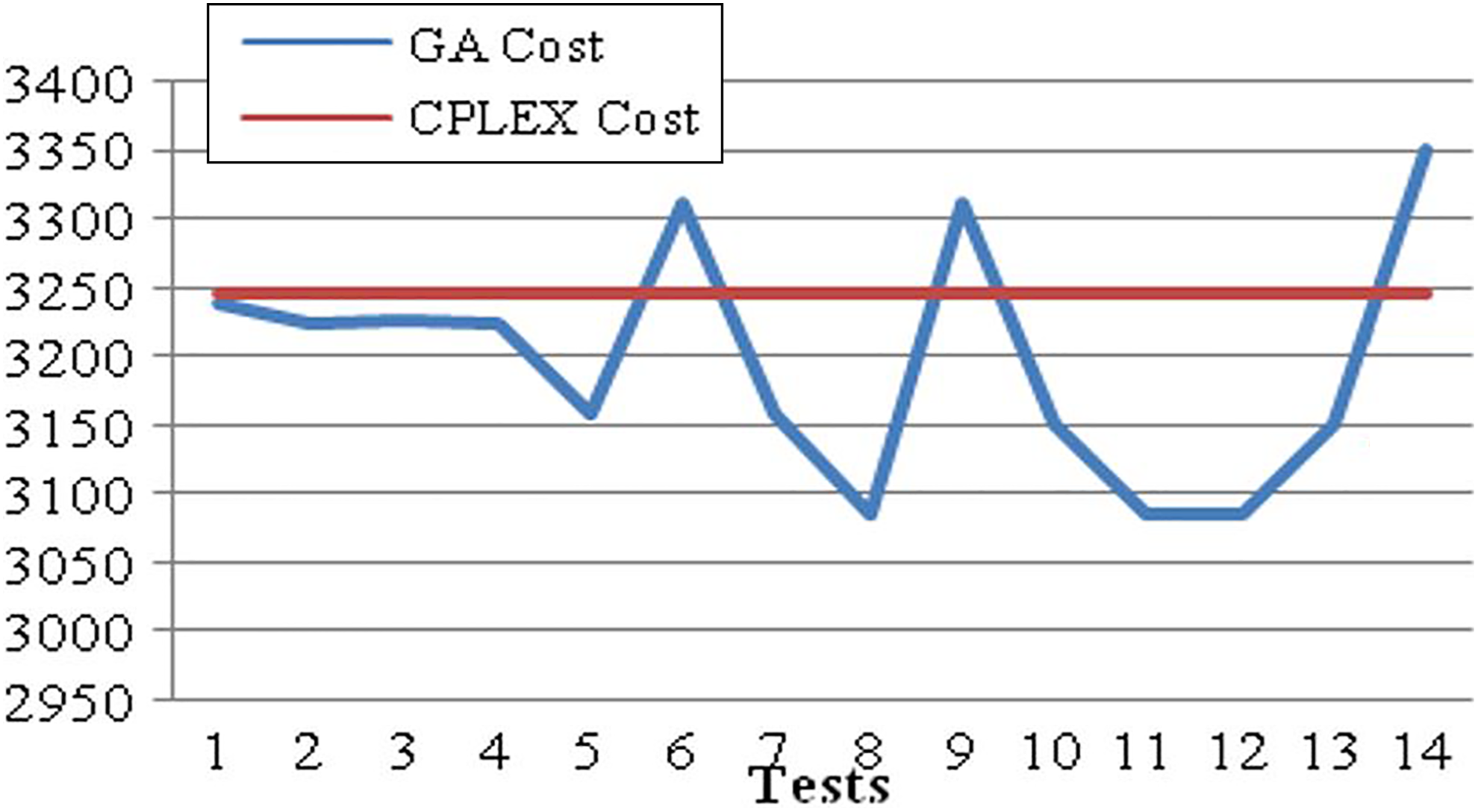
Then we sum the maintenance and the production costs by the various cycles; we obtain the results indicated in Figure 6. We can conclude that the optimal integrated cost for a maintenance cycle is T = 5τ with the total cost equal to 3538.32. The preventive replacements must be done every 5 months and the production planning has to be defined using the GA heuristic with a population size equal to four. We also remark that T = 2τ can be a minimum, since the cost of 3675.48 is near to the previous cost.For a population size equal to four and after a set of experiences of our GA, we found different values of production cost which are neighbor to 3247. As shown in Figure 7 and Table 5, the minimum of the values obtained is CP = 3085 for a max_iteration of 1000. The obtained production planning using GA optimization is different than the CPLEX solver result since the cost is minimized (see Table 6).

Figure 6.

The integrated cost with CPLEX.

Figure 7.

Comparison of results.

Table 5.

Genetic algorithm results.

Iteration number	Production cost	Time (s)	Appearance number
400	3237	28	2
400	3223	30	2
400	3227	32	1
400	3157	27	2
1000	3085	60	3
1000	3151	54	2
1000	3312	56	1
1000	3350	62	1

Table 6.

Production planning.

T = 5τ; CM = 291.32; CP = 3085; CT = 3376
	Product 1				Product 2
Periods t	x 1t	y 1t	s 1t	r 1t	x 2t	y 2t	s 2t	r 2t
1	3	1	1	0	0	1	0	3
2	2	1	2	2	10	1	0	0
3	0	0	1	1	3	1	0	0
4	2	1	1	0	0	0	0	2
5	0	0	0	1	3	1	2	2
6	2	1	0	1	0	0	0	0
7	3	1	1	0	0	0	0	3
8	3	1	2	1	0	0	0	2
9	1	1	2	1	0	0	0	3
10	0	0	1	2	4	1	2	0
11	0	0	0	1	0	0	0	1

The evolution of the obtained numerical results implies the speed of the solution convergence which is approximately 1 min for the case of 1000 iterations. Based on the results of this case study, we can take this model and its implementation in the GA program as an effective and efficient reference easily transferable to solve other kinds of more complex industrial production systems in the framework of integrated planning optimization.The proposed GA program in this contribution has been implemented to optimize the production cost in order to lead to the integrated optimal plan, regardless of the number of products and periods used in the production system. Given the inability of classical exact methods and the linear integer programming to provide an optimal solution in a reasonable time for larger planning problems, we have moved toward the choice of use of an approximate method that is the offered GA.

Conclusion and future work

Owing to the complex constraints and the variables number presented in this case of problem, reaching the optimal results has not been a simple thing for maintenance and production integrated planning. The GA proposed for this model had to optimize the overall cost so that to look for the integrated optimal planning whatever the number of products and periods used in the production system. It is proved in the section of results how the implemented optimization can provide benefits on reducing costs, namely an upward of 200 € (the basic case study made in Belgium by Aghezzaf et Al. ² ) in each maintenance cycle also concerning the average runtime of the suggested program which is about 1 min. The efficiency of the proposed GA will be compared with other evolutionary algorithms like simulated annealing, particle swarm, and ant colony optimization for future researches. In addition, a multilines constrained problem can be considered for further publication.