
Abstract
Our main contribution is to identify the risks implied by the existence of prolonged regulatory lags. We hypothesize that a likely first response is to reduce OPEX, increasing efficiency. If the lag persists for enough time, a vicious circle of inefficiency, disinvestment, and reduced performance can follow. We use a regulatory episode affecting natural gas distributors in Argentina as a natural experiment, controlling with other Latin American countries’ utilities not exposed to the same regulatory stimuli. We evaluate the relative efficiency of fourteen firms for five countries, in seven years, using Stochastic Frontiers Analysis (SFA). Thus, we perform a regulatory impact analysis (RIA) to assess the consequences on the performance of two idiosyncratic regulatory policy instruments applied in the distribution gas industry in Argentina in the 1998–2021 period (the 2002 Public Emergency Law and the 2016 Integral Tariff Review).
Introduction
After the English privatizations in the 1980s, a new paradigm emerged on regulatory grounds: incentive regulation. With the intent to promote efficiency in the British economy, the “incumbent” paradigm in regulatory issues, known as “Cost Plus” or “Rate of Return” regulation, was replaced by a new one, which is customarily identified with the “Price Cap” or “RPI-X” regulation. A series of variants surged after the seminal work of Littlechild (1983). Economic regulation of public utilities comprehends the setting of tariffs, a definition of investment commitments (both in maintenance and expansion of the capital base), quality of service, and social and environmental goals. Incentive regulatory schemes require specific instruments to regulate quality, avoiding undue cost cuts or reductions in productivity (or safety, or reliability). Thus, the regulation seeks to optimize investments to supply current and projected demand, promote the opportunity for cost recovery, and contemplate subsidies to extend coverage or promote consumption in disadvantaged groups.
In the 1990s several Emerging countries replicated Britain’s experience. After the collapse of the Soviet Union, several utilities were privatized in Eastern Europe, Latin America, and Africa. Argentina mimicked the English experience and privatized almost all its utilities, together with a drastic stabilization plan to cut decades of macroeconomic instability. Unlike in England, in Argentina the concerns were not only oriented towards efficiency: there was the urgency to correct fiscal imbalances of the state, an important part explained by public utilities’ losses motivated by low tariffs because of political considerations. Nevertheless, one decade after the country collapsed again in a severe crisis that motivated political changes, and new policies in the opposite direction. Some privatized enterprises were renationalized in the years following that crisis, and others were set to a policy of “starving the beast”: tariffs were frozen, and companies faced dollar-denominated liabilities that must serve with devaluated revenues in pesos. At this point, it seems a very specific experience. Are there any lessons for less unstable countries?
Our main contribution is to identify the risks implied by the existence of prolonged regulatory lags. We extract lessons from this case study. Given a tariff’s freezing at levels that are insufficient to cope with increasing costs, the effect on utilities is the same as in the old-fashioned regulatory lag. In the “Cost-Plus” paradigm, tariff reviews are neither automatic nor periodical. In the “Price-Cap” family of regulatory schemes, inflation is addressed by annual indexation to adjust tariffs, plus periodical cost reviews where performance is evaluated, demand projections are made, investments are planned, quality requirements are set, and subsidies are considered. Thus, considering this case as a (very) prolonged regulatory lag, what is expectable? How will the firms’ efficiency react in the short run? How will the firms’ performance evolve in the long run? We hypothesize that in the short run, since the extension of the regulatory lag is unknown, the firms would adjust efficiency while they are expecting, sooner or later, tariff increases. However, if the tariff freeze is sustained over time, there will be no more room for further efficiency gains, and performance (profitability, investments, and quality of service) can deteriorate. The performance deterioration ends up affecting efficiency.
To cope with the identification of the impact or regulatory lag, we use two methods. We measure efficiency using frontier methods and performance changes by a Regulatory Impact Analysis (RIA). Our findings indicate that there were efficiency gains within the initial stage of the regulatory lag, followed by a prolonged deterioration in performance while the regulatory lag continued. The sector under study is natural gas distribution in Argentina, where efficiency will be checked including a sample of both Argentine and some Latin American comparable providers (not affected by the tariff freeze), while RIA will rest on Argentine information on performance. We have two caveats around the lessons: first, our results do not assess causality; second, the macroeconomics of the case study is quite idiosyncratic. However, the response of the firms, firstly increasing efficiency assuming the phenomena of regulatory lag as transient, and secondly, deteriorating performance when the tariff freeze is prolonged seems sensible.
After this introduction, the second section is devoted to the regulatory evolution of the gas industry in Argentina, and the third section summarizes the literature on efficiency and RIA in the above-mentioned sector. The fourth section contains an efficiency analysis, while the fifth one develops an RIA. The sixth section presents the main conclusions.
Regulatory evolution of the natural gas industry in Argentina
To give context to the analysis, let us start with a brief history of the sector: In 1922, YPF state-owned oil and gas enterprise was founded. Gas downstream (the basins’ exploitation) remains a monopoly in the possession of YPF, and upstream (transportation, distribution, and commercialization) was in the possession of Gas del Estado (GdE), another state-owned enterprise since the 1940s. In the period before privatizations, natural gas tariffs did not reflect opportunity costs. In the 1990s, the country faced a pervasive process of privatization. YPF -privatized in 1992- continued to exploit downstream, however open to competition, and GdE was vertically and horizontally disintegrated. Transportation was split into TGN and TGS (Northern and Southern gas transporters), while distribution and commercialization were divided into eight regional distributors (nine since 1999). Transporters and distributors were private-regulated enterprises, and a new natural gas regulator ENARGAS (National Gas Regulatory Agency) was founded.
The natural gas regulatory mechanism introduced in 1992 was a peculiar price cap. Since 1991 indexation to local currency was banned by law, to combat inflationary inertia after decades of high inflation and two recent hyperinflation processes. Nevertheless, the law admitted indexation to foreign indexes as well as pegged local currency to the US dollar. Thus, the price cap indexation was implemented through the Producer Price Index (industrial goods, basis 1967 = 100) of the US (US PPI for short). There were two correcting factors, -X (to address efficiency gains) and +K (to remunerate extra investments). There were also two seasonal adjustments in the gas (commodity) price. The price cap was intended to last five years, and an Integral Tariff Review was celebrated for the first and last time in 1998 (1998-ITR). In the year 2000, because of a deep recession in the Argentine economy, the US PPI adjustment was suspended, and because the country was immersed in a profound economic, social, and political crisis, in 2002 tariffs were frozen.
As Chisari and Ferro (2005) suggest, “The regulatory framework of privatized utilities in the 1990s in Argentina was constructed under the implicit assumption of macroeconomic stability and sustainability… The privatization process was successful in terms of expanding coverage, increasing productivity and reliability, and fostering investments… But… [a] recession started at the end of 1998, and from 2001 to 2003, the economy underwent a dramatic crisis. A big [currency] devaluation was followed by an 11% fall of GDP and a rise of the rate of unemployment to 24% [in 2002 … After] almost 11 years of a currency board (that pegged the parity between peso and dollar), … [these events were] followed… [by] a generalized default on financial contracts… For sectors under regulation, the contract clauses that established tariffs fixed [and sometimes indexed] in dollars were not respected, and tariffs remained frozen in nominal pesos [when the peso had been devalued a rough 75% in a few months]. Had they been adjusted… customers’ arrears and delinquency would have put a [limit to real tariffs recovering] … Political unrest delayed a long-run solution, and the government initiated a cryptic process of renegotiation [which lasted 14 years]”.
The Public Emergency Law 25561, enacted in 2002 prohibited indexation using foreign price indexes, maintained the ban on indexation in local currency, froze tariffs in nominal pesos, and transformed the dollar-denominated debts of the concessionaires in pesos at the 1.40 pesos per dollar parity in January 2002 (because the initial devaluation was 40%, from 1 peso = 1 dollar to 1.40 pesos = 1 dollar in December 2001, a month during which five presidents were changed, but uncertainty caused that final parity reached 4 pesos per dollar in August). The tariff freeze lasted for almost fifteen years. During this time, costs had increased, and the local currency had continued to devalue. Only marginal adjustments had been made to recover the financial health of the firms. In 2016, an Integral Tariff Review (2016-ITR from now on) was called, tariff adjustments were decided, the capital basis and the cost of capital were estimated, and gradually tariffs started to rise. However, in 2019, after new political changes, tariffs were frozen again, by Law 27541, on equity grounds.
All these events had consequences on the efficiency, and financial health of the concessionaires, investments, and quality of service, some of which we would like to address. Enterprises implemented several policies oriented to avoid further deterioration in their financial condition when tariffs were frozen in 2002: Renegotiation of terms, conditions, rates, and currencies with creditors, claims before the International Centre for Settlement of Investment Disputes (ICSID), and sales of stock packages. Unlike the oil industry, gas companies were not re-nationalized in Argentina.
Literature review on relative efficiency and RIA in the gas industry
Efficiency in the natural gas distribution industry
The simplest possible approach to compare the efficiency of different “Decision-Making Units” (or DMUs, which can be factories, branches of a bank, schools, countries, etc.) consists of computing simple output/input ratios of partial productivity or costs/output ratios of average costs. These are first approximations but do not consider probable complementarities or substitution between inputs, or synergies of joint production in outputs. Most complex techniques use frontier approaches, such as mathematical programming methods and econometric estimates. Of mathematical programming methods, the most used is Data Envelopment Analysis (DEA), and of regression ones, the most popular is nowadays Stochastic Frontier Analysis (SFA). Each one has relative advantages and disadvantages. DEA is flexible and can be performed with small databases and SFA demands decisions on the functional form of the relationship to be estimated and needs more extensive databases. On the other hand, it offers well-documented statistical tests of the validity of the results and usually follows some theoretical guidance on the hypothesis of the relationship between variables. For instance, estimating production or cost frontiers alongside the recommendation of microeconomic foundations (Battese & Coelli, 1988).
By grouping the works surveyed in which the efficiency of service providers is determined, according to the methodology used (parametric or non-parametric), we find: • •
RIA
There is a rich recent academic literature devoted to RIA, after its origin in a seminal document due to OCDE (1997), which defines RIA as a method to evaluate systematic regulatory impact. Harrington and Morgenstern (2004) propose three types of tests to be applied to regulatory measures on an ex-post basis. OCDE (2004) offers a manual for several tests aimed at the regulatory process, efficiency in regulation, and quality of regulatory decision-making. Kurniawan et al. (2018) highlight that the RIA absence can harm the coherence and transparency of regulation. Rogowski and Joński (2018) point to the possibility RIA offers to use indirect methods to check regulation results concerning private sector expectations. Yadav and Tiwari (2022) apply RIA to the whole legal regime of India, while in a more restricted analysis, Nerhagen and Forsstedt (2019) apply RIA to transportation planning in Sweden. Beaulieu-Guay et al. (2019) measure through RIA how Canadian regulators react before the satisfaction or dissatisfaction of the public to regulatory proposals. For Brazil, de Carvalho et al. (2019) propose RIA to evaluate the potential specific effects of a regulatory measure on water and sanitation services. Shah (2018) uses RIA to justify and prioritize different efficient options for street lighting in Antigua and Barbuda.
In Latin American countries the only documented studies of RIA we know were made in Colombia, Brazil, and Chile. In Colombia, Decree 2696/2004 gave a framework to evaluate the regulation’s impact, verifying whether the results adjusted to regulatory objectives. Another exception is Brazil, where the power regulator (Agência Nacional de Energia Eléctrica, ANEEL), developed RIA studies as complementary documentation of main regulations or technical norms. ANEEL uses RIA to check if the potential benefits of the measure overcome estimated costs. In 2021 ANEEL issued a guide for RIA assessment (Ministerio de Economia do Brasil, 2022). More partial is RIA developed by Chile by Law 20199/2017 for natural gas (modifying a previous decree), and by Peru by Law 25844/1992 for the electric industry. The World Bank Group (2021) compiled a database with RIA in different countries.
Efficiency analysis
Data
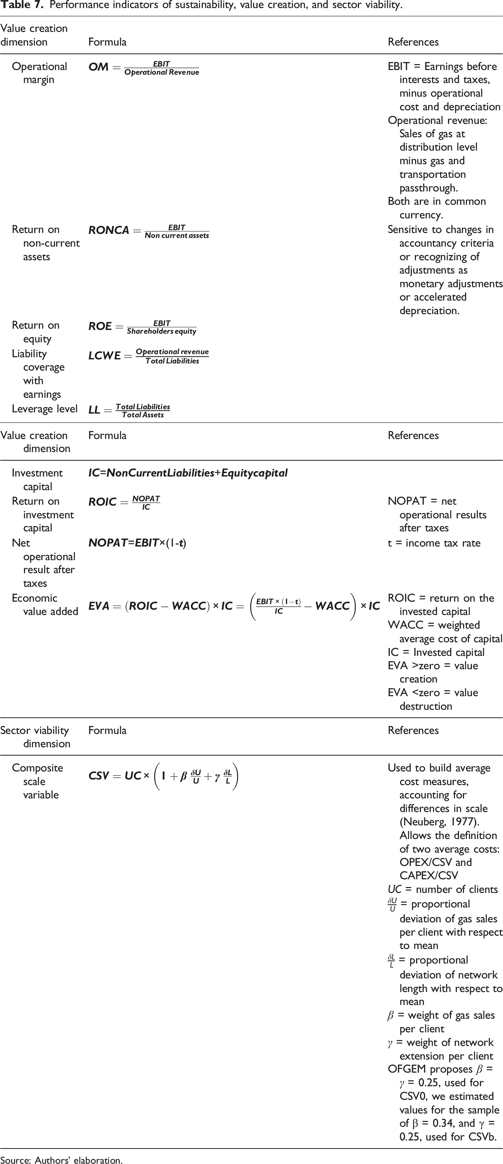
To assess relative efficiency, we built a database, where the units of analysis are utilities, including OPEX, and TOTEX (OPEX + CAPEX), both to be considered as dependent variables in cost efficiency estimates, and the outputs are understood as the cost drivers. The outputs are the number of clients, the volume of gas, and the network length. All these products were combined into a single variable to address the scale of the distribution companies (Composite Scale Variable or CSV), following the methodology applied by the British energy regulator (OFGEM 1999) based on Neuberg (1977). The author argues that network industries are generally characterized by three variables that significantly impact service costs: The number of customers, the Volume of products or services distributed or billed, and Network length. According to Neuberg, the main indicator of scale is given by the number of customers, however, it is common to find companies that, even with a similar number of customers, present significant differences in other variables such as the volume billed or the extension of the network, thus, for the same number of customers, the differences in costs should be explained by the differences in the ratios km of network/customers or energy billed/customers.
OPEX and TOTEX were initially expressed in US dollars, however, we adjusted them according to the IMF Purchasing Power Parity index since relative prices and cost of living are not alike in the different countries of the sample.
To perform an efficiency analysis, we must carry out a study of the companies’ manageable variables. Therefore, any difference in costs must be purged of the effect of “non-manageable” variables. This debugging can be implemented in two ways: (1) including dummy and control variables as explanatory variables in the analysis; and (2) implementing an explicit adjustment in the explained variables (in our case OPEX and TOTEX) for the difference in the non-manageable variables (e.g., salaries, country risk, density, network extension, specific consumption, etc.). In our paper, we use the second option because having a homogeneous unit cost variable is considered a key performance indicator and allows a clear and simple observation of relative efficiency across companies. This is powerful because, specifically and homogeneously, it allows us to determine the cost per equivalent customer.
Consequently, to avoid failures in the control and interpretation of inefficiency, we proceeded as follows: the effect of the physical variables that are not controllable by the management of the companies and that affect the costs of service provision on efficiency was captured by the composite scale variable (CSV). This CSV includes the effect of density and the specific consumption of each company.
As an example, to OPEX efficiency, recalling that such costs are composed of personnel, third-party services, materials, and other accounts, there is a salary difference variable that cannot be managed by the company (which is rather explained by productivity differences or idiosyncratic issues) that explains more than half of them. The rest of the operating costs (materials and others) are partly explained by physical conditions (the firm’s maintenance costs are associated with network km and this is captured by the CSV). Therefore, having largely adjusted for cost differences not attributable to management, the remainder that would exist in OPEX is a good measure of the inefficiency observed in OPEX.
Regarding the CAPEX variable, the impact of country-specific conditions on the capital base is captured by CSV in the TOTEX analysis. Regarding the cost of capital rate, it was calculated homogeneously for each country considering the country risk calculated by JPMorgan. As in the case of OPEX, the difference observed in TOTEX would reflect the inefficiency of the companies.
Once costs are homogenized, adding dummies would capture the remainder of the cost difference and would probably place all companies close to the efficiency frontier. We performed also different alternative versions of the models, including those in which instead of considering a synthetic measure of production as CSV, we decompose it into its main components (clients, gas, and density), and we also added dummies to address country differences (and we could also add dummies to address company differences). The problem is that when you add all these variables the average efficiency converges to units and there are no sensible differences between companies and years in their efficiency performance. We also employed two versions of CSV: The one with the weights assigned in the original paper of Neuberg (1977) and the one with the weights we computed for our sample of Latin-American companies (CSVb), which are slightly different. Thus, we choose to maintain a parsimonious model containing only CSV (with the weights for LATAM companies.
A detailed explanation of the adjustments in wages is presented in the Appendix.
Efficiency assessment, variable definitions.
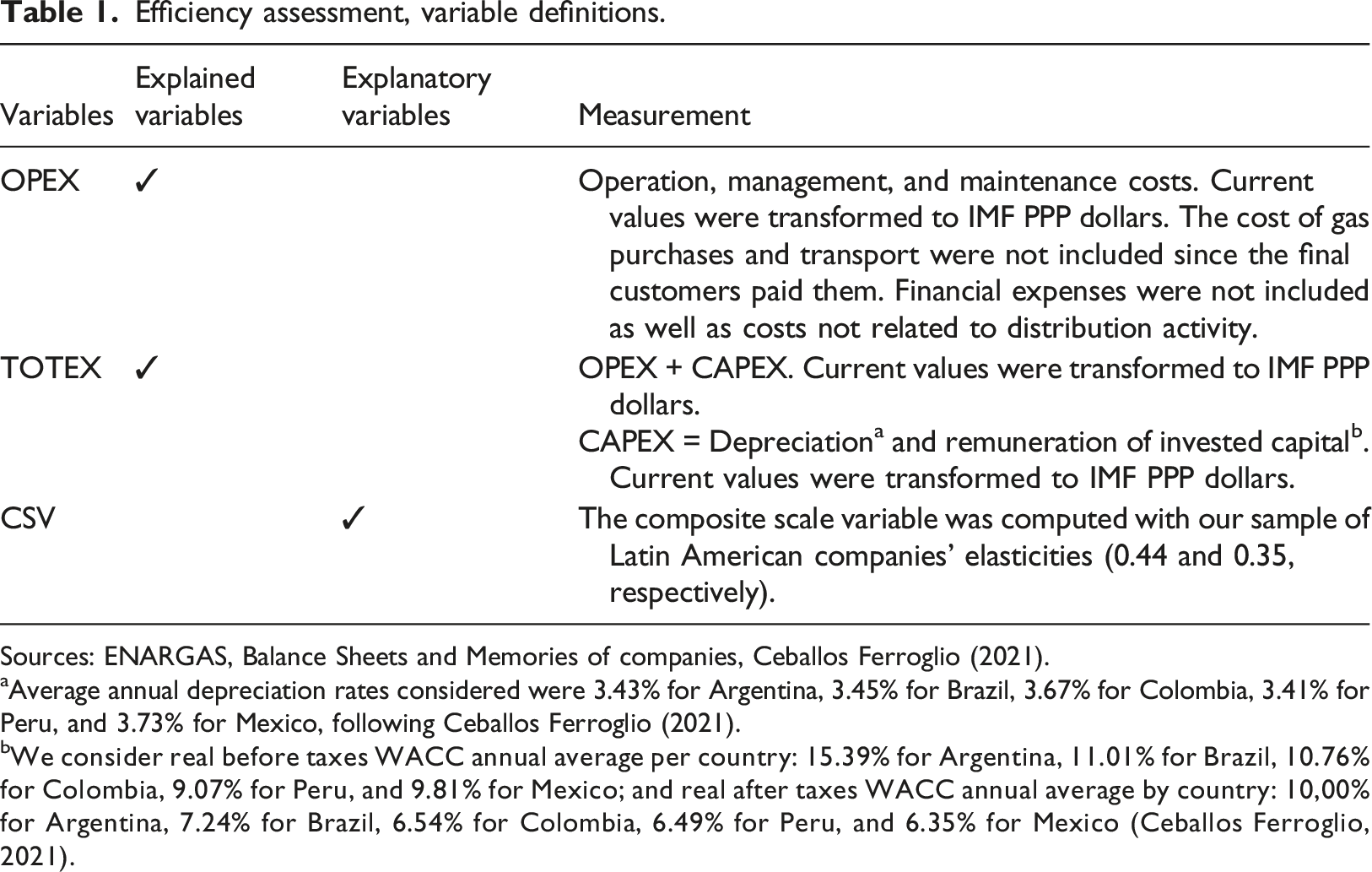
Sources: ENARGAS, Balance Sheets and Memories of companies, Ceballos Ferroglio (2021).
aAverage annual depreciation rates considered were 3.43% for Argentina, 3.45% for Brazil, 3.67% for Colombia, 3.41% for Peru, and 3.73% for Mexico, following Ceballos Ferroglio (2021).
bWe consider real before taxes WACC annual average per country: 15.39% for Argentina, 11.01% for Brazil, 10.76% for Colombia, 9.07% for Peru, and 9.81% for Mexico; and real after taxes WACC annual average by country: 10,00% for Argentina, 7.24% for Brazil, 6.54% for Colombia, 6.49% for Peru, and 6.35% for Mexico (Ceballos Ferroglio, 2021).
Descriptive statistics a .
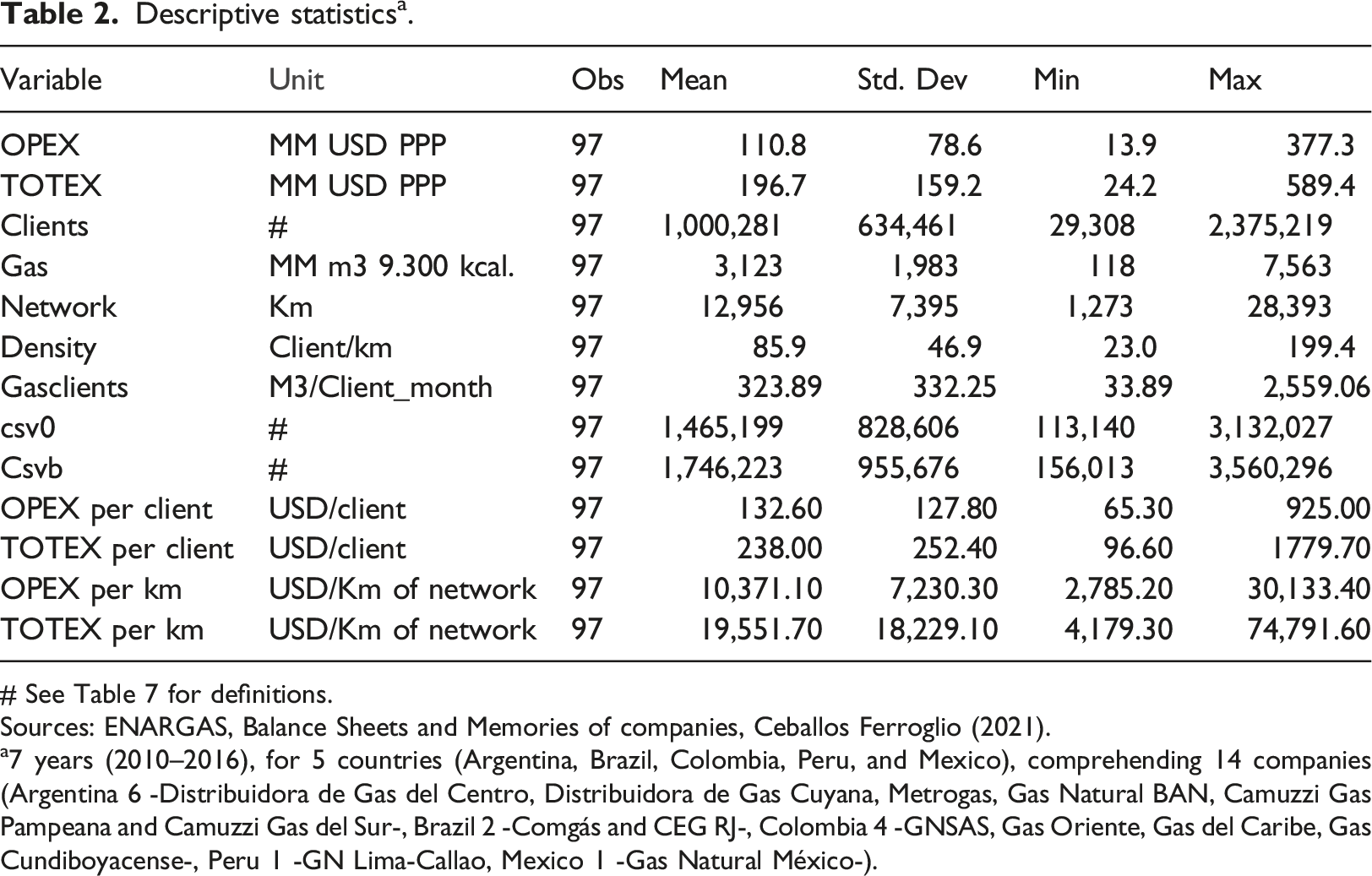
# See Table 7 for definitions.
Sources: ENARGAS, Balance Sheets and Memories of companies, Ceballos Ferroglio (2021).
a7 years (2010–2016), for 5 countries (Argentina, Brazil, Colombia, Peru, and Mexico), comprehending 14 companies (Argentina 6 -Distribuidora de Gas del Centro, Distribuidora de Gas Cuyana, Metrogas, Gas Natural BAN, Camuzzi Gas Pampeana and Camuzzi Gas del Sur-, Brazil 2 -Comgás and CEG RJ-, Colombia 4 -GNSAS, Gas Oriente, Gas del Caribe, Gas Cundiboyacense-, Peru 1 -GN Lima-Callao, Mexico 1 -Gas Natural México-).
The final specification of the parametric frontier models considers that the main objective of the analysis is to determine the management efficiency of the distribution companies, considering two main dimensions of service provision: A technical or physical one and an economic one. In terms of the technical dimension, the CSV allows for capturing the main differences in the technical conditions of service provision, such as the density of consumers per network kilometer and the average gas consumption per client.
As for the economic dimension, both OPEX and TOTEX are homogeneous variables across the analyzed countries. The OPEX variable was adjusted to consider the wage differential between countries. The TOTEX variable is homogeneous since CAPEX was calculated by using a WACC (Weighted Average Cost of Capital) and a depreciation rate, both determined for each country from the same database and time horizon and with a single methodology.
Together with the variables we use in the regressions, we compute several average cost measures. The average company spent a mean of 111 million dollars in OPEX and 197 million dollars in TOTEX. The average company of the sample has one million clients. Thirteen thousand kilometers of network and 3.123 million cubic meters of distributed gas, annually; nevertheless, the smallest company has only 29 thousand clients. The average density is 86 clients per network kilometer. The sample is made of 97 observations, and it is almost a balanced panel (we do not have data of one Colombian company for 2016), of 7 years, and 14 companies (from 5 different countries). 1
Method and models
We use the SFA standard model for estimating efficiency in cross-sectional databases, even when we can implement the problem as a panel data estimate (Kumbhakar & Horncastle, 2015). It can be written as:

The expression (2) indicates that the observed production (cost) is below (above) the efficient output (cost), being the efficient unit i output (cost): lnyi*=ln[Y(x i ;β)+[Y i (x i ;β)+υ i ].
The term u
i
is the log difference between the maximum (if it is a production frontier), or minimum (if it is a cost frontier) lnyi* and the actual output (cost) lny
i
or the percentage by which actual output (cost) can be increased (reduced) using the same inputs (producing the same output) if the unit is fully efficient. The estimated value of u
i
is referred to technical (cost) inefficiency, with a value close to zero implying closeness to full efficiency.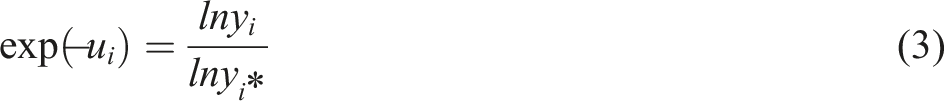
Parameters of the SFA and the model for the technical inefficiency effects are estimated simultaneously by maximum likelihood. The parameter
The real functional form is unknown, being the more common choices the Cobb-Douglas, and the Trans logarithmic (or “Trans log”), which addresses squared and interaction terms of the variables. We use two Cobb-Douglas cost specifications in logarithms: an OPEX and a TOTEX, where each cost component depends on the logarithms of CSV. The variable CSV considers the elasticities calculated from the sample of Latin American companies.
We use CSV for several reasons: the information the variable condenses, and the possibility of working with a relatively small database estimating only two parameters (a scale elasticity and a constant). We run alternative models including separately the variables that compose CSV and controls for each country to address the heterogeneity of countries (see Table A2, in the Appendix).
Estimates
SFA normal/half normal models (lOPEX and lTOTEX as dependent variables).
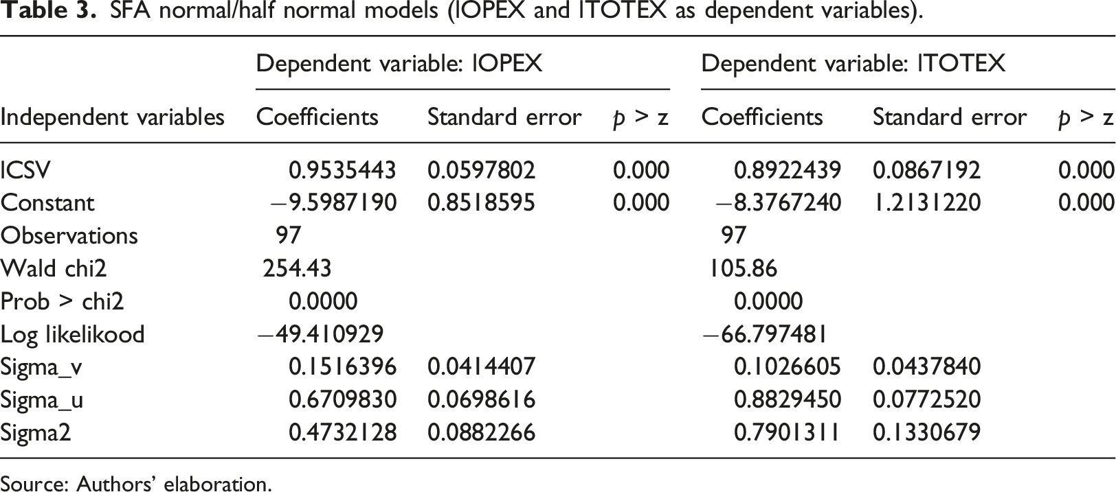
Source: Authors’ elaboration.
Discussion of the efficiency results
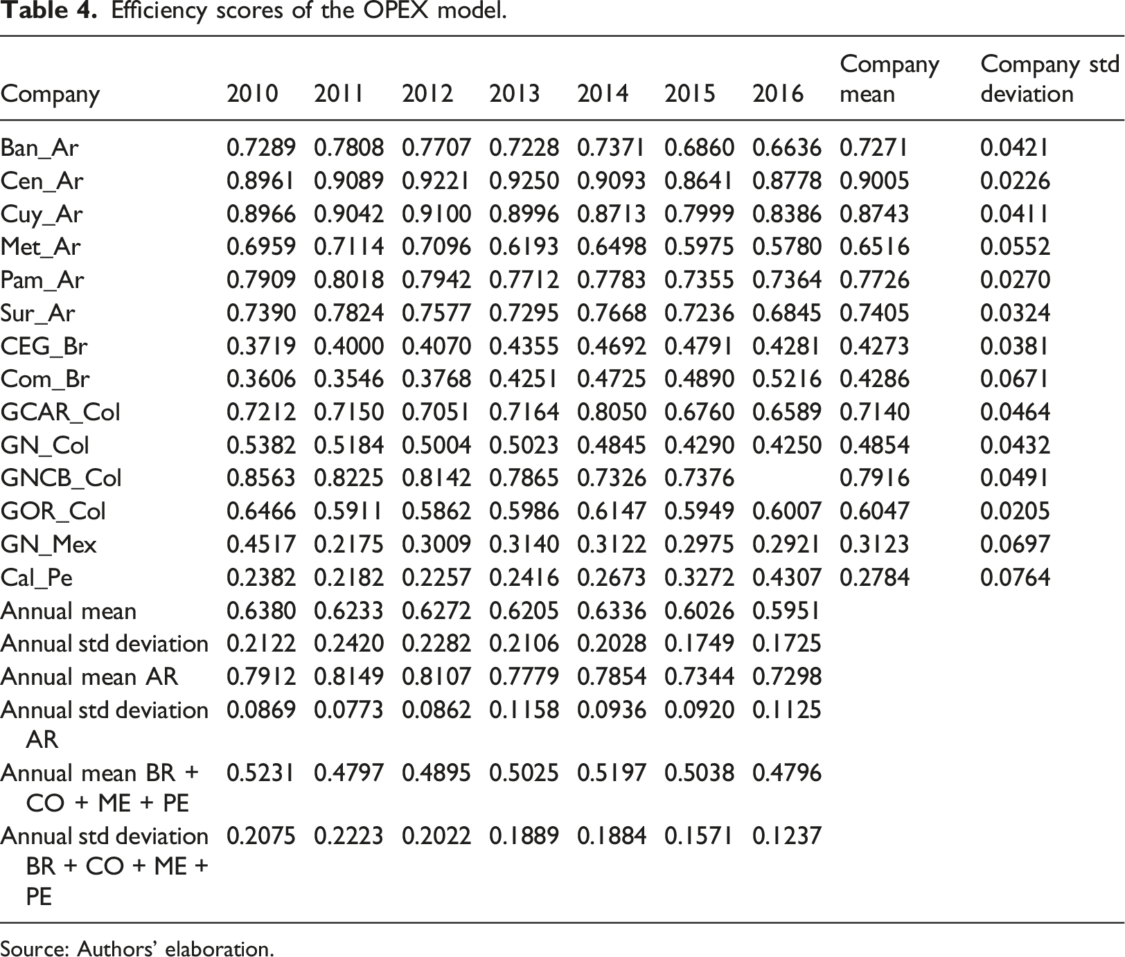
Efficiency scores of the OPEX model.
Source: Authors’ elaboration.
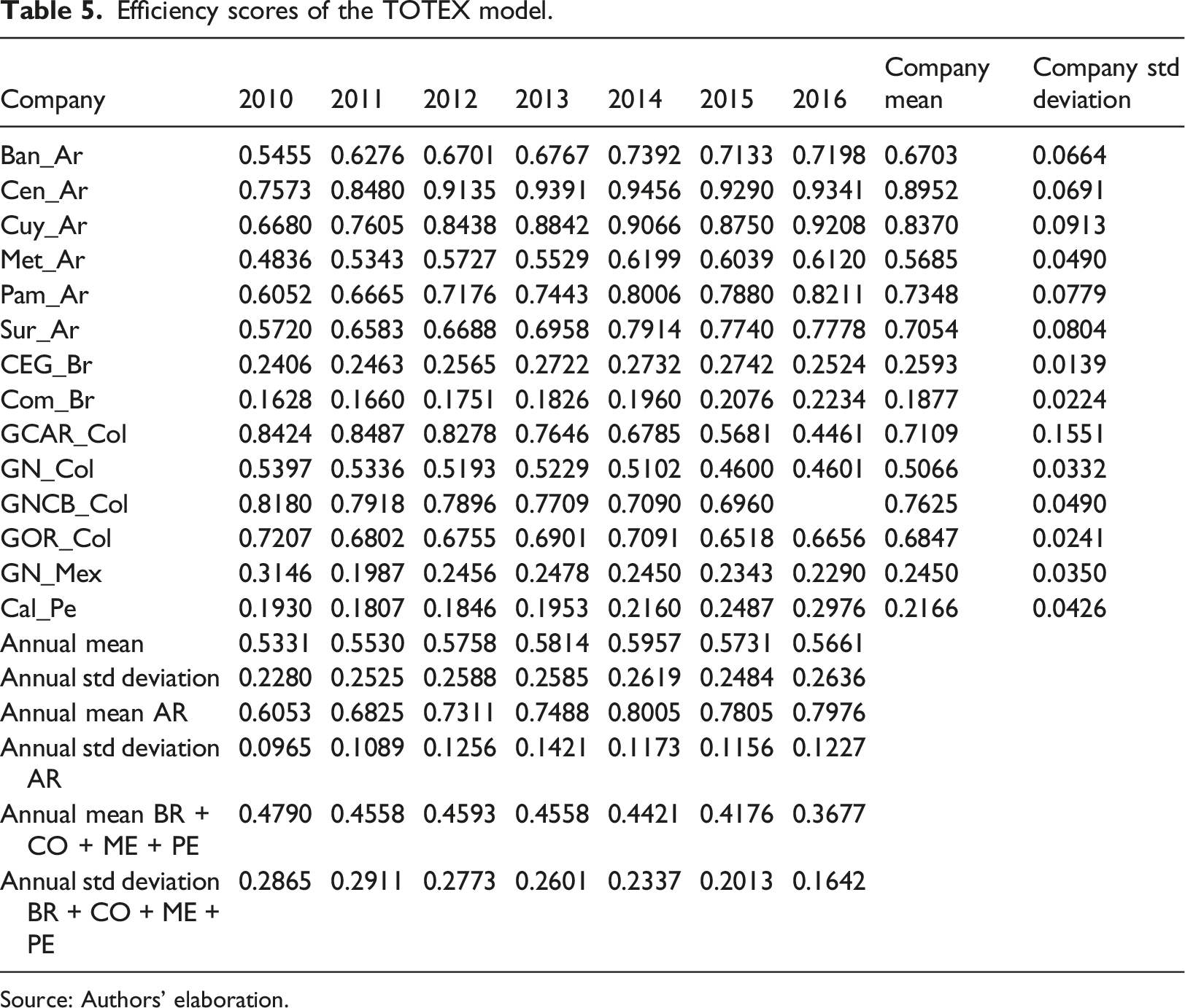
Efficiency scores of the TOTEX model.
Source: Authors’ elaboration.
Regarding the OPEX variable, and analyzing it in terms of efficiency level, the average efficiency of the Argentine companies is significantly higher than the rest of the companies in the sample (compare rows “Annual Mean AR” and “Annual Mean BR + CO + ME + PE in Table 4). This is due to the long regulatory lag that forced companies to become extremely efficient to survive. Regarding this, it should be clarified that there are no significant differences between the fundamentals of different countries as the information was standardized. An example of this is the adjustment made for the variable of salaries, where information from the Union Bank of Switzerland was used. Similarly, the cost of capital rate for different countries was estimated for the same years, using a uniform methodology (CAPM-WACC). The other variables were standardized using a parity exchange rate to homogenize them. Thus, it can be concluded that the differences primarily stem from the policy instrument utilized.
For the case of TOTEX, the same considerations as for OPEX were made, meaning the efficiency scores for the total costs function are displayed.
Regarding TOTEX, the efficiency level analysis shows that, on average, Argentine firms are significantly more efficient than the average of the others, and additionally, this efficiency difference increases to double the average efficiency of the region’s firms (compare rows “Annual Mean AR” and “Annual Mean BR + CO + ME + PE in Table 5).
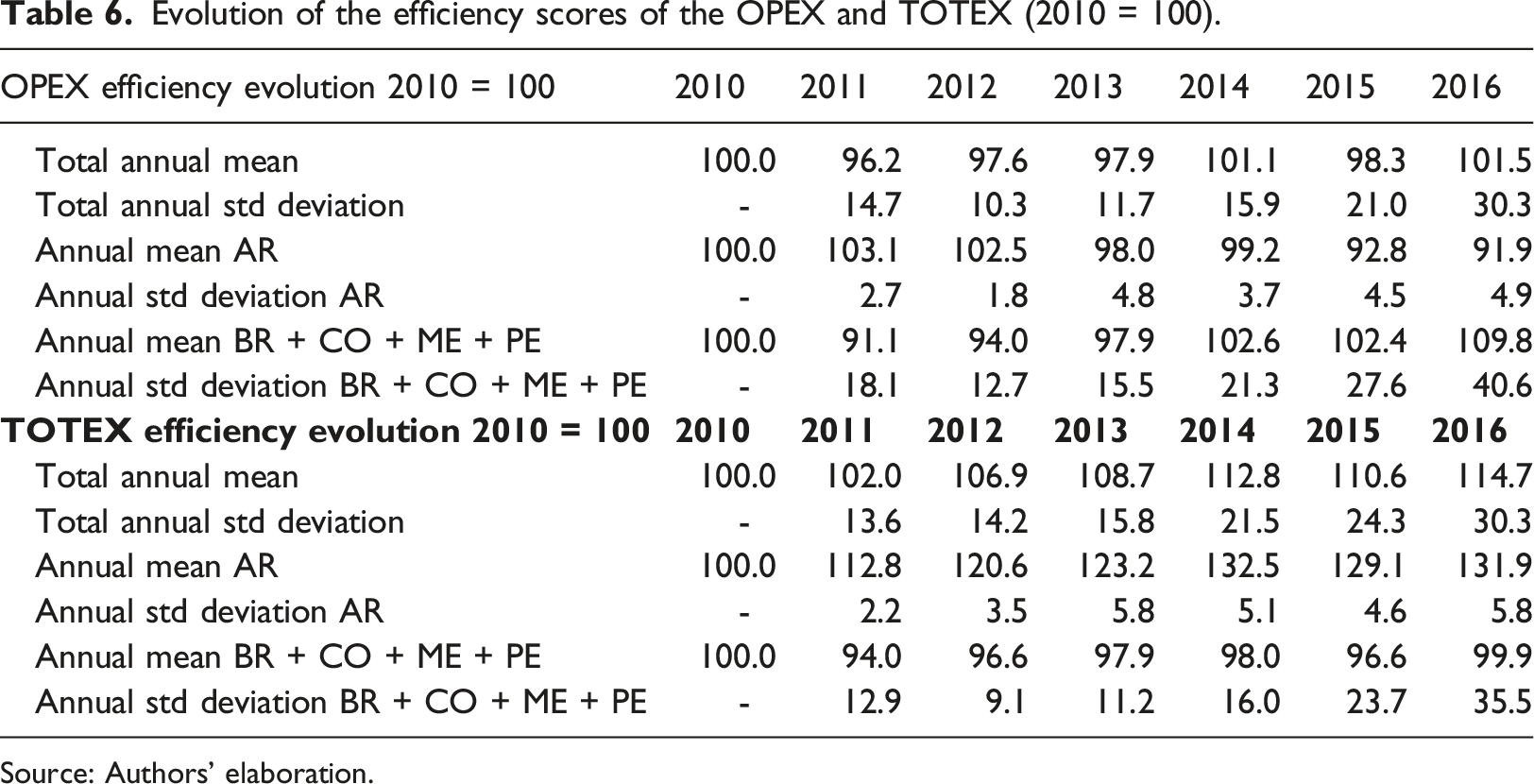
Evolution of the efficiency scores of the OPEX and TOTEX (2010 = 100).
Source: Authors’ elaboration.
RIA assessment for the natural gas distribution industry in Argentina
We analyze the companies’ performance before two important regulatory episodes: (1) The sanction of the Law of Public Emergency 25561/2002 which denominated tariffs in nominal pesos and froze them after a currency devaluation and eliminated tariff indexation according to US PPI. (2) The 2016-ITR removed the freezing and started to recover tariffs in real terms. We identify episode (1) as the start of the regulatory lag, and episode (2) as the end of the regulatory lag. Inflation, which was not a problem in 2001, increased in the country after 2002, and accelerated in 2007, thus tariffs became eroded in real terms during the regulatory lag period (2003–2016).
3
Our RIA consists in applying a means difference test on a set of financial and commercial indicators, associated with several dimensions of the service. We specify a null hypothesis H0, a significance level α, and we compute a p-value. If this p-value is lower than α (t > t-critic), H0 is rejected, and the conclusion is that the differences are not random and that the population means are different.
If population variances are unknown and assumed different, the test for the H0: μX - μY = δ is based on the statistic of Welch (1947) test: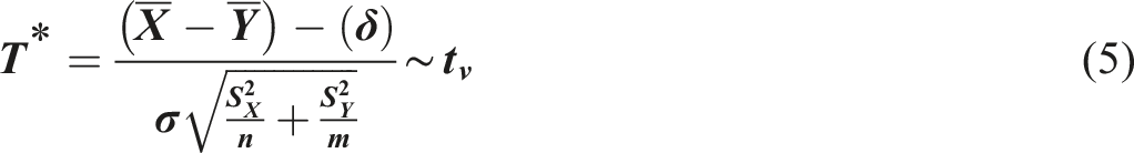
T* is distributed as a t-Student, with approximately ν degrees of freedom when H0: μX - μY = δ is true, being ν < n + m−2 and estimated according to: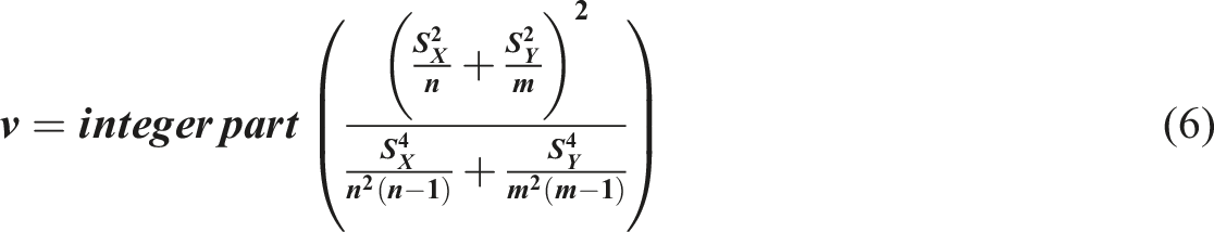
Structural modeling with Kalman filtering was applied to each of the series analyzed using Stamp v8.3 software and based on the econometric methodology of Harvey (1981 and 1989), according to which, the behavior of a series can be explained by a trend, a slope, a seasonal factor, and an irregular (random) shock. All components follow stochastic processes, but special deterministic cases may occur, or some components may be absent (Franzini & Harvey, 1983). Structural modeling helps to identify what type of effect a policy instrument generates on a series.
Indicators
Performance indicators of sustainability, value creation, and sector viability.
Source: Authors’ elaboration.
Data
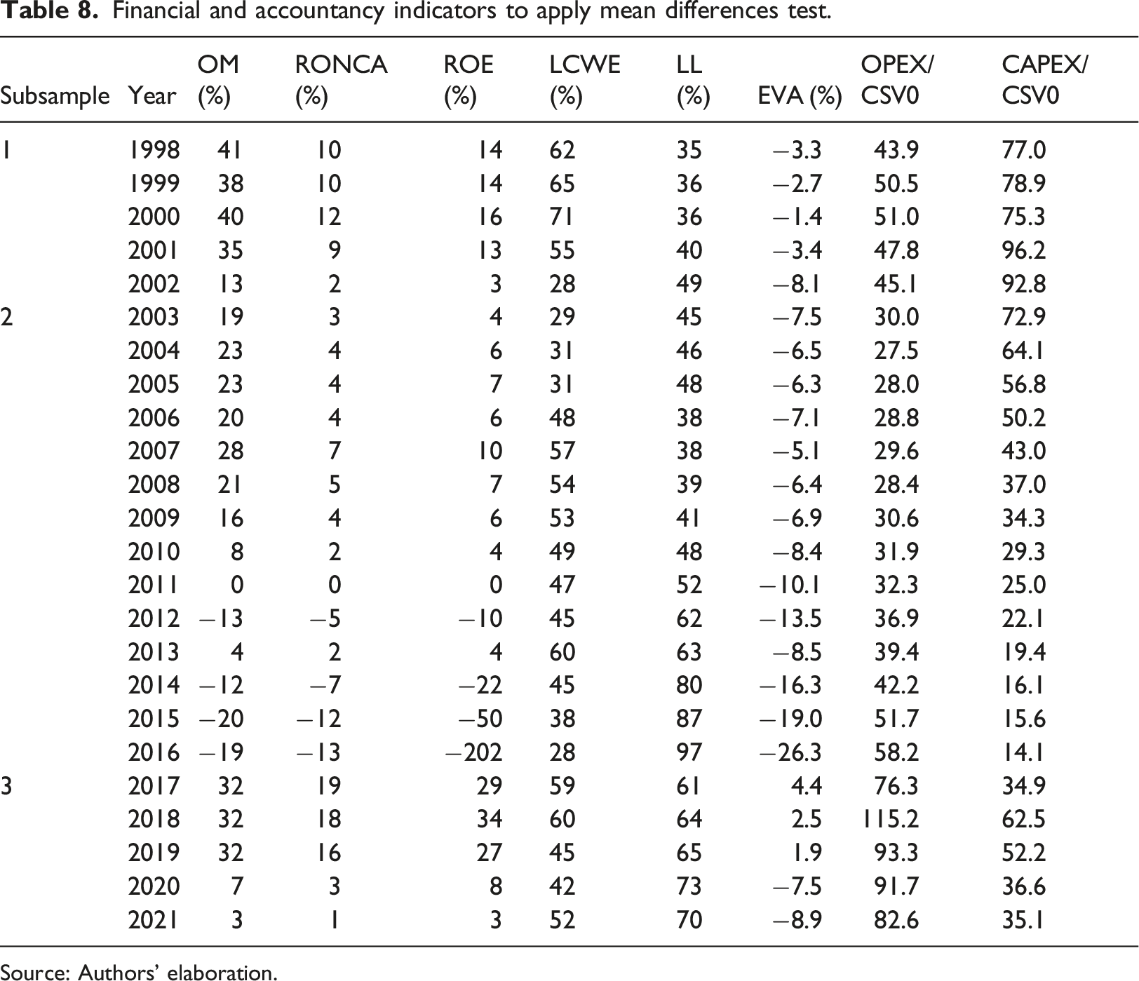
To calculate the performance indicators used in the RIA, we use a database with accounting information for the period 1998–2021 for five gas distribution companies in Argentina (Cuyana, Metrogas, BAN, del Sur, and Pampeana). 4
The accounting information used in the analysis of the sectoral sustainability dimension is based on the balance sheets and income statements of the distribution companies. The accounting basis has annual information for the entire period analyzed.
The commercial indicators are derived from a database with information on the number of customers and volume of gas distributed published by ENARGAS. Key performance indicators referring to operating costs per equivalent users and capital costs per equivalent users were also calculated.
The capital cost rate approved in the 2016-ITR was calculated at 9.33% after taxes and applied in the calculation of the tariffs in force as of 2017. Therefore, to determine the remuneration of capital for the whole period, a rate of 10% is assumed. 5 Both operating costs and capital costs are expressed in 2021 dollars.
Results
Financial and accountancy indicators to apply mean differences test.
Source: Authors’ elaboration.
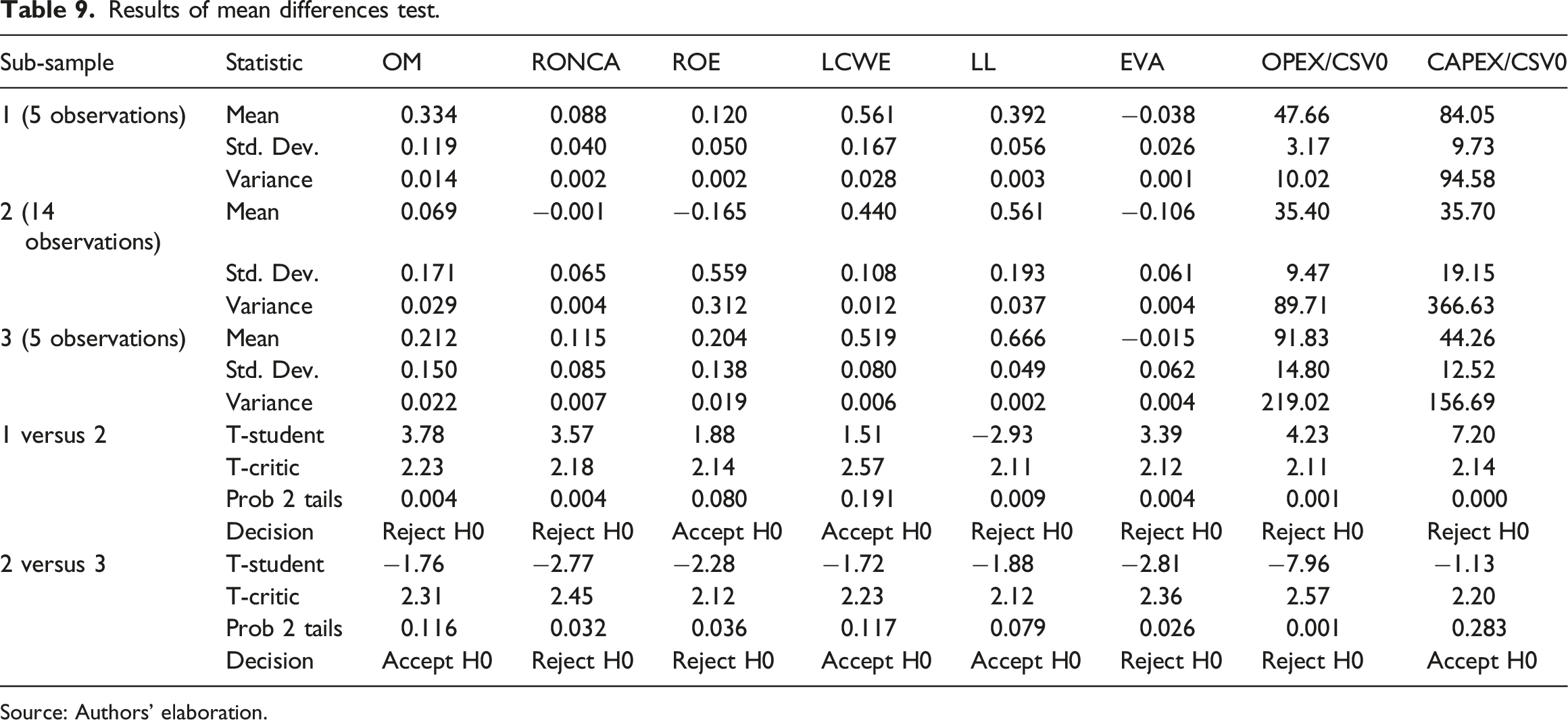
Results of mean differences test.
Source: Authors’ elaboration.
In the comparison of subsamples 1 versus 2, the null hypothesis that the means of the subsamples are equal in the case of the ROE and LCWE could not be rejected. This implies that the Public Emergency Law could not mark a significant change in the two indicators. For the remaining ratios, the null hypothesis is rejected, which implies that the regulatory instrument generated a significant change in them between both periods. In addition, the effect of the regulatory instrument translates into a deterioration in profitability and a general deterioration in all dimensions of service provision.
Regarding the comparison of subsamples 2 versus 3, the null hypothesis of equality of means is accepted for the indicators OM, LCWE, LL, and CAPEX/CSV. Thus, even though the 2016-ITR was not enough to generate a statistically significant change in the operating margin, and in the indebtedness indicators. On the other hand, there was a statistically significant change in the ROA and ROE indicators, partly because together with the implementation of 2016-ITR, there was a methodological change in the accounting rules, since IFRS standards were adopted, and because of the 2016-ITR process, there were adjustments, revaluations, and reductions in the asset base as well.
Another indicator showing significant changes is the OPEX/CSV, explained by the inflationary process observed in the last years of the period under analysis. Cost per client, under inflationary processes, is mainly determined by factors exogenous to the company’s management. The 2016-ITR did not restore the Price-Cap mechanism before 2002 and the sector is in practice regulated as a Cost-Plus.
A state-space analysis (Kalman Filter) was also conducted on the series of all indicators to evaluate their behavior and identify whether regulatory lag and RTI policy instruments significantly affected the series. The state space model was applied to all indicators from 1998 to 2021 with a general specification including random level and slope and automatic interventions in determining level breaks and outliers in series. Particular specifications were adopted only in exceptional cases based on the behavior of the indicator. The results obtained are described below:
The OM series is explained by a random behavior in terms of level and slope, registering two “level breaks” in the years 2002 and 2017. This fact statistically ratifies and reinforces the results obtained with the mean difference tests. Public Emergency Law generated a significant deterioration in the OM in 2002, while the 2016-ITR, although it caused a break in level, was not enough to support a significant difference in means.
In the case of RONCA, the general model specification identified a significant and positive breakpoint in 2017. To maintain consistency criteria, manual intervention was added in 2002, resulting in a significant negative breakpoint.
The analysis of the random slope and level specifications of ROE resulted in two-level breaks: one significant, positive break in 2017 (consistent with other indicators), attributed to the effect of ITR, and another significant, negative break in 2016. The latter revealed the accounting and financial issues faced by the distributing companies Metro and Sur, which had negative net worth.
In the case of the LCWE, a random level specification (which was statistically significant but only at a 10% level) and a fixed slope specification were implemented. The automatic interventions produced three significant breaks (in 2002, 2006, and 2017) and one significant outlier in 2013.
Considering LL, the model specification produced a sole, significant break in 2017, albeit with a negative sign due to distribution companies’ indebtedness reduction.
In the EVA analysis, both the level and slope specifications were randomized. Automatic interventions, which caused a level break in 2017, as well as a manual intervention for the break observed in 2002 (with a negative sign), were found to be significant.
In the case of OPEX/CSV0, there were random level and slope specifications, resulting in significant level breaks - negative in 2003 and positive in 2017 - due to manual interventions. As for CAPEX/CSV0, level specifications were also random, but slope specifications were fixed, producing three significant positive breaks in 2001, 2017, and 2018 through automatic interventions. The pauses indicate positive developments resulting from companies’ strategic actions to raise their compensation bases ahead of the tariff revision (2001) and from restored confidence following the ITR process.
The means difference analysis and the Kalman Filter also show that both regulatory instruments had a significant impact in terms of the value creation dimension. The Public Emergency Law caused a decrease in value creation and the 2016-ITR generated an apparent re-compositing in this indicator, though insufficient to create value again.
Gas consumption per client, although relatively stable throughout the 1994–2011 period, had an abrupt drop in 2002 because of the economic crisis of December 2001. From 2012 onwards, there was a downward trend, and in 2021 the consumption was even lower than in the year of the crisis (2002). 6 The connections granted to new customers decreased throughout the period, especially in 2002. Although there was a recovery in the growth rate between 2002 and 2008, thereafter there is a continuously decreasing trend until reaching values like those of the 2002 crisis in 2021.
After the implementation of the 2016-ITR, OPEX grew for one more year but then began a slightly decreasing trend. Similar behavior was observed in CAPEX. There was a first stage after 2016-ITR of higher investment (which led to a reduction in OPEX) but then the decrease in CAPEX was used to maintain profitability margins.
With real income deteriorating, the investment variable became the adjustment path to try to maintain profitability margins. Considering the average in the gas industry during the period analyzed, CAPEX went from representing 71% of the total cost in 2003 to a level of less than 20% percent in 2016. This situation was also reflected in connection expansions, which continued to fall steadily
Conclusions
This paper identifies the risks implied by the existence of prolonged regulatory lags. We analyze the efficiency and performance of selected gas distribution companies in Latin America, focusing on the regulatory lag observed in the Argentine regulatory scheme. We postulate that given a regulatory lag that affects the finances of gas distribution companies, a likely first response is to increase efficiency by reducing OPEX. If the lag persists, the management capacity of the companies sharply deteriorates, culminating in a vicious circle of disinvestment, and reduced performance, where long-run efficiency would be jeopardized.
We first evaluate the relative efficiency of firms in the analyzed countries, using Stochastic Frontiers Analysis (SFA). Two models were specified, one for OPEX and the other one for TOTEX, considering, in both cases, the composite scale variable (CSV) as the explanatory factor. In the case of TOTEX, the observed efficiency was higher for the Argentinean companies, and unlike what happened with OPEX, the increasing trend was observed throughout the whole period. This reveals an adjustment in investments after all possibilities of reducing operating costs were exhausted. The efficiency gains came at a very high cost, in terms of disinvestment and bad financial results for the companies. Regarding the OPEX variable, the average efficiency of the Argentine companies is significantly higher (0.73, and a standard deviation of 0.12) than the rest of the companies in the sample (0.44 and a standard deviation of 0.24). For the case of TOTEX, the same considerations as for OPEX were made.
Our second empirical step is to implement a regulatory impact analysis (RIA) to assess the consequences of two regulatory policy instruments applied in the gas industry in Argentina for the period 1998–2021. The aim was to identify whether the 2002 Public Emergency Law and the 2016 Integral Tariff Review, generated significant changes in the sector performance. The approach consisted of a mean difference analysis on a series of variables representative of different dimensions of service provision and a Kalman Filter. The results of the RIA showed that until 2011 distribution companies, on average, obtained positive profitability, because of the (forced) need to reduce OPEX to maintain profitability margins arising from the application of the 2002 Public Emergency Law. Operational margin was 0.33 on average before the emergency, 0.07 during the emergency and recovered to 0.21 after the emergency. In addition, a reduction in investments was also necessary (CAPEX/CSV drops from an 84 average before the emergency, to 35 during the emergency and recovered to 44 after the emergency). A reduction in the number of new customers and consumption per customer was also observed during the period of analysis. Regarding the variables OPEX/customer and CAPEX/customer, the conclusions obtained in the efficiency analysis were ratified using the RIA analysis. The 2016-ITR generated incentives to increase investments and reduce operating costs, but it was not enough.
Our main contribution is to identify the risks implied by the existence of prolonged regulatory lags; however, it is not a causal analysis. Though based on the case of Argentina, with very peculiar macroeconomics in our period of analysis, some general conclusions could be useful to other developing countries: a delay in the recovery of tariff in real terms, generates negative impacts that are extremely difficult to reverse both, for the companies providing the service and for the current and future users because of the deterioration of the service and the infrastructure conditions. This is expected because of the possible gains of efficiency in the initial stage of the regulatory lag.
Footnotes
Declaration of conflicting interests
The author(s) declared no potential conflicts of interest with respect to the research, authorship, and/or publication of this article.
Funding
The author(s) received no financial support for the research, authorship, and/or publication of this article.
Notes
Appendix
Appendix: Wage Differentials Adjustment and Alternative Models
There is a structural difference in wage costs among countries in the region, which originates from differences in the cost of living, besides exchange rate differences.
Based on the Union of Swiss Banks’ publication of price and wage comparisons for 71 cities around the world (UBS, 2015), the wage costs of three job categories related to gas distribution services were calculated for the countries considered in the analysis: manager (share 20%), engineer (share 60%) and call center (share 20%).
To eliminate wage differences due to purchasing power parity distortions, average wages were adjusted for the differences in the exchange rate used in the UBS study and the parity exchange rate published by the International Monetary Fund. With the aggregate wage cost, expressed in IMF parity dollars, we proceeded to calculate the adjustment coefficient for wage differences, taking Argentine wages as a reference. Since wage costs in Argentina are lower than those in Brazil, for example, to homogenize costs it is necessary to multiply the Brazilian costs by 0.41. The adjustment should be applied only to the fraction of operating costs corresponding to wage costs (approximately 50% of total OPEX).
UBS Salary Index in the services sector in 2015 US dollars. Source: Ceballos Ferroglio (2021).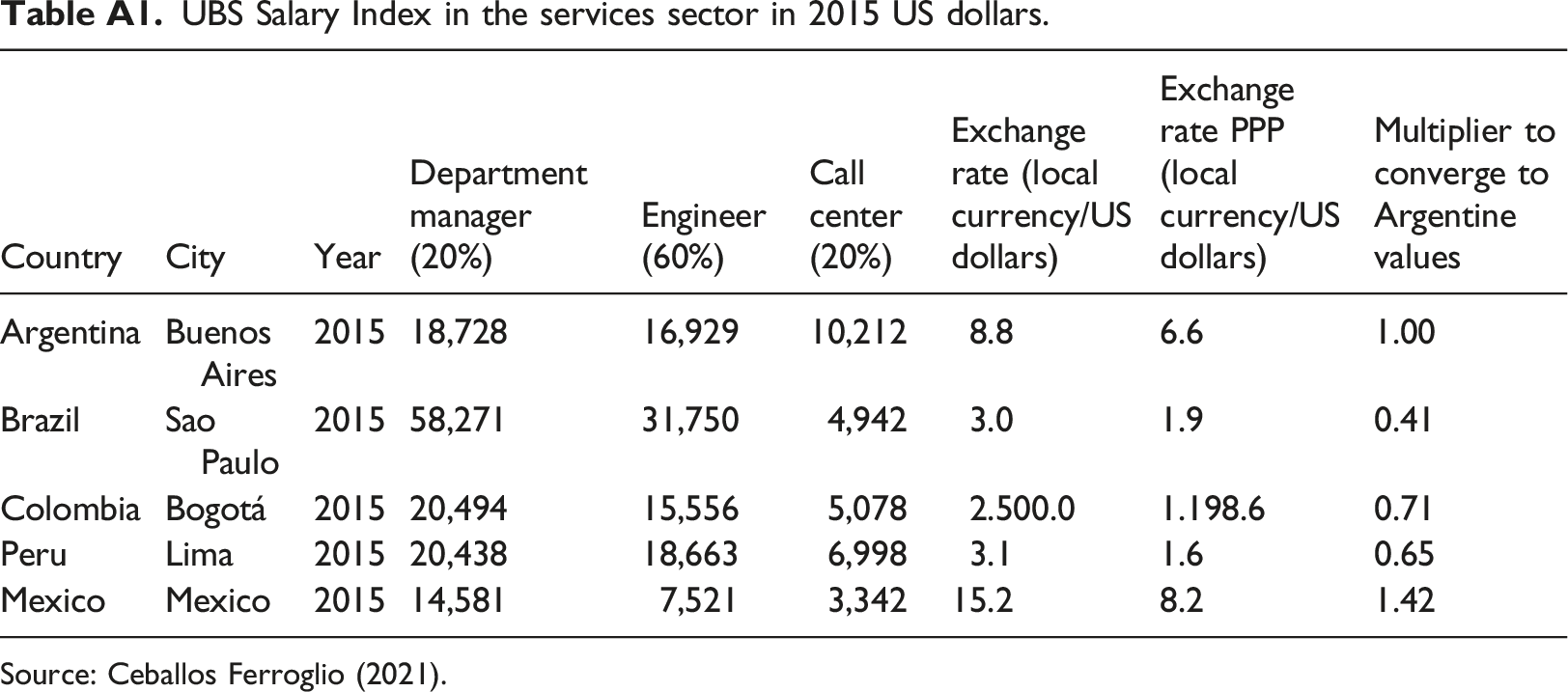
Country
City
Year
Department manager (20%)
Engineer (60%)
Call center (20%)
Exchange rate (local currency/US dollars)
Exchange rate PPP (local currency/US dollars)
Multiplier to converge to Argentine values
Argentina
Buenos Aires
2015
18,728
16,929
10,212
8.8
6.6
1.00
Brazil
Sao Paulo
2015
58,271
31,750
4,942
3.0
1.9
0.41
Colombia
Bogotá
2015
20,494
15,556
5,078
2.500.0
1.198.6
0.71
Peru
Lima
2015
20,438
18,663
6,998
3.1
1.6
0.65
Mexico
Mexico
2015
14,581
7,521
3,342
15.2
8.2
1.42
SFA normal/half-normal models (lopex and ltotex as dependent variables), independent variables alternative to CSV. Source: Authors’ elaboration.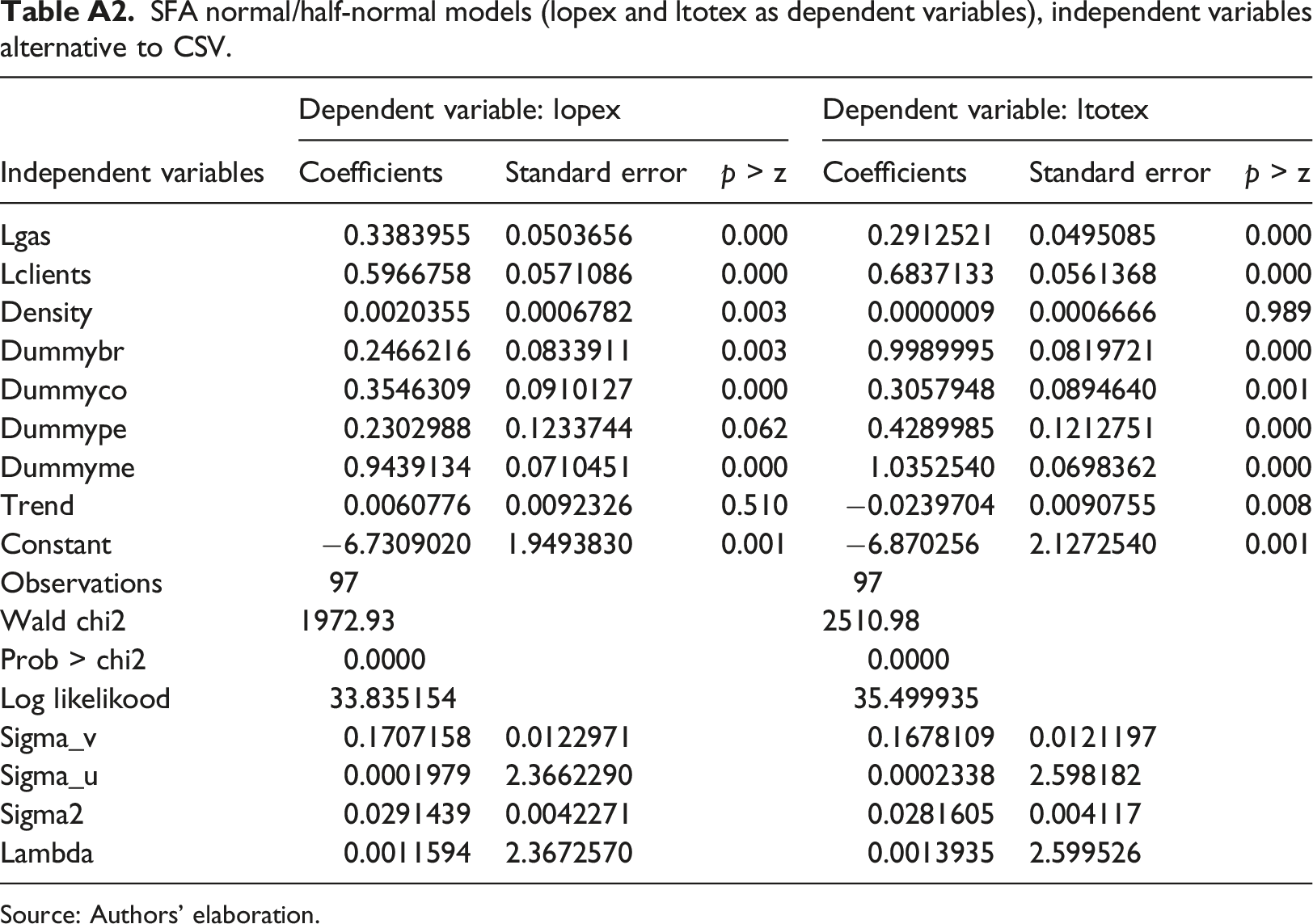
Dependent variable: lopex
Dependent variable: ltotex
Independent variables
Coefficients
Standard error
p > z
Coefficients
Standard error
p > z
Lgas
0.3383955
0.0503656
0.000
0.2912521
0.0495085
0.000
Lclients
0.5966758
0.0571086
0.000
0.6837133
0.0561368
0.000
Density
0.0020355
0.0006782
0.003
0.0000009
0.0006666
0.989
Dummybr
0.2466216
0.0833911
0.003
0.9989995
0.0819721
0.000
Dummyco
0.3546309
0.0910127
0.000
0.3057948
0.0894640
0.001
Dummype
0.2302988
0.1233744
0.062
0.4289985
0.1212751
0.000
Dummyme
0.9439134
0.0710451
0.000
1.0352540
0.0698362
0.000
Trend
0.0060776
0.0092326
0.510
−0.0239704
0.0090755
0.008
Constant
−6.7309020
1.9493830
0.001
−6.870256
2.1272540
0.001
Observations
97
97
Wald chi2
1972.93
2510.98
Prob > chi2
0.0000
0.0000
Log likelikood
33.835154
35.499935
Sigma_v
0.1707158
0.0122971
0.1678109
0.0121197
Sigma_u
0.0001979
2.3662290
0.0002338
2.598182
Sigma2
0.0291439
0.0042271
0.0281605
0.004117
Lambda
0.0011594
2.3672570
0.0013935
2.599526