
Abstract
We present an analysis of turbulent kinetic energy dissipation rates in the upper ocean using in situ measurements collected by a coherent Doppler sonar in the Labrador Sea during summer 2004. The sonar recorded horizontal velocity fluctuations of the upper 2 m with an uncommonly small spatial resolution of 0.8 cm, allowing direct calculations of wavenumber spectra and the application of Kolmogorov theory to obtain turbulent kinetic energy dissipation rates for the first time in this area. The project presented a unique opportunity for the study of air–sea exchange during a phytoplankton bloom, being the first time a specialized air–sea interaction spar buoy was deployed during such particular event. An additional uniqueness of this experiment resulted from being the first turbulent kinetic energy dissipation rate observations obtained at higher latitudes, coincidentally in a well-known region of dense water formation, with a fundamental role in both global circulation and forecasting studies of global climate change. Focusing on the relationship between turbulent kinetic energy dissipation rates and wave phase in the upper 2 m, we estimated O
Keywords
Introduction
The turbulent structure near the ocean surface plays a fundamental role in the transfer of properties between the air and ocean. One way of studying the turbulent exchange of properties and the physical processes involved is by parameterizing the air–sea fluxes in terms of the transfer rate of kinetic energy in the upper ocean (e.g. Lamont and Scott, 1970).
Air–sea turbulent fluxes are among the most complex quantities to estimate in oceanic sciences due to the variety of physical processes at play. Their parameterization is of fundamental interest for the applicability of coupled ocean–atmospheric models of climate change prediction or extreme events (e.g. hurricanes) and thus has received vast attention on both theoretical and experimental grounds in the last few decades. However, the subject is not yet totally understood, nor summarized in a broad parameterization. The complexity of simultaneously interacting physical mechanisms, plus the inherent difficulties of obtaining micro-measurements at sea, provides a considerable scientific challenge.
Direct measurements of turbulent kinetic energy dissipation rates (TKEDRs) are difficult in laboratories and shallow waters and even more in an open environment (Drennan, 2005; Sutherland and Melville, 2015; Thorpe, 2007). It is usually estimated by measuring the turbulent shear variance with microstructure profilers (Anis and Moum, 1992; Lucas et al., 2014; Peterson and Fer, 2014; Soloviev et al., 1988) or by measuring the velocity variance at a single point and then converting from frequency space to wavenumber space by means of Taylor’s hypothesis (Lumley and Terray, 1983; Shet et al., 2017; Squire et al., 2017). Another popular way of calculating TKEDR is to obtain them directly from the wavenumber spectra of the turbulent velocities, assuming Kolmogorov hypothesis of inertial subrange (ISR) as in Kolmogorov (1991), Veron and Melville (1999), Gemmrich (2010), Gremes-Cordero (2010), and Sutherland and Melville (2015), among others. These velocity fluctuations can be measured with a pulse-to-pulse coherent Doppler sonar, or “DopBeam,” as with the case on hand.
The majority of the energy input from the atmosphere into the ocean is injected locally, resulting in a turbulent layer near the surface that is dissipated throughout the column by turbulent effects. The consensus is that there exists a layer of enhanced turbulent energy at the top of the ocean, but there is no agreement in its boundaries or in how to divide this wave-influenced layer. Most of the initial measurements of near surface TKEDR (ε) showed agreement with “law of the wall” (LOW), that is, values were consistent with shear-derived turbulence. However, the measurements of Gargett (1994), Lumley and Terray (1983), Terray et al. (1996), and Drennan et al. (1996) near the surface resulted in TKEDRs several orders of magnitude higher than those obtained with LOW. Terray et al. (1996) attributed the differences to the additional energy flux into the near surface due to breaking waves. They represented the effect of waves into the parameterization of TKEDR through
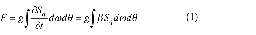
where
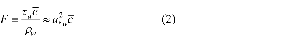
Equation (2) implies conservation of stress across the interface (subscripts a and w referring to air- and watersides, respectively), and we use
Terray et al. (1996) then used dimensionless analysis to parameterize the near surface TKEDR in terms of wave properties, as the significant wave height, Hs, and wave age
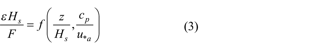
Here f is an empirical function determined from the data. They analyzed in particular
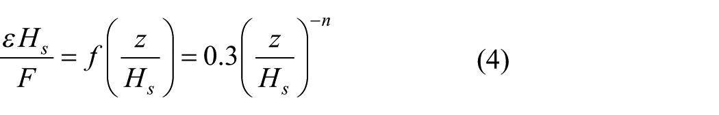
over a certain range of depths. Terray et al.’s (1996) measurements were made from arrays of three types of current meters mounted on a tower in Lake Ontario at fixed depths below the mean surface (up to 6 m depth). Their data were analyzed through Taylor’s frozen turbulence hypothesis, which consist in obtaining wavenumber spectra through simple multiplication of the frequency spectra times a mean advection velocity. For their experiment, they chose for such assumption the wave orbital velocity advected past the probes (cf. Lumley and Terray, 1983). From their results, Terray et al. (1996) proposed a layer of constant dissipation near the surface (<0.6Hs) where breaking occurs and contains half of the total dissipation, with n = 1 in equation (4); a deeper layer that depends on wave age, where n = 2; and a deeper layer that would follow the LOW. The total integration of ε in the ocean surface layer equals the wind–wave input for their experiment.
These findings were supported by the results presented by Drennan et al. (1996), who calculated TKEDR from Doppler sonar current meters mounted on a small vessel. Their measurements were made at a roughly fixed distance below surface of approximately 1.5–2 m. TKEDR was again calculated using the frozen turbulence hypothesis, but with the advection velocity represented by the mean ship speed, finding values and behavior of the TKEDR as in Terray et al. (1996).
Gemmrich (2010) used upward-looking acoustic Doppler sonar mounted on a platform, pointed to the surface, together with sensors that allowed for the detection of wave breaking. He directly calculated TKEDR through Kolmogorov theory (KT; see section “TKEDR calculations”) applied directly to wavenumber spectra, avoiding the use of Taylor’s frozen turbulence hypothesis. He also calculated the TKEDR with a second-order structure function (SOSF) method, useful when analyzing scales larger than dissipation scales (Kolmogorov, 1991; Thomson et al., 2016). Interestingly, his findings include significantly enhanced TKEDR values only directly under wave crests, while values under troughs were much lower and more consistent with LOW. He also obtained a balance between energy input and dissipation though, in the ocean surface layer. These results apparently differed from the previous research mentioned, but they coincide if different dynamical frames are taken into account (Thomson et al., 2016).
More recently, Sutherland and Melville (2015) studied the TKEDR beneath breaking waves. They combined infrared imagery with acoustic Doppler profilers to calculate dissipation rates from the surface to a depth equal to several significant wave heights. In this way, they obtained an accurate integration of the energy dissipation over the wave—affected layer. Sutherland and Melville (2015) found total integrated dissipation in the water column to be in agreement with dissipation rate values expected from young waves. They found that near the surface, the dissipation decayed as a function of depth as
They also compared results to numerical models, as large eddy simulation (LES), a popular technique for simulating turbulent flows consistent with KT of self-similarity, and to the TKEDR calculated through the structure function method. They suggested the enhanced values of TKEDR at the top layer found in previous research (as in Gemmrich, 2010) could be due to the action of microbreakers not resolved in the LES models since they were the dominant source of turbulence for those conditions. Later, though Banner and Morison (2016) showed that microbreakers would not generate enough energy as to create the high values of dissipation rates found at such depth, leaving a door still open for different solutions.
Various ideas exist today about the relationship between the dissipation rate of energy right underneath the surface and the prospective forcing affecting it: wave age, swell, sea-state, wind–wave input, microbreakers, Langmuir circulation, and other effects (Babanin, 2011; Gemmrich et al., 2016; Kukulka and Brunner, 2015; Soloviev and Lukas, 2003; Sutherland et al., 2013; Sutherland and Melville, 2015; Thomson et al., 2016). Researchers found different solutions or parameterizations, and these solutions vary depending on the frame utilized, environmental conditions, and evident differences in the experimental setup. Indeed one key element determining the differences among experiments is the instrumentation capability of measuring current turbulent fluctuations throughout the entire ocean surface boundary layer, up to the very surface. Some of the previous experiments could not reach the upper meter of the ocean (i.e. Drennan et al., 1996; Terray et al., 1996), others could point their sensors toward the surface while settled at a certain depth (i.e. Gemmrich, 2010), and fewer measured the complete oceanic boundary layer including the ocean surface (i.e. Thomson et al., 2016). In general, turbulence measurements agree with the initial findings of higher values of dissipation at the surface, decreasing in depth; the sublayers probably are separated by sea age and maybe dependent of the observation frame (Thomson et al., 2016). Still, the differences among them were the incentive for this publication.
In this context, we present a yet unpublished set of observations to supplement previous studies, eventually useful for the evaluation of alternate or classical theories. Indeed, our motivation for this article was the apparent conflicting results published in the field during the last decade about the boundaries of the wave-influenced surface layer and the expected vertical structure of energy dissipation rates within it. This work intends to present a description of new data, to contribute to the few experiments in open ocean, available up to date.
We investigated the relationship between wave phase and TKEDR in the upper layer of the ocean in the Labrador Sea during summer 2004. The area was selected as a key area for dense water formation, and for the particular biochemical characteristics present during spring and summer, when a phytoplankton bloom usually occurs. A one-dimensional (1D) Doppler sonar was mounted on an air–sea interaction spar (ASIS) buoy (Graber et al., 2000), to obtain measurements of horizontal current variability at about 1.8 m depth, together with other sensors, aimed at study of the oceanic boundary layer and the few upper meters of the ocean. We present here the analysis of the 1D current speed variability during the experiment, its spectra, and the TKEDRs calculated through the KT (Kolmogorov, 1941). We focus on the effects of wind and waves on the dissipation rates and on their possible dependency on wave phase. We also consider the possible flow distortion triggered by the supporting platform.
As in previous experiments mentioned in the literature (cited above), our experiment is also based on the use of coherent sonar Doppler radar to measure turbulent fluctuations and the study of the dissipation rates at the ocean surface layer. However, they differ in the depth of the sensors, the setup of the experiment (on a tethered buoy in a lake or open ocean vs fixed towers or towed sensors), the frequency of the sensor utilized, and the method used for the TKEDR calculations (k-spectra vs f-spectra, structure functions, correlations, etc.). These differences appear as the most important factors to consider when comparing TKEDR results, and their relative importance is explained further on.
Breaking and nonbreaking waves add turbulent energy into the surface layer (Babanin, 2011). The energy derived from waves and mixed into the upper layer is implicitly included in our calculations, as our measurements were obtained within the surface wave-influenced layer, that is, at depths around 1.8 m. Considering that the wind conditions during the Labrador Sea experiment were moderate (around 10 m/s or less), the assumption that wave breaking in open ocean will occur less than 5% of the total surface waves seems appropriate for our case, as demonstrated by Zhang (2008) and Zhang et al. (2009), among others.
Particular attention was directed here toward the accuracy of the measurements by analyzing the potential flow distortion induced by the platform. While wind distortion effects due to the experiment settings on board vessels (Oost et al., 1994; Pedreros et al., 2003) and other platforms; O’Sullivan, 2013 have been thoroughly studied, little information is available about the flow distortion induced by the presence of a platform over current fluctuations (see Sutherland and Melville, 2015: Appendix C). A detailed study of wind and current distortion induced by the platform in the current experiment (and others) appears in Gremes-Cordero (2010). Here, we will refer only to those results related to the present research.
In the following, details on the experiment and instrumentation are presented in section “The Labrador Sea experiment,” followed by a description of the methods and post-processing utilized (section “Methods applied”). The TKEDR results are discussed in section “Discussion of the results,” followed by the conclusions in section “Conclusion and summary.”
The Labrador Sea experiment
The primary goal of the Labrador Sea experiment was to investigate the air–sea flux of carbon dioxide during a typical plankton bloom occurring in the Labrador Sea in the summer (Strutton et al., 2011). An ASIS buoy instrumented to measure oceanic and atmospheric variables at the surface boundary layer (Graber et al., 2000) was deployed near 53°N, 49°W in June 2004 (Figure 1). The variables targeted were wind speed, wind stress, air and sea temperatures, surface waves, upper ocean turbulence and mixing, and parameters related with CO2 concentration in both media and the transfer of it across the surface. Here, we focus on the oceanic turbulence, the TKEDR, and their relationship with surface physical processes.
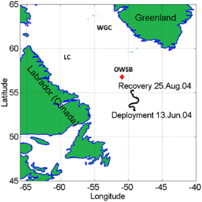
The site of the ASIS deployment and its path after 10 days.
The main hydrographic conditions during the experiment have been well detailed in Martz et al. (2009), presenting winds ranging from ~1 to 15 m/s with a mean of 6.3 ± 3.1 m/s during the period studied (Figure 2). The experiment was conducted between 13 June and 25 August, but since the buoy was set adrift 10 days after the starting of the experiment, only those first 10 days during which calibration settings were consistent, and the wind was strong enough to keep ASIS pointed in a favorable direction for accurate data measurements, were analyzed here.
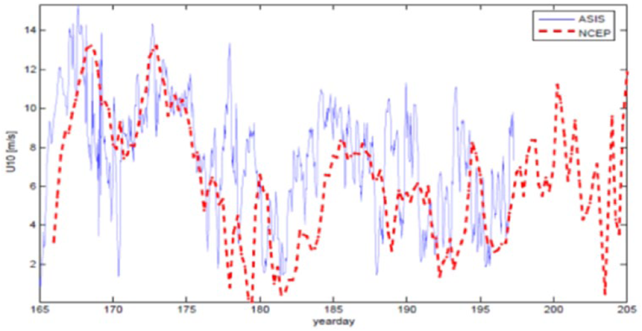
Mean wind values from the ASIS tower in blue and from National Centers for Environmental Predictions (NCEP) 4-hour reanalysis data interpolated to 0.5-hour intervals in red.
This research is focused on the turbulent current variability obtained from a 1D pulse-to-pulse coherent Doppler sonar, the DopBeam. The outward-pointing sonar was mounted on ASIS, at about 1.8 m below the mean water line, to measure horizontal (radial) current fluctuations (Figure 3).
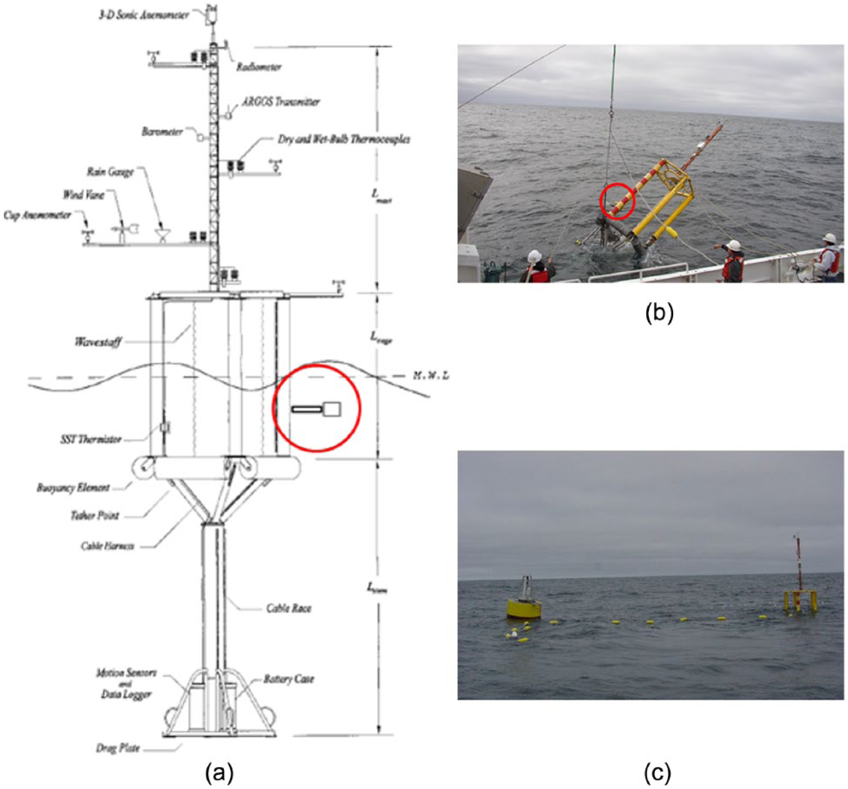
(a) ASIS schematic diagram (adapted from Graber et al., 2000): note that DopBeam was not mounted on the original buoy, but it is indicated in the plot (red circle) to show the relative position. (b) ASIS during deployment, with the red circle indicating the 1D DopBeam sonar about 1.8 m under the upper frame. (c) ASIS with the tether that allows it to follow the surface displacements.
The ASIS buoy
The ASIS platform is an easily portable and deployable buoy system capable of high-resolution measurements of waves and atmospheric fluxes. Its design has a mechanical response that reduces the motion of sensors relative to the surface, while retaining the low flow disturbance characteristics of a slender spar buoy, allowing for high accuracy mean and flux measurements in the air and water (Graber et al., 2000).
To avoid downward forces that can be generated by connecting the spar to a subsurface anchor, the ASIS was attached to a surface mooring (the “tether buoy”) by means of a buoyant tether made of wire rope and a coil chain with plastic floats, to keep it at the surface. The influence of the mooring pull is a key parameter and was extensively studied by Anctil et al. (1994), Graber et al. (2000), and others.
The use of a surface mooring has other advantages as the ability to carry subsurface instrumentation such as current meters, acoustic Doppler current profilers (ADCPs), ambient noise sensors (e.g. wind observation through ambient noise (WOTAN)), and thermistor strings (Figure 3). This arrangement also facilitates launching and recovery operations (Graber et al., 2000).
Measurements obtained from the sensors mounted on the ASIS must be transformed into fixed coordinates. The parameters of the buoy motion are provided by a 6-degree-of-freedom inertial package consisting of “strapped-down” orthogonal triplets of accelerometers, angular rate gyros, and compass. By measuring both the motion of the buoy and the position of the surface relative to it, the need to control or have a priori knowledge of the response function of the platform is avoided. An array of eight wave height gauges within the pentagonal “cage” of the ASIS provide measurements of surface elevation and allows for the calculation of the wave directional spectra. For a detailed description of the ASIS and its equipment, see Graber et al. (2000), and for our experiment configuration details, see Martz et al. (2009).
The Doppler sonar and its data
The pulse-to-pulse coherent Doppler sonar utilized in this experiment works similar to the most widely used incoherent Doppler sonar. The main difference being the transmission of a series of identical pulses and to use the phase shift in between those pulses for the calculation of the velocities (L’Hermitte and Serafin, 1984). There are basically two types: a sonar capable of measuring the three components of the velocity fluctuation (three-dimensional (3D)), as the marine acoustic velocimeter (MAV) does, and the ones measuring just the radial component in the direction of the transmitter (1D). We present here the analysis of the data obtained with the latter, a unidirectional sonar called Miami DopBeam (L’Hermitte and Haus, 1999). The Miami DopBeam is a self-contained Doppler sonar, based on the data acquisition system manufactured by SonTek, Inc.
The pulse-to-pulse coherent unidirectional Doppler profiler measures the backscattered signal phase change associated with target motion between sets of pulses at a very high sample rate (468 Hz) and at densely spaced locations. It is possible to transform those recorded phases into velocity fluctuations (Veron and Melville, 1999), and because of the spatial proximity of the measured points (0.8 cm), we can perform a direct calculation of the wavenumber spectra avoiding Taylor’s assumption or frozen turbulence hypothesis. This approach reduces error in the TKEDR calculations avoiding the difficult task of choosing the correct transform velocity when converting from the frequency domain to the wavenumber domain (i.e. Ardhuin and Jenkins, 2006).
There are certain limitations for the use of this coherent Doppler sonar, as the availability and movement of the targets bound the backscattered signal. However, previous studies together with the present work prove this a weak limitation. The DopBeam was successfully tested in laboratory experiments, coastal shallow inlets, and lakes, showing its capability to resolve wavenumber spectral levels in the ISR (Gargett, 1994; L’Hermitte and Haus, 1999; L’Hermitte and Serafin, 1984; Veron and Melville, 1999), as well as in oceanic conditions (Gemmrich, 2010; Gemmrich and Farmer, 2004). For this reason, it has been considered an ideal instrument for measuring turbulence and energy dissipation in the upper layers of the ocean, within the wave-influenced oceanic boundary layer (Veron and Melville, 1999).
The Miami DopBeam is capable of measuring closely spaced bins (0.8 cm), for a total distance of 150 cm. It can record backscattered acoustic signals during 20 minutes on the hour, which are actually phase fluctuations comprised between −π and π (Figure 4).
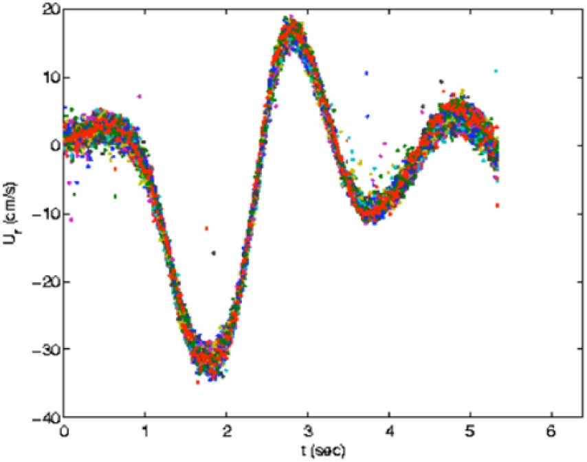
An example of the radial velocity time series, for 17 June, at 04:00 UTC. The colors denote different bins, that is, distance from the sensor.
The sonar stores this information into two types of files: one type suitable for mean current calculations and the other fit for variability calculations, depending of the time steps averaged before the storage. In this work, only the second type of files with sampling frequency of 96.4 Hz rate were utilized for the calculations.
Methods applied
The first step for our calculations is to unwrap the signal from the radar view (−π and π) to a regular time series, eliminating ambiguity and overlapping. Then, the phase’s time series are transformed to velocity fluctuations following Veron and Melville (1999). A preliminary quality control help disregard data with excessive noise. Furthermore, the velocities are transformed to geolocation coordinates, to be compared with winds and other variables. A flow distortion quality control is then applied as described in section “Flow distortion assessment.” Only after these verifications, the wavenumber spectra of the velocity fluctuations are calculated, and the Kolmogorov method is applied to obtain the TKEDR. Spectra were also averaged in time and space at different intervals, to test for order of magnitude and the applicability of the method to our dataset. For more details in the procedure, we refer the reader to Gremes-Cordero (2010).
TKEDR calculations
The calculation of TKEDR followed KT of turbulent energy cascade, by assuming that there is a portion of the spectra where energy is only transmitted from large-sized eddies to smaller ones without any external input of energy (Kolmogorov, 1941). In this portion, called the ISR, the rate of dissipation of such energy (ε) can be defined as

where
Many studies had been conducted in order to find a suitable value for the constant D (Gibson, 1962; Hinze, 1959; Phillips, 1977; and others). More recently, the value of the constant had been adapted to environmental conditions and laboratory experiments (Gemmrich and Farmer, 2004; Veron and Melville, 1999). We followed here the Hinze (1959) approach as Drennan et al. (1996) and Veron and Melville (1999), who considered for ISR
where
After calculation of the wavenumber spectra, we detected the ISR by fitting a line with slope
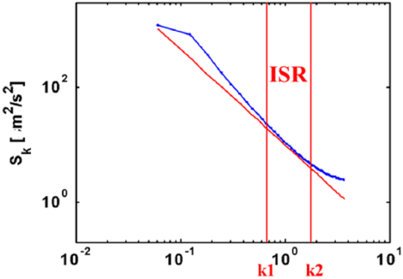
Schematic representation of the calculation of ε from the velocity wavenumber spectra. The inertial subrange (ISR) determined as the portion of the spectra that fits the red line with slope −5/3 is delimited by the wavenumbers k1 and k2 (red vertical lines).
Note that using only the portions where an ISR exists for our calculations, we do not consider the moment of breaking, as the theory itself does not contemplate the input of energy, by definition of ISR. We assume that measurements are taken right before or immediately after the wave breaks, with enough time as to reach stationary conditions again.
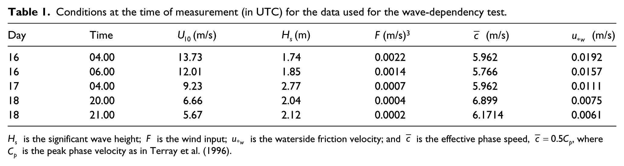
Initial tests were performed over several files, averaging time steps between 1 second and 1 minute, to check the order of magnitude of the dissipation rates and the effects of flow distortion. The environmental parameters calculated for the files chosen for the present analysis are presented in Table 1.
Conditions at the time of measurement (in UTC) for the data used for the wave-dependency test.
Parameterization of wave effects
To introduce the effect of waves, we scaled the TKEDR with the significant wave height (Hs) and the momentum input
Note that the TKEDR values presented here were calculated during moderate wind conditions (mean average of approximately 9 m/s). The data obtained in low wind conditions (i.e. <5 m/s) are considerably noisier, allowing only a shorter part of the available data to be analyzed.
Flow distortion assessment
Careful attention was made to minimize and quantify any effects of flow distortion in the turbulence measurements, which ultimately could affect the TKEDR values. First, we differentiated the periods when the DopBeam was in front of ASIS with respect to the mean flow (i.e. when not in the wake of ASIS). Since yaw, pitch, and roll were recorded throughout the duration of the experiment for motion corrections, we have the absolute position of the ASIS with respect to the magnetic North. We also had the 3D current velocities recorded from a 300-kHz ADCP mounted at 13 m depth on the ASIS. We performed then a comparison between the position of the buoy and the ocean currents, with positive angles indicating that the currents are coming toward the buoy and negative angles receding from it. We calculated the wavenumber spectra for the optimal range of the DopBeam, that is, where the signal-to-noise ratio is expected to be maximum (from bins 10 to 137 = 16 to 118 cm). Figure 6 indicates values of TKEDR coming toward the ASIS (blue dots) and away from it (red crosses).
Values of TKEDR (ε) differentiated according to the prevailing flow direction. Blue dots denote flow coming toward the DopBeam; red crosses are ε with flow approaching from behind the instrument. Note that red values have not been used in the successive analyses.
Second, since flow distortion is expected to decrease significantly moving away from ASIS, the DopBeam data were analyzed by looking separately to the turbulent fluctuations at different distances from the ASIS leg, that is, from the sensor. Three datasets of TKEDR were then created: values calculated from bins at 16 to 118 cm just mentioned, another from 10 to 73 cm from the sensor, and the last one from 80 to 143 cm away. If the ratio of turbulence estimates was significantly different from 1, the data were considered to be distorted by the ASIS platform and were hence rejected. In particular, it was determined that the best signal-to-noise ratio was found for the bins 62–134 (approximately 72–134 cm from the receiver), that is, far enough away from the flow distortion induced from the platform, but close enough for the actual signal to be robust. For extensive details on the procedures and examples, see Gremes-Cordero (2010).
Wave-phase dependency
In addition to the previous calculations, the values of TKEDR below wave crests and troughs (both defined from simple observation of the time series) were also recorded (Figure 7). After observing several files, we determined that most of the crest and troughs lasted about 15 time steps (0.1 second approximately), and we set such limit as a boundary for each crest or trough (Figure 8).
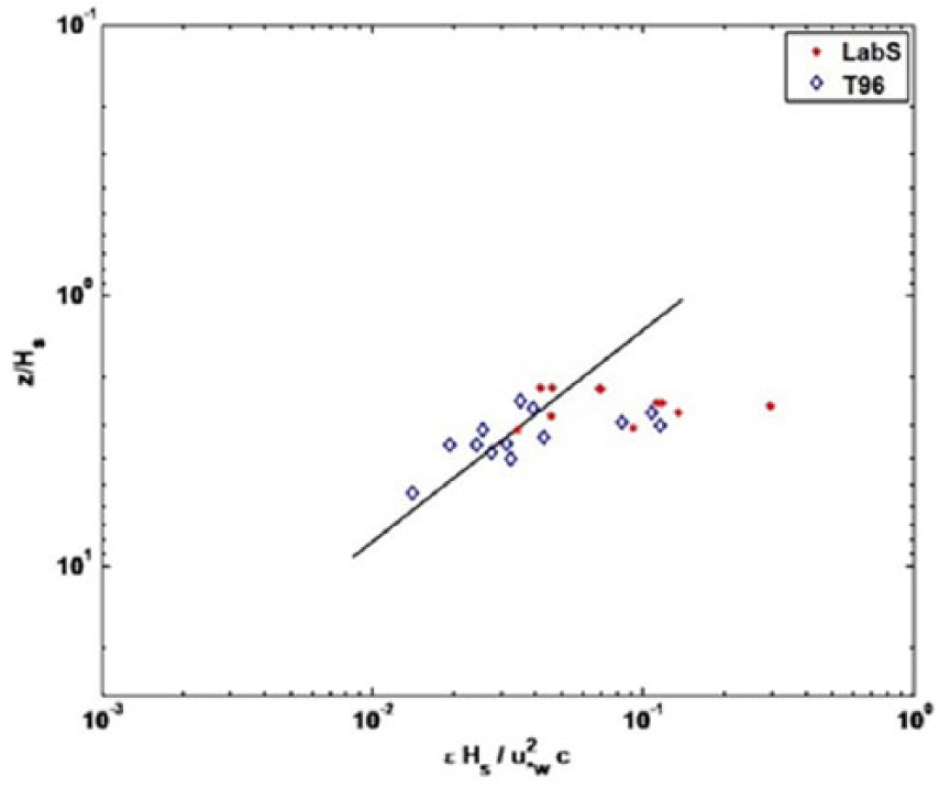
TKEDR with the scaling of Terray et al. (1996). The data were obtained between 16 and 18 June 2004 (corresponding to Table 2). Blue diamonds correspond to Terray et al. (1996) data for horizontal fluctuations; the red asterisks are the results of the Labrador Sea experiment, also for radial TKEDR (ε), and the black line is the regression fit.
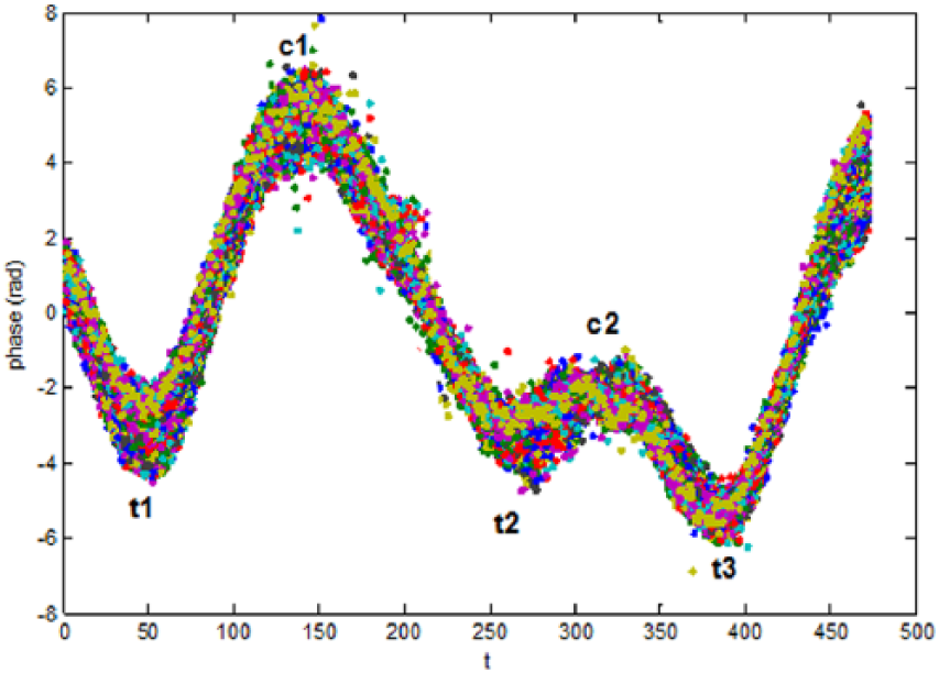
Phase signal in function of time, with differentiation of crest (c) and troughs (t). The colors denote the different bins. The time steps represent 1/96 Hz. The example is for 16 June at 4:00 GMT.
We proceeded then with two different approaches: once determined the 15 time steps that delimit a crest (or trough), we calculated the 15 corresponding wavenumber spectra, one for each time step, along the optimal range determined before. Then, we averaged them and calculated one TKEDR from that averaged spectrum. The other approach involved the calculation of one TKEDR from each of the 15 spectra, obtaining then the final value from the average of all those 15 TKEDRs. The difference between the TKEDR obtained through these two methods was smaller than 0.3%. The second option was preferred for our analysis, as it allowed us to check the magnitude and accuracy of each value of TKEDR as we proceed. Note that among the 15 spectra, only the ones with a clearly defined ISR were used to calculate the TKEDRs, as required by the Kolmogorov method. We also obtained TKEDR for intermediate points, to find the same results: only small changes in TKEDR values, with the same order of magnitude.
Statistical analysis
Once the values for crests and troughs were obtained, a simple statistical analysis was performed. The unpaired T-test compared the values of TKEDR for crests and troughs, considering the hypothesis of similarity, that is, the similarity between two groups is proved when the p-value is >0.05. The p-value is the probability that the observed result is not related to the one compared to. We can observe in Table 2 that all the p-values are larger than the threshold of 0.05, proving that the differences between crest TKEDR and trough TKEDR are not significant, that is, the hypothesis of similarity, with a 95% confidence, has been proved.
Subset of TKEDR analyzed for wave dependency, for days 16–18 June 2004.
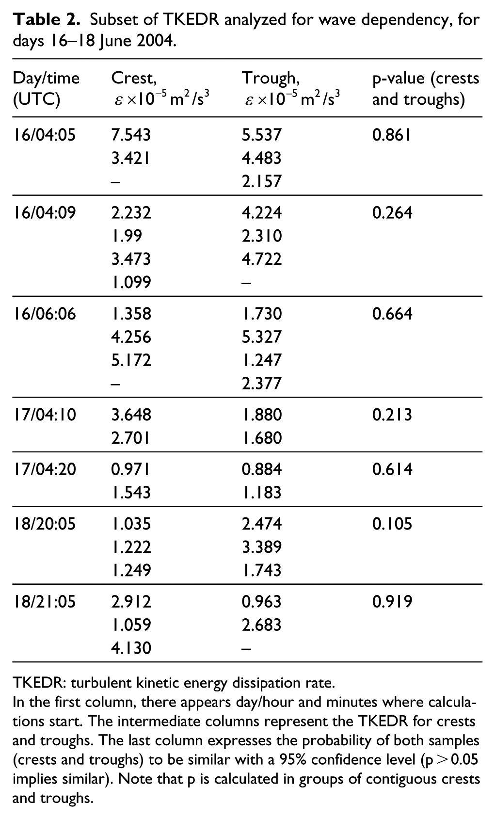
TKEDR: turbulent kinetic energy dissipation rate.
In the first column, there appears day/hour and minutes where calculations start. The intermediate columns represent the TKEDR for crests and troughs. The last column expresses the probability of both samples (crests and troughs) to be similar with a 95% confidence level (p > 0.05 implies similar). Note that p is calculated in groups of contiguous crests and troughs.
Discussion of the results
Our calculations give values of TKEDRs comparable to previous research, that is, approximately two orders of magnitude larger than the LOW dissipation rates are (Drennan et al., 1996; Sutherland and Melville, 2015; Terray et al., 1996; etc.). This is an expected result in the surface oceanic boundary layer (SOBL) and proves the capabilities of the instrument for open-ocean conditions.
Following the scaling of Terray et al. (1996), our scaled TKEDRs show good agreement with the values presented by Terray et al. (1996), as shown in Figure 7. Note that the apparent order of magnitude difference within the maximum and minimum values is related to the different conditions at the time of the measurement, as wave height and wind speed (see Table 1). In other experiments, the TKEDRs were calculated consecutively in time, and the experiment conditions do not change considerably within, for example, 1 minute. In this figure instead, our values belong to measurements obtained at different hours or even days, with very different winds and currents.
We also scaled our TKEDR as in Gemmrich (2010), finding an average scaled TKEDR
Moreover, the input of the wind forcing
Differences in the experimental settings are key for more than one variable. First, the depth of the sensor establishes the layer to be probed, the upper wave-breaking influenced layer or the lower layer with constant dissipation rates, varying then their order of magnitude. Second, it establishes the reference frame for the measurements, which implies defining the range of values for TKEDR, larger in a follow frame than in a fixed frame (Thomson et al., 2016).
Gemmrich (2010) obtained measurements with a sonar pointing to the surface and has a sampling rate of 100 Hz that helped avoid bubbles and reverberation of the signal. Terray et al. (1996) obtained measurements with a sensor mounted on a tower, at a fixed depth. The sensors in the Drennan et al. (1996) experiment, instead, were mounted on a small vessel, so measurements were made at a roughly constant depth below the surface and above Terray et al. (1996) measurements. The values among these experiments were consistent. In our case, the experiment settings can be defined as intermediate between the previous: while the ASIS buoy is tethered to the anchored part, allowing it to freely move with the surface, the depth of the sensor is about 1.8 m, roughly the same depth of Drennan et al. (1996) measurements. Note that our instrument is also capable of distinguishing between crests and troughs, a remarkable limitation in the Terray et al. (1996) experiment. We showed that our TKEDRs do not exhibit a dependency on wave phase, pointing out a probable mixed up energy within the layer considered. This supports the idea of an internal sublayer where the energy of wave breaking can be discerned from the total background turbulence, as pointed out by Thomson et al. (2016). Under these considerations, one assumes that Terray et al. (1996) and Drennan et al. (1996) missed the large TKEDR of the crests, measuring only the lower values of troughs. The present analysis is intended to add other results to compare.
Sutherland and Melville (2013) proposed another explanation for the discrepancy in TKEDR values between Terray et al. (1996) and Gemmrich (2010). They obtained measurements throughout the whole layer affected by waves and showed that the total integrated TKEDR is related to the breaking of young waves, while “old” waves will not produce the same effects. This can tie both previous measurements together, pointing to the age of waves as a main effect over turbulence dissipation rather than the breaking effects.
Thomson et al. (2016) obtained observations of turbulence in open ocean and compared them to numerical models and previous assumptions and found that TKEDR values depend rather on the reference frame than on the wave phase. They also determined that the energy introduced by wave breaking is equal to the integration of the TKEDR in depth when the wind is lower than 15 m/s, which also validates our results.
Hence, the environmental conditions (wind speed, fetch, etc.) seem to play a more important role in the TKEDR parameterization than one would prefer for a correct parameterization. While the different frames would explain differences in the TKEDR order of magnitude, they might not solve the problem of uniformity in the calculations as the different sensor depth would. Hence, we also propose other two factors not considered in previous research, as contributory to the different outcomes: the flow distortion effects induced by the platform, and the different methods utilized for the TKEDR calculations.
Obvious differences in flow distortion will appear from a floating semi-free device than from a fixed tower or fixed instrumentation. As to the best our knowledge, there is no available literature showing an algorithm proved to effectively correct this type of distortion, and we presented here a novel empirical approach (see section “Flow distortion assessment”) that opens the doors for future research. In our case, the influence of the platform was detectable, and it could be responsible for the uniformity of the TKEDR found. To verify this assumption, other ASIS deployments are needed in the light of this new evidence.
Finally, the different methods used for TKEDR calculations could potentially contribute to some of the variability. Some of the authors aforementioned used Taylor’s approach of frozen turbulence, which has a vital dependency on the transport velocity assumption (Shet et al., 2017; Squire et al., 2017). Here, we avoid the Taylor’s hypothesis by obtaining directly wavenumber spectra and TKEDR through KT. Gemmrich (2010), Sutherland and Melville (2015), and Thomson (2016) utilized the structure function for the calculations, a useful tool when considering anisotropy. There is evidence of similar TKEDR results obtained with the Kolmogorov method and with the SOSF for high Reynolds numbers and for the ISR part of the spectra (Constantin et al., 1999; DeSilva et al., 2015; McMillan et al., 2016). Coincidentally though, Gemmrich and Thomson experiments measure the variability of the vertical current, while we are measuring the horizontal turbulent component. Could some discrepancy arise from an anisotropic variability? Could this anisotropic turbulence derive from the flow distortion created by the platform? More research in the topic is required to solve these quizzes, by comparing spectra of the three components of velocity fluctuations.
Conclusion and summary
We calculated TKEDR at the surface layer of the open ocean by means of a coherent Doppler radar mounted on an ASIS buoy, deployed on the Labrador Sea during summer 2004. ASIS is particularly suited to measure the exchange of properties between air and ocean with enough frequency as to determine turbulent fluctuations (Graber et al., 2000). The data presented here were obtained with the 1D DopBeam, a coherent pulse-to-pulse sonar that measures phase signals at very closely spaced bins (0.8 cm).
The proximity of the bins allowed for the direct calculation of wavenumber spectra, to obtain TKEDRs according to the KT. The wave effects were introduced in our calculations by adopting Gemmrich et al. (1994) and Terray et al. (1996) parameterization, which takes into account the wave-phase velocity to determine the input energy from wind and waves.
Our TKEDR values are in good agreement with the Terray et al. (1996) and Drennan et al. (1996) values found previously and with some recent measures and similar (but not identical) conditions, for example, Thomson et al. (2016), Sutherland and Melville (2015), and so on. Such agreement proves the broad applicability of the method and the accuracy of the measurements.
Noticeably, no TKEDR dependency on the wave phase was found in the present experiment, which differs from some other research, as is the case with Gemmrich (2010). We explained these differences as derived from some key elements of the experiments: the depth of the sensors, the type of platform and its consequential type of dynamical frame, the flow distortion induced by the platform, and the method used for the calculation of TKEDR. Anisotropy in the turbulent components could potentially influence the comparison among experiments.
Thoughtful consideration was given here to the influence of the platform in the dissipation rate calculations, an element often disregarded in previous experiments. The optimal range in function of distance from the platform was determined empirically by quantifying the noise at the receiver. Such approach allowed for a reduction in the spectral noise and assured the accuracy of the TKEDR calculated. An algorithm to determine the best accuracy in various situations is still needed and is the subject of our present research.
In summary, the quantitative analysis performed over this data provides new ground for studies of turbulence in the upper ocean. In addition to the main goal of establishing a possible dependence of TKEDR with wave phase, our calculations were useful to assess the correspondence of our values with previous findings and to determine the signal-to-noise optimal ratio.
Footnotes
Acknowledgements
I gratefully acknowledge the invaluable contributions of Tripp Collins to an earlier version of this manuscript. I also thank Will Drennan for his scientific guidance and financial support during this research and J. Gemmrich and H. Potter for helpful commentaries that greatly improved this article. I thankfully acknowledge Mike Rebozo, Joe Gabriele, and Dr Hien Nyugen’s assistance with the technical operations, as well as the captain and crew of the R/V Endeavor.
Declaration of conflicting interests
The author(s) declared no potential conflicts of interest with respect to the research, authorship, and/or publication of this article.
Funding
The author(s) disclosed receipt of the following financial support for the research, authorship, and/or publication of this article: This work was funded by NSF OCE-0327271.