Sage Journals: Discover world-class research

Abstract

Tidal inlets get disconnected depending on the seasons due to the formation of sand bars near its mouth are termed as “seasonally open tidal inlets.” These inlets are usually small of width of about 100 m and occur in micro-tide (tidal range not exceeding 1 m). Since the east coast of India experiences a net littoral drift of up to about 0.8 Mm³/annum, which is one of the largest in magnitudes that needs to be considered in the analysis of modeling of the sand bar formation and the associated phenomena. Kondurpalem inlet situated along the South east coast of India is considered as a case study. A frequency domain wave model (STeady-state spectral WAVE) has been used to compute the nearshore wave climate. The wave-induced currents have been obtained, and the longshore sediment transport rate is obtained through empirical relations. The tidal prism is found from measured depth and tidal velocity by solving shallow water equations. The stability of the inlet is investigated by applying the criteria developed by Bruun (1986). The effect of a pair of training walls on maintaining the stability of the mouth is reassessed over the periods.

Keywords

Sediment transport inlet stability tidal prism longshore velocity longshore drift

Introduction

Seasonally open tidal inlets close every year during lean/calm periods due to the trapping of longshore drift leading to the formation of sand bars across their entrances. These inlets are usually small (inlet width: ~100 m) and occur in micro tide-wave dominated coastal environment, where seasonal variation in the stream flow and wave climate are experienced. Davies (1964) classified shorelines based on the prevailing tidal range. Hayes (1979) re-defined the classification of Davies (1964) based on the tidal range as a function of mean wave height. The mouth of micro-tidal inlets get closed to the ocean over a number of months annually due to the formation of sand bars across their entrances, usually during summer when the stream flow is low and long-period swell waves dominate, or when longshore transport rates are high. Many of these inlets are navigable provided, the formation of sand bar can be avoided or minimized. The seasonal closure of inlet leads to two main problems: first, the ocean access for boats gets limited and second, the water quality in the lake/estuaries/lagoon will deteriorate during the months of inlet closure. A brackish water lake rich in flora and fauna can deteriorate in quality due to sand bar formation which can lead to drastic reduction in the fish catch. Hence, there is a need to keep the inlet permanently open to have year-around navigability and to improve the flushing of the lake/estuaries/lagoon. Bruun (1986) considered several inlets around the globe with the minimum depth in the inlet gorge being 4.5 m and the maximum depth being 18 m. These inlets were located in semi-diurnal tidal regimes, with a spring tidal range of about 3 m. The work included 12 inlets along the Indian coast through a detailed survey and observation during the monsoon and off-monsoon season. Ranasinghe and Pattiaratchi (1999) have developed a morphodynamic model for the simulation of longshore, cross-shore sediment process and validated for the inlet stability for idealized conditions. Thanh et al. (2012) compared the cross-sectional stability between empirical and numerical approach. The relation between the cross-sectional area and the tidal prism was considered. Kraus (1998), Suprijo and Mano (2004), and Van de Kreeke (1998, 2004) considered other parameters like tidal cycle period, tidal velocity, channel width, and longshore sediment transport rate in discussing about the stability of tidal inlets. Therefore, it is necessary that a proper understanding of the process causing inlet closure is imperative for finding working engineering solutions for this problem. One way to achieve this would be to undertake continuous and long-term field measurements which would be time-consuming and highly uneconomical.

Study area

In this study, Kondurpalem inlet which is one of the several inlets that sustain estuarine ecosystem of Pulicat Lake has been chosen. Pulicat Lake is located at 60 km from north of Chennai city which is the second largest—brackish water—lake in India. The study area Kondurpalem inlet, (14°01′07″ N, 80°09′24″ E) Andhra Pradesh (shown in Figure 1(a)), is along the east coast of India. From Figure 1(b) and (c), it is observed that the inlet is active in May 2008 and closes in October 2009, indicating that the inlet being dynamic in nature. It straddles the border of the two maritime states of Tamil Nadu and Andhra Pradesh along the south east coast of India. The barrier island of Sriharikota separates the lake from the Bay of Bengal. The average depth of water has reduced from 1.5 to 1 m.

Figure 1.

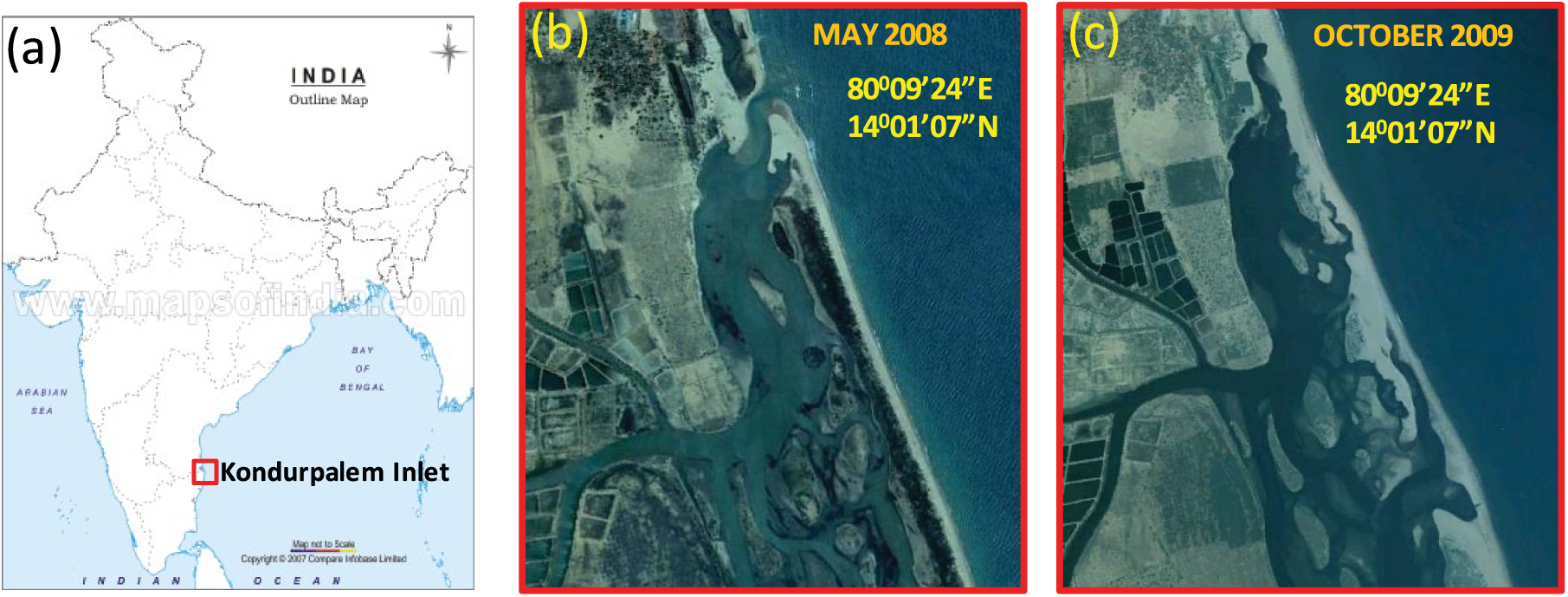
Study area Dynamic nature of inlet.

Methodology

The detailed methodology involves the collection of offshore bathymetry, wave climate, and sediment characteristics through field measurements. The measured data were used in understanding the nearshore hydrodynamics, tidal flow, littoral drift, and morphology. The schematic and detailed numerical modeling approach is shown in Figure 2.

Figure 2.

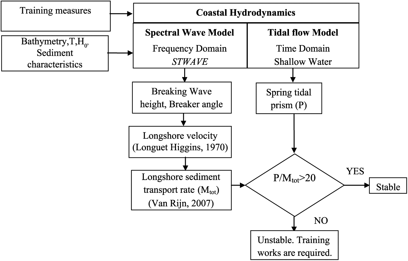
Schematic representation of modeling approach.

The measured bathymetry of the nearshore and backwater region is shown in Figure 3. It is seen that the nearshore area of Kondurpalem inlet has almost parallel bathymetry with an average slope of 1 in 115 (m = 0.0086, where m is the beach slope). The backwater area has depths up to 3 m, with an average of about 1.75 m. It is observed that the breaking of waves normally happen within a water depth of 5 m during most of the time. The breaker line is about 200 m away from the shoreline. The average slope of the surf zone is 1 in 40. The nearshore bathymetry from shoreline to 14-m water depth is used for modeling the waves using spectral approach/frequency domain approach. The entire bathymetry of the study area, including nearshore and backwater areas, is used for modeling the tidal hydrodynamics. The locations of measurements of nearshore waves and currents are shown in the earlier figure. The wave data were measured during the months of June, July, and December for monsoon months. For the other months in the absence of measured data, the derived wave characteristics from the National Institute of Oceanography (NIO) (Chandramohan et al., 1991) wave atlas have been used for deriving the wave characteristics as shown in Table 1.

Figure 3.

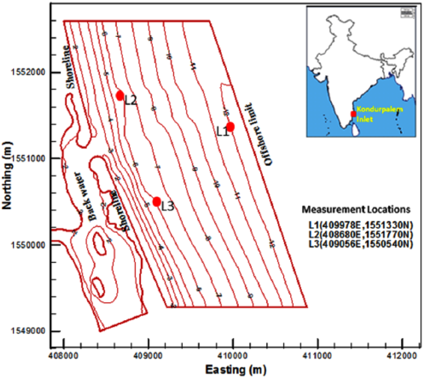
Bathymetry of the study area.

Table 1.

Offshore wave climate and wave climate derived at 12 m.

Month	Deep water wave characteristics from NIO wave atlas			Derived water wave characteristics at 12 m
Month	H_s	T_p	θ_SN	H_s	T_p	θ_SN
January	1	6.5	36	1	6.5	6
February	1.1	6	47	0.6	6	11
March	0.8	5.5	55	0.7	5.5	25
April	1.3	5.5	83	0.6	5.5	53
May	1.4	6	95	1	6	65
June	0.9	5.9	80	0.8	5.9	58
July	1.2	6.7	79	0.9	6.7	62
August	1.5	6.5	94	1.1	6.5	64
September	1.3	6.5	94	1	6.5	64
October	1.8	5.5	42	0.5	5.5	12
November	1.5	6	36	1	6	−7
December	1.1	6	80	0.9	6	−11

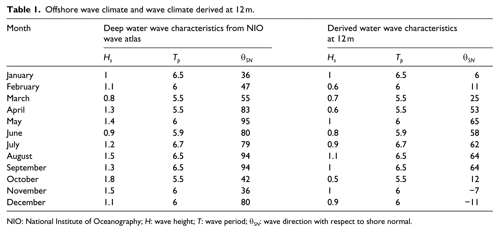
NIO: National Institute of Oceanography; H: wave height; T: wave period; θ_SN: wave direction with respect to shore normal.

A frequency domain approach has been followed, to obtain the nearshore wave climate which is strongly influenced by the variations in the bathymetry, water level, and current. The model STeady-state spectral WAVE (STWAVE), is used to simulate the depth-induced wave refraction and shoaling, current-induced refraction and shoaling, depth- and steepness-induced wave breaking, diffraction, and wind-wave growth. The input to the model is a spectrum that describes the distribution of wave energy as a function of frequency and direction (two-dimensional spectrum). The measured significant wave characteristics from the offshore location (L1 in a water depth of 12 m) are input spectrum for the propagation over the measured bathymetry for the wave simulation, for the month of July and December, 2011. The significant wave height thus simulated has been compared with the measured significant wave height in the nearshore locations L2 and L3 (both in 6-m water depth). The significant wave height thus simulated has been compared with the measured significant wave height in the nearshore locations L2 and L3 in Figure 4(a) and (b), respectively. The simulated results agree well with the measured wave characteristics for the month of July, 2011. Since, all measurements (361 numbers of H_s) are compared, this is carried out only for July by executing the spectral model, 361 times.

Figure 4.

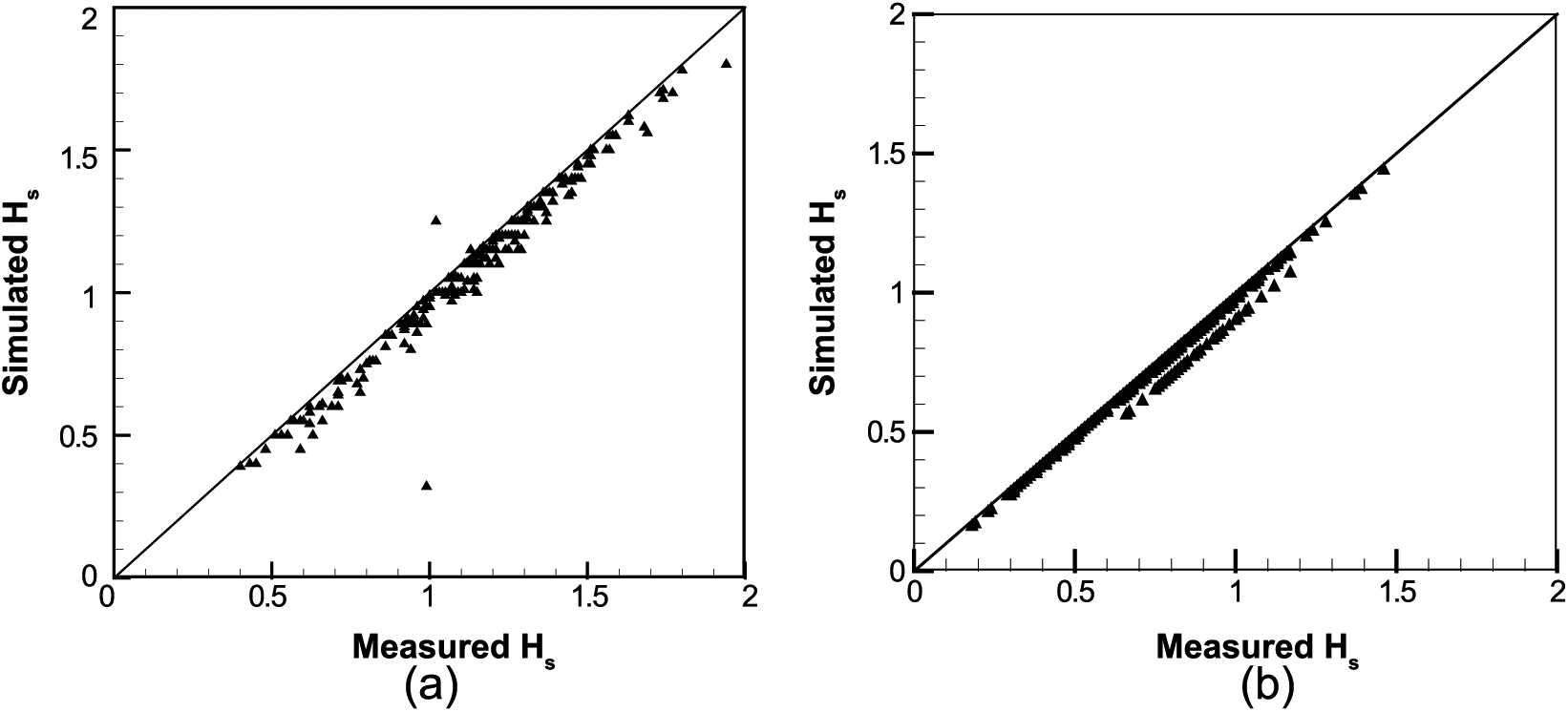
Comparison of measured and simulated wave height at: (a) location L2 and (b) location L3.

Komar Distribution method

The longshore current is computed (Longuet-Higgins, 1970) by equating gradient in the radiation shear stress to bottom friction, with assumption that the shallow water theory is valid as far out as the breaker line where the depth d is equal to h_b, the mean longshore current (V_o), in the absence of horizontal mixing

V_{0} = \frac{5 π}{16 C_{f}} γ {(g d_{b})}^{(1 / 2)} ε^{2} m (\sin α_{b})

(1)

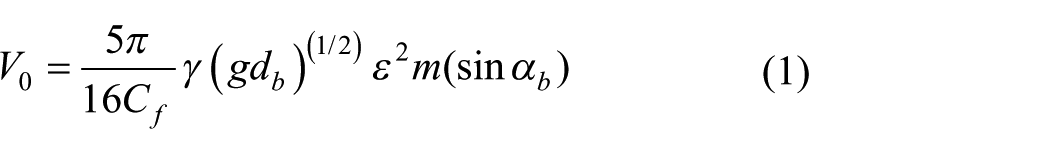
where m is the bed slope, C_f is the current friction factor (around 0.01; Longuet-Higgins, 1970); g is the ratio wave height and water depth and ε = 1/(1+0.375γ²).

However, in the real sea conditions, the propagating wave will be of random in nature and hence, there will be a lateral mixing due to different waves with varying period breaks consecutively. Hence, he proposed a solution as

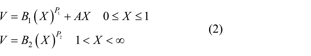
\begin{array}{l} V = B_{1} {(X)}^{P_{1}} + A X 0 \leq X \leq 1 \\ V = B_{2} {(X)}^{P_{2}} 1 < X < \infty \end{array}

(2)

where X and V are in non-dimensional form and X = (x/x_b), x is the distance normal to the shoreline, x_b being the distance from the shoreline to the breaker zone and V is the proportionality coefficient obtained with the inclusion of lateral mixing, needs to be multiplied with V₀ to obtain the actual velocity.

The other parameters are given by

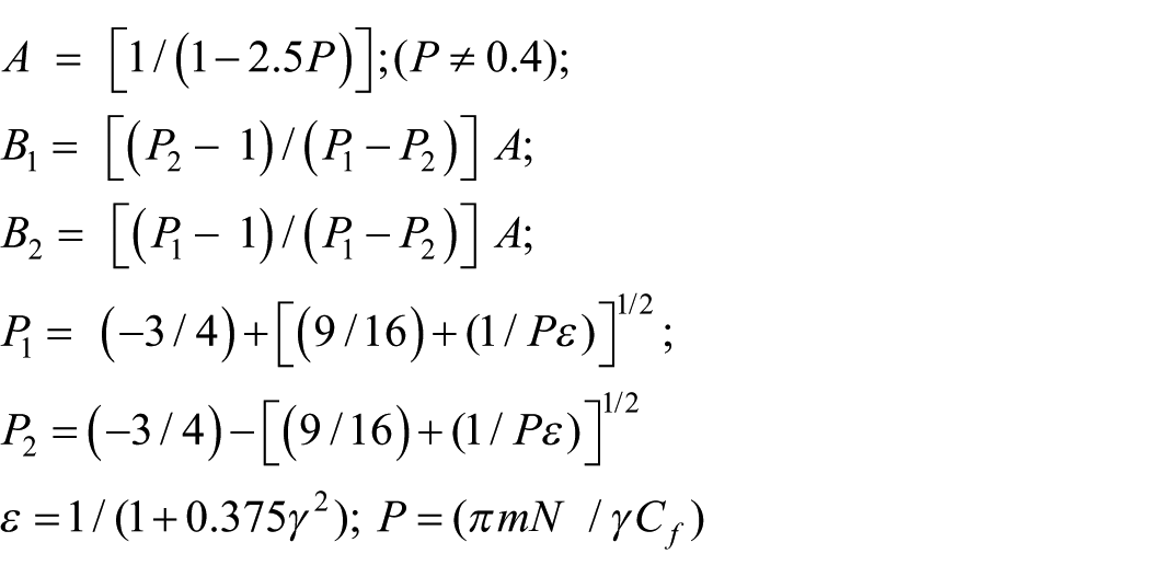
\begin{array}{l} A = [1 / (1 - 2.5 P)]; (P \neq 0.4); \\ B_{1} = [(P_{2} - 1) / (P_{1} - P_{2})] A; \\ B_{2} = [(P_{1} - 1) / (P_{1} - P_{2})] A; \\ P_{1} = (- 3 / 4) + {[(9 / 16) + (1 / P ε)]}^{1 / 2}; \\ P_{2} = (- 3 / 4) - {[(9 / 16) + (1 / P ε)]}^{1 / 2} \\ ε = 1 / (1 + 0.375 γ^{2}); P = (π m N / γ C_{f}) \end{array}

where γ is the wave breaking index (consider as H = 0.78d).

In the above equations, all the constants depend on the non-dimensional parameter P, which again depends on the lateral mixing parameter N that varies between 0 and 0.016. Komar (1977) has combined the above longshore current velocity distribution of Longuet-Higgins (1970) with Bagnold (1966) and formulated the distribution of sediment transport along the surf zone due to waves and longshore current as

I_{i} = K_{2} [C_{f} ρ V^{2} + 0.5 f ρ (0.25 γ^{2} g d)] V

(3)

where apart from the variables explained above, f is the coefficient for oscillatory wave motion, V is the local longshore current velocity, K₂ is the proportionality constant between available power and resulting sediment transport. This K₂ evaluated by integrating the above equation across the surf zone gives the equation as below

\begin{array}{l} I_{l} = K_{2} (\frac{1}{8} ρ γ^{2} f g) (\frac{A}{3} + \frac{B_{1}}{P_{1} + 2}) V_{0} X_{b}^{2} \tan α + \\ K_{2} C_{f} ρ (\frac{A^{3}}{4} + \frac{3 A^{2} B_{1}}{P_{1} + 3} + \frac{3 A B_{1}^{2}}{2 (P_{1} + 1} + \frac{B_{1}^{3}}{(3 P_{1} + 1)}) V_{0}^{3} X_{b} \end{array}

(4)

and this equation be equated to total transport rate given by Komar (1977) and solved for K₂.

$I_{l} = K P_{l s}$ (K = 0.77) gives rise to

\begin{array}{l} K P_{l s} = K_{2} (\frac{1}{8} ρ γ^{2} f g) (\frac{A}{3} + \frac{B_{1}}{P_{1} + 2}) V_{0} X_{b}^{2} \tan α + \\ K_{2} C_{f} ρ (\frac{A^{3}}{4} + \frac{3 A^{2} B_{1}}{P_{1} + 3} + \frac{3 A B_{1}^{2}}{2 (P_{1} + 1} + \frac{B_{1}^{3}}{(3 P_{1} + 1)}) V_{0}^{3} X_{b} \end{array}

(5)

Once K₂ is obtained, it will be substituted in equation (4) to get the sediment transport distribution along the surf zone.

Van Rijn (2007) proposed a simplified sediment load transport formula for bed load (q_b) and suspended load (q_s) as Both Van Rijn (a) and (b)

q_{b} = α_{b} ρ_{s} u d {(\frac{D_{50}}{d})}^{1.2} m_{f}^{1.5}

(6)

q_{s} = 0.015 ρ_{s} U D_{50} m_{f}^{2} {(D *)}^{- 0.6}

(7)

where $D * = D_{50} [(S - 1) g / υ^{2}]$ and D* is the dimensionless particle size, α_b = 0.015, d is the water depth (m), u is the depth averaged flow velocity (m/s), ρ_s is the specific density of sediment (kg/m³), D₅₀ is the median (measured as 0.48 mm) particle size (m), and m_f is the mobility factor. The mobility factor is found with the help of effective velocity and critical velocity due to waves and currents. The critical velocities due to currents depend on the sediment size and the instantaneous depth. The critical velocities due to waves depend on the wave period, sediment size, and specific density. Further details concerning the parameters are discussed by Van Rijn (2007).

Shallow water model

The current velocity due to tide (u and v) is obtained by solving the shallow water equation (SWE) (equation (8)), and it is used to find the tidal prism by empirical relations.

The mean flow equations governing for tide-induced current may be written in the form of SWEs. In a Cartesian horizontal coordinate system with the (x, y) axes lying over the mean sea level and the z-axis pointing upward, they can be written as

\begin{array}{l} \frac{\partial η}{\partial t} + \frac{\partial (u h)}{\partial x} + \frac{\partial (v h)}{\partial y} = 0 \\ \frac{\partial (u h)}{\partial t} + \frac{\partial (u^{2} h)}{\partial x} + \frac{\partial (u v h)}{\partial y} - (\frac{\partial (ε h u_{x})}{\partial x} + \frac{\partial (ε h u_{y})}{\partial y}) = \\ \frac{τ_{w x} - τ_{b x}}{ρ} g h \frac{\partial η}{\partial x} - d f v - \frac{1}{ρ} (\frac{\partial S_{x x}}{\partial x} + \frac{\partial S_{y y}}{\partial y}) \\ \frac{\partial (v h)}{\partial t} + \frac{\partial (u v h)}{\partial x} + \frac{\partial (v^{2} h)}{\partial y} - (\frac{\partial (ε h v_{x})}{\partial x} + \frac{\partial (ε h v_{y})}{\partial y}) = \\ \frac{τ_{w y} - τ_{b y}}{ρ} g h \frac{\partial η}{\partial y} + d f u - \frac{1}{ρ} (\frac{\partial S_{x x}}{\partial x} + \frac{\partial S_{y y}}{\partial y}) \end{array}}

(8)

where η is the free surface elevation, including wave setup and tide, u and v are the mean velocity vector components, h is the total depth (h = d+η) with d being the still water level. ε is the eddy viscosity, τ_wi the surface stresses, τ_bi is the bed friction stresses (i = x, y), and f is the Coriolis parameter. S_ij are the components of the radiation stress tensor that represent the excess momentum fluxes associated with the oscillatory wave motion. Appropriate water levels and wind velocities have to be specified for the simulation of tides. It has been observed that in long-wave simulation studies, the initial conditions do not affect the numerical solution. So it is usual in tidal simulation studies to assume the ocean to be initially at rest, before the introduction of the free surface perturbation or wind stress at the ocean surface.

The finite volume method (FVM) is chosen for the solving SWE as it will better conserve the mass and momentum in the truncated solution domain. To obtain a basic idea of the FVM, the reader is referred to the study of Roache (1998). And for a detailed description of the method, one should read the study of Ashford (1996). The FVM involves partitioning the domain into a set of non-overlapping control volumes. On each control volume, the integral form of the equations is required to hold. The solution unknowns are taken to be the cell-average quantities that interact through fluxes at the boundaries of the control volumes. Using the integral form of the equations guarantees that any discontinuities that arise in the solution will have the proper strengths (and speeds in an unsteady calculation). Several possible choices exist for the control volumes on an unstructured mesh. In this work, a cell vertex method is used in which the unknowns are associated with the mesh vertices, and the control volumes are taken to be the cells of the median dual mesh. The fluxes through the boundaries of the control volumes are computed using an upwind procedure based on Godunov’s (1959) method.

Results and discussions

General

The idea of the semi-numerical approach is to accommodate as much physics-based predictions as possible and minimize the presence of empirical uncertainties. Therefore, the computational time is very much minimized.

In this approach, breaker wave height, breaker angle are computed through spectral wave modeling. The spectral wave model requires least computational time and provides spectral wave properties. The distribution of wave height and direction for each month of a year is shown in Figure 5. In the above figures, the arrow represents the direction of the wave, and color legend indicates the wave height. It is observed that the nearshore wave transformations are clearly reproduced. Wave refraction, shoaling, and breaking occur in the nearshore. The wave breaker details based on the spectral approach are summarized in Table 2. The wave height ranges from 0.7 m in offshore to around 0.8 to 1 m at the breaking line.

Figure 5.

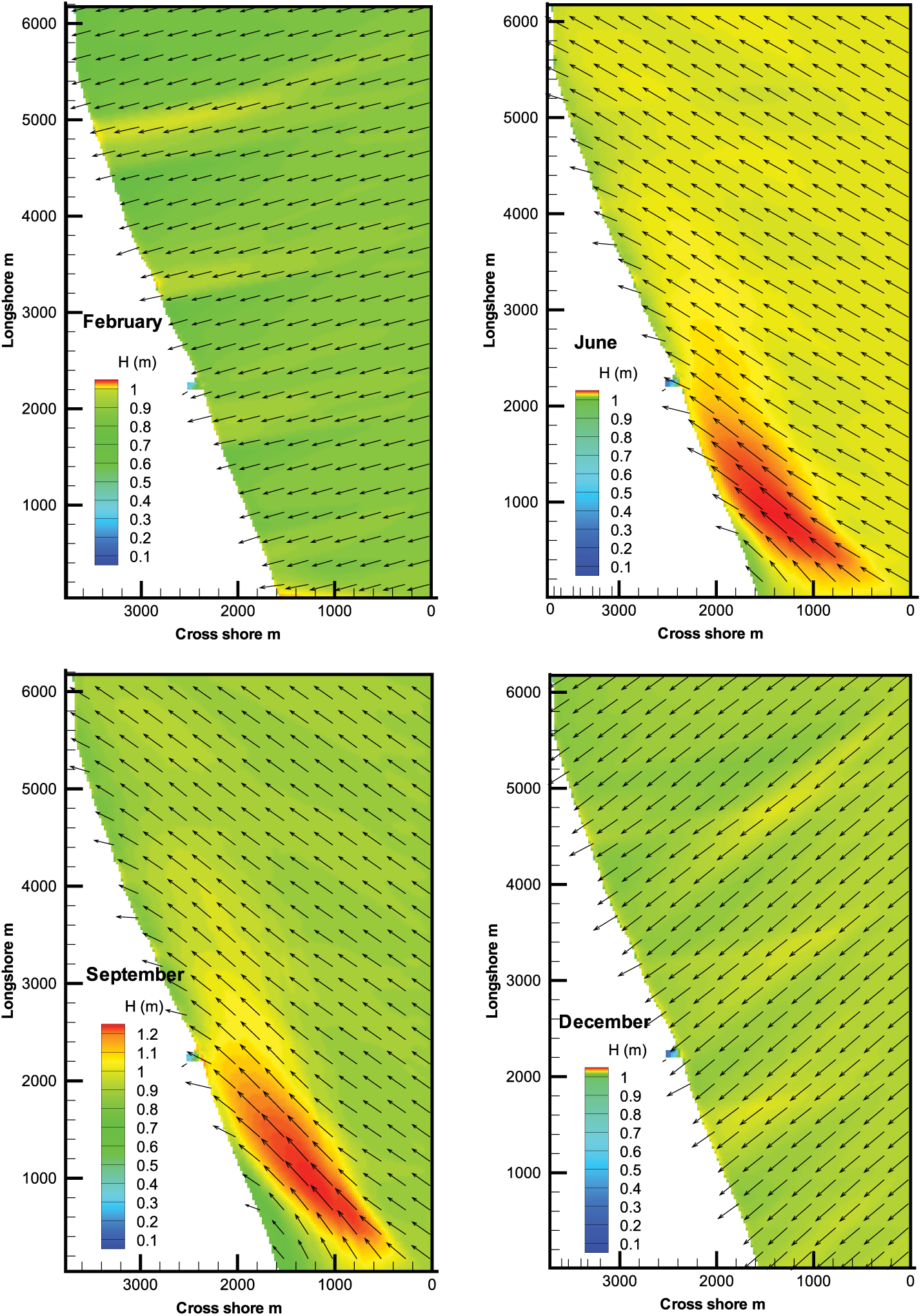
Typical wave height and direction for the month of February, June, September, and December

Table 2.

Breaking wave parameters and maximum longshore velocity from STWAVE.

Month	H_b (m)	α_b (°)	V_ls(max) (m/s)	x_b (m)
January	1.17	7	0.52	122
February	0.87	5	0.57	145
March	0.93	2	0.891	145
April	0.54	10	1.096	98
May	0.93	13	0.57	148
June	0.93	11	1.203	150
July	0.93	13	1.103	150
August	0.93	13	1.203	126
September	0.96	10	0.419	142
October	0.87	5	0.454	124
November	0.96	–8	0.490	132
December	0.96	–9	0.580	124

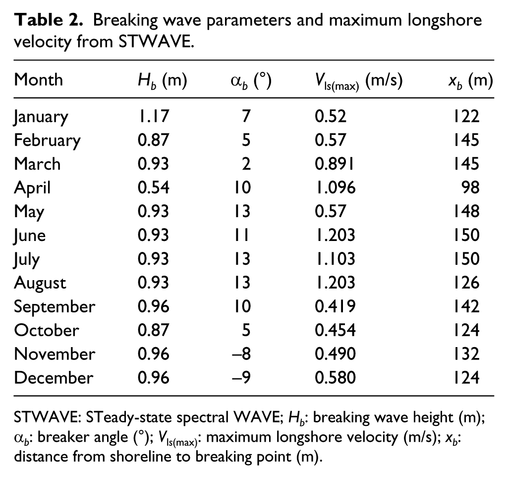
STWAVE: STeady-state spectral WAVE; H_b: breaking wave height (m); α_b: breaker angle (°); V_ls(max): maximum longshore velocity (m/s); x_b: distance from shoreline to breaking point (m).

Having computed breaking wave height and wave angle as above from the nearshore wave fields, the next step is to predict the longshore velocity. The maximum longshore velocity was computed using the relation by Longuet-Higgins (1970). The maximum longshore velocities range from 0.57 to 1.203 m/s.

The highest value of maximum longshore velocity (1.203 m/s) is observed during June and August during south west monsoon and 0.58 m/s for the month of December during north east monsoon. The maximum longshore velocity is less than 1 m/s during fair weather seasons. The average breaker line distance is about 145 m during south west monsoon and 125 m during north east monsoon. The longshore velocity distribution has been carried out by Komar (1977) distribution method across the surf zone. The longshore velocity distribution across the surf zone are projected in Figure 6, from which it is observed that the maximum longshore velocity occurs before the surf width (i.e. 150 m from the shoreline) and decreases gradually beyond the surf width, and at twice the length of surf width, it is found to be negligible.

Figure 6.

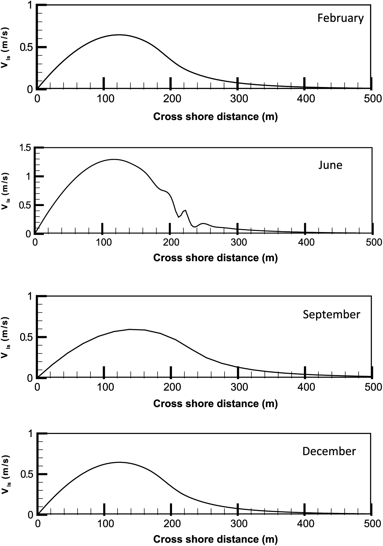
Distribution of longshore currents over the cross shore for the month of February, June, September, and December.

The longshore sediment transport rate is found by semi-numerical approach through sediment transport formula of Van Rijn (2007). Simultaneously using the breaker properties (Table 2), the longshore transport rate is obtained with the Coastal Engineering Research Center (CERC, 1984) method and that of the study of Kamphuis (1991). The longshore transport rates estimated through the above approaches are shown in Figure 7(a) to (c), while their inter-comparison is provided in Figure 7(d). The gross longshore transport rate estimated by semi-numerical approach is 0.11 Mm³/annum, and the total sediment transport rate is 0.09 Mm³/annum northerly and 0.02 Mm³/annum southerly. The gross longshore sediment rate computed by the application of Kamphuis (1991) is 0.09 Mm³/annum of which 0.08 Mm³/annum is northerly and 0.01 Mm³/annum southerly. The annual gross sediment transport rate estimated by CERC method is 0.18 Mm³. The sediment transport rate is estimated as 0.15 Mm³/annum northerly and 0.03 Mm³/annum southerly. Based on the results obtained, it is found that the sediment transport rate estimated by CERC gives higher value (Smith et al., 2003; Vijayakumar et al., 2014) and the study of Kamphuis (1991) gives lower value compared to that of the sediment transport rate estimated by Van Rijn (2007).

Figure 7.

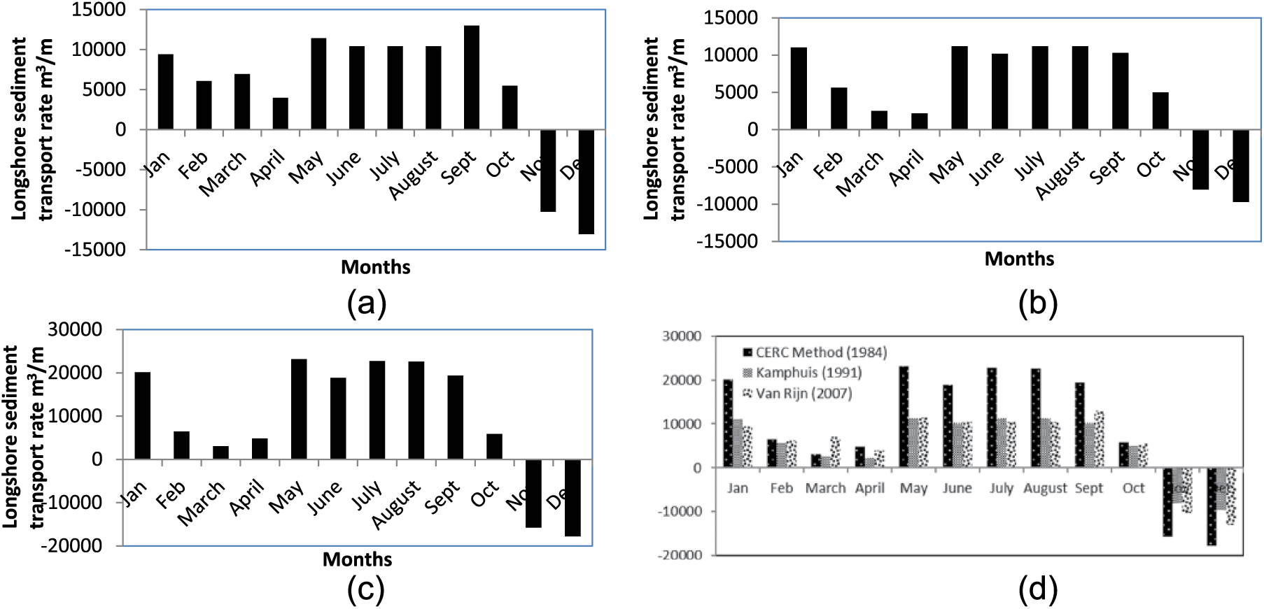
Monthwise longshore sediment transport rate: (a) study of Van Rijn (2007), (b) study of Kamphuis (1991), (c) CERC (1984) method, and (d) comparison of monthwise longshore sediment transport rate by semi-numerical approach.

Spring tidal prism

In tidally driven inlet dynamics, the estimation of tidal prism plays a key role. To estimate the tidal prism, the following parameters are essential. The tidal prism is estimated using the relation

P = \frac{T_{t i d e}}{π} U_{_{g o r g e}} A

(9)

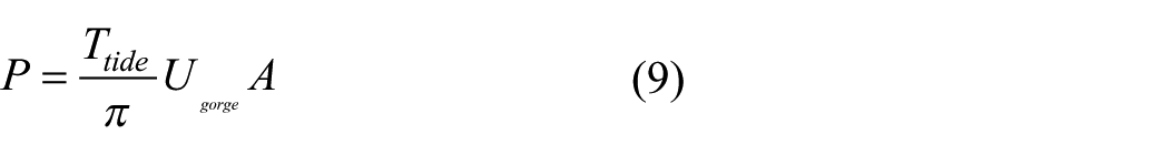
where P is the tidal prism (m³/cycle), T_tide is the tidal period for one cycle (s), U_gorge is the maximum velocity in the inlet gorge (m/s), A is the entrance cross section (m²) = (B_I*d_gorge), B_I is the inlet width (m), and d_gorge is the depth at the inlet gorge (m).

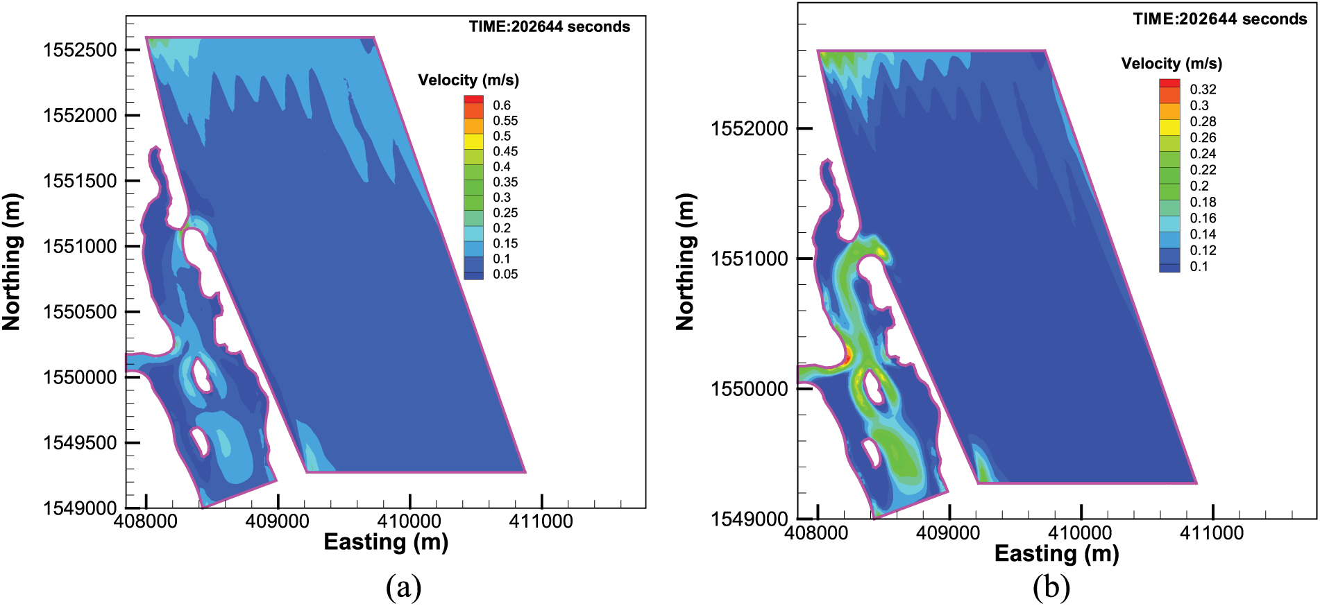
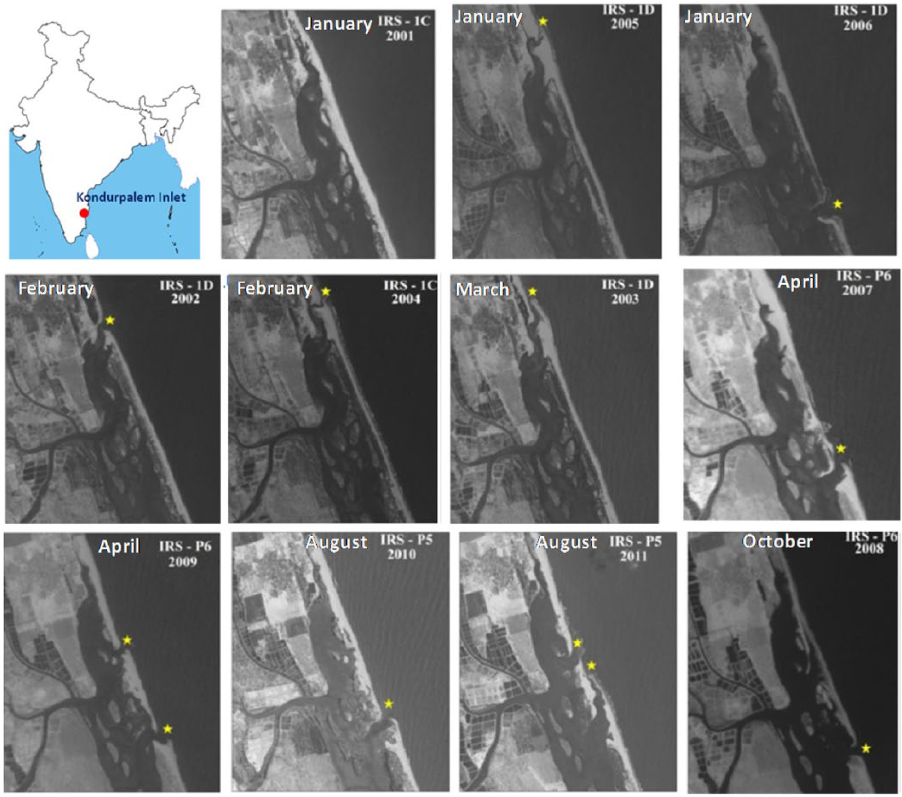
In the above relation, U_gorge is the maximum tidal velocity computed by solving the SWE. The domain considered for solving SWE and the velocity at inlet gorge is projected in Figure 8 for typical inlet widths. The area of the tidal entrance cross section is the product of the inlet width and depth at the inlet gorge. The depth at the inlet gorge is a measured data. The width of the inlet is observed from the satellite imageries collected. The satellite imageries of study area, from 2001 to 2011, are collected and analyzed. Based on the satellite imageries, the inlet and the shoreline of Kondurpalem area were mapped. The location map of the study area along with the variations of the mouth of Kondurpalem inlet over a decade from 2001 to 2011 are brought out in Figure 9. From the satellite imageries, it is generally expected that inlet opening will close during the monsoon and open during the non-monsoon season due to lack of longshore sediment transport. In the Kondurpalem inlet, a fine balance need to be maintained between longshore transport and tidal prism, due to which the effect of monsoon activity is felt in the months immediately after the monsoon. In order to explain this effect, the width of the inlet opening for different months is provided in Table 3.

Figure 8.

Velocity at the inlet gorge when the width is: (a) 20 m and (b) 150 m.

Figure 9.

Key map of Kondurpalem inlet and chronological location of openings.

Table 3.

Estimation of inlet width from satellite imageries from 2001 to 2011.

Month	No. of images considered	Inlet width (m)
January	4	0
February	8	20
March	4	115
April	4	150
May	6	120
June	16	100
July	4	70
August	4	50
September	4	30
October	4	20
November	4	75
December	4	60

Stability of inlets

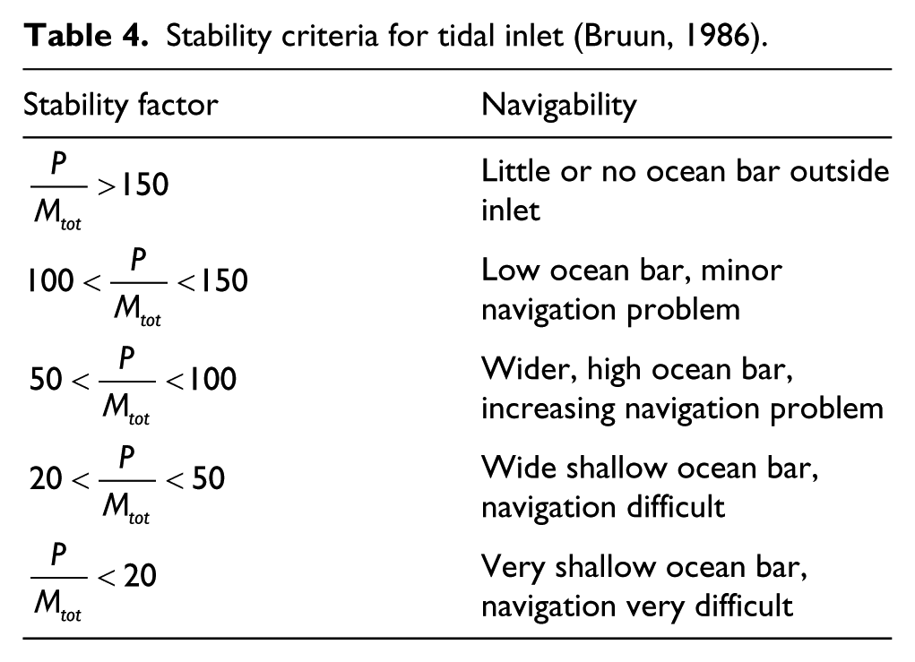
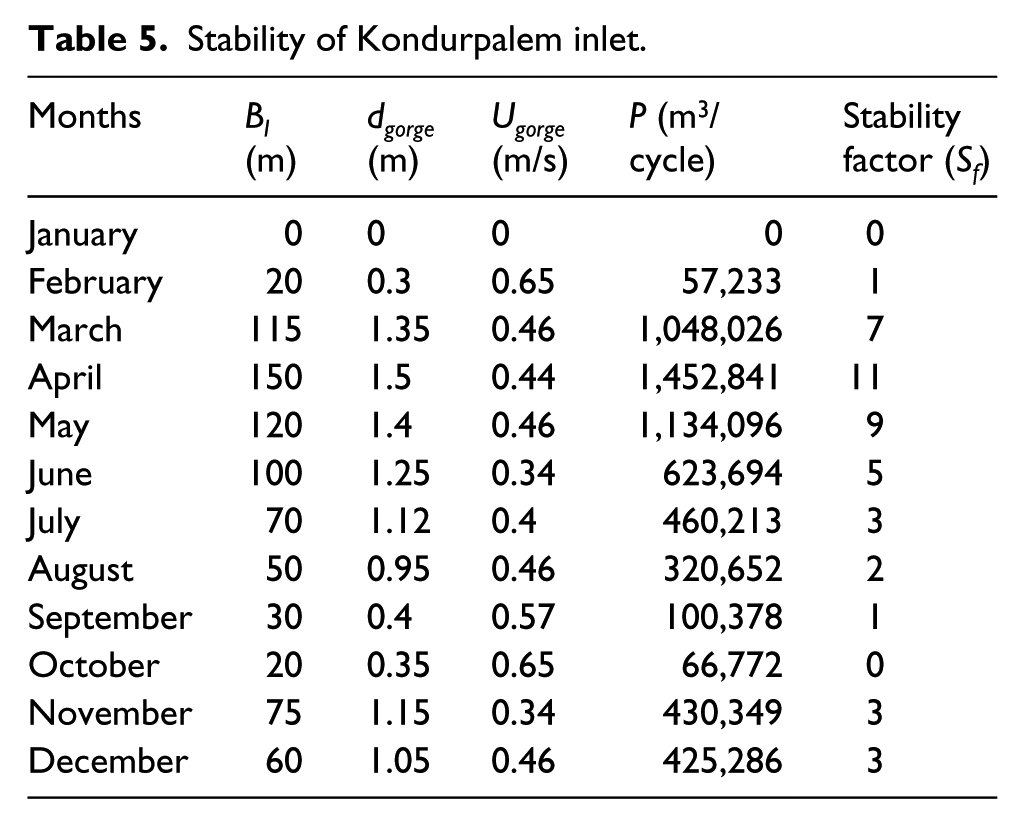
The criteria developed by Bruun (1986) based on the ratio of the tidal prism volume to the annual gross volume of sediment transport is shown in Table 4.The stability of the inlet is initially assessed with the existing condition (without training works) using the approach of Bruun (1986). The stability number for the inlet found using annual gross longshore sediment transport rate and spring tidal prism is shown in Table 5. It is observed that the stability number is less than 20 for all the months.

Table 4.

Stability criteria for tidal inlet (Bruun, 1986).

Stability factor	Navigability
$\frac{P}{M_{t o t}} > 150$	Little or no ocean bar outside inlet
$100 < \frac{P}{M_{t o t}} < 150$	Low ocean bar, minor navigation problem
$50 < \frac{P}{M_{t o t}} < 100$	Wider, high ocean bar, increasing navigation problem
$20 < \frac{P}{M_{t o t}} < 50$	Wide shallow ocean bar, navigation difficult
$\frac{P}{M_{t o t}} < 20$	Very shallow ocean bar, navigation very difficult

Table 5.

Stability of Kondurpalem inlet.

Months	B_I (m)	d_gorge (m)	U_gorge (m/s)	P (m³/cycle)	Stability factor (S_f)
January	0	0	0	0	0
February	20	0.3	0.65	57,233	1
March	115	1.35	0.46	1,048,026	7
April	150	1.5	0.44	1,452,841	11
May	120	1.4	0.46	1,134,096	9
June	100	1.25	0.34	623,694	5
July	70	1.12	0.4	460,213	3
August	50	0.95	0.46	320,652	2
September	30	0.4	0.57	100,378	1
October	20	0.35	0.65	66,772	0
November	75	1.15	0.34	430,349	3
December	60	1.05	0.46	425,286	3

It is also observed that the semi-numerical method over-predicts the stability number most of the time. The numerical approach provides a balanced estimation of the stability number. A comparison of these stability values with that of Brunn’s stability criterion as explained earlier suggests that the inlet would be unstable over all the months of the year. However, based on the satellite imageries and field observations, it is found that the inlet is open for a few months. Since Brunn’s criterion is a general requirement for major inlets, it may not be applicable to micro-tidal inlets. In order to bring out the mechanism of stability in case of micro-tidal inlets, the stability number was revisited. This is done by considering the dimension of a normal fishing boat (of length LOA = 7.5 m, beam B_b = 3 m, and draft D_b = 1.5 m). As per codal provisions (IS 4561), the width of the inlet should be 8B_b. Hence, the sufficient inlet width shall be 25 m. The depth in the inlet should be 1.2 times of the draft (d_gorge ~2 m). The lengths of the training walls are preferred to be about twice the surf width (~300 m). The revised stability criteria shall consider only these dimensions in the tidal prism. Hence, by considering the annual longshore drift and corresponding tidal prism with inlet dimensions as per navigational requirements, the stability number is found to be 5. This condition will not mean that the inlet will be stable, but will be open with some dredging requirement. This may be called as quasi-stable condition. However, to enable dredging and keep the opening constant, training works will be needed. The revised stability number for each month is presented in Table 6.

Table 6.

Stability of Kondurpalem inlet by considering the navigational requirements of small crafts.

Months	Navigational requirements of small crafts
Months	Spring tidal prism	Stability number	Navigability
January	0	0	No
February	381,554	3	No
March	1,552,632	10	Yes
April	1,937,121	13	Yes
May	1,620,138	11	Yes
June	997,911	7	Yes
July	821,809	5	Yes
August	675,057	5	Yes
September	501,890	3	No
October	381,554	3	No
November	748,433	5	Yes
December	810,069	5	Yes

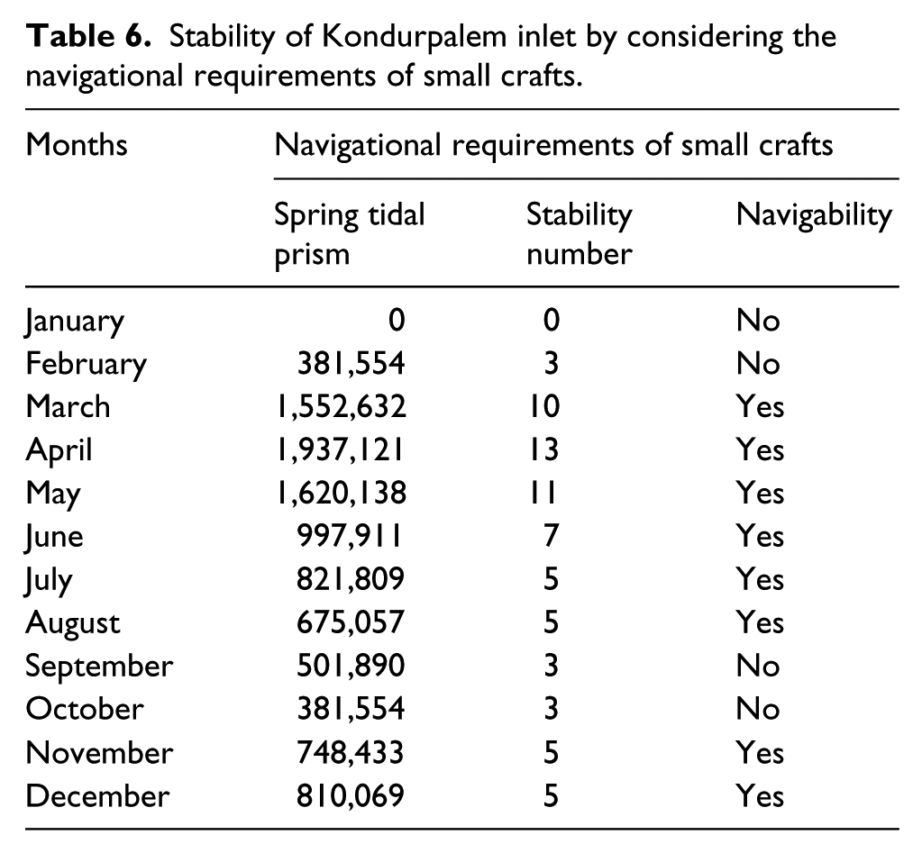
By considering the stability number to be 5, the inlet will be available for navigation except for the months of January, February, September, and October. This may be considered as the design basis for obtaining minimum opening dimension for providing training works. Observation from satellite imageries shows that except for the months of the January, February, and October, the inlet width is more than 25 m. During the months of January, February, and August to October, the depth at the inlet gorge has been observed to be less than 1 m as discussed earlier. Although the stability criteria satisfy the navigation, it is affected by the depth in the inlet. The observed depth in the inlet indicates the formation of shoals. Since, the inlet width is not uniform over the years, it is required to find the optimized width through training. The inlet would be marginally stable with a stability number 5 with some navigational difficulty. The inlet can be made navigable by dredging prior to monsoon.

Training and management of inlets

Based on the stability aspects as discussed in earlier section, the minimum width of the inlet and the depth at gorge must be maintained at 25 and 2 m, respectively. The lengths of the training walls are about 300 m (by considering the surf width and beach slope). By considering the above stated parameters of training walls and the wave climate and the breaking wave parameters, the shoreline evolution (Janardanan and Sundar, 1997) over a period of interval 1, 5, 10, and 25 years were carried out for the purpose of obtaining longshore sediment balance at the inlet. This balance quantity is that needs to be dredged. The balance thus obtained for different inlet widths of 50 and 75 m are shown pictorially in Figure 10.

Figure 10.

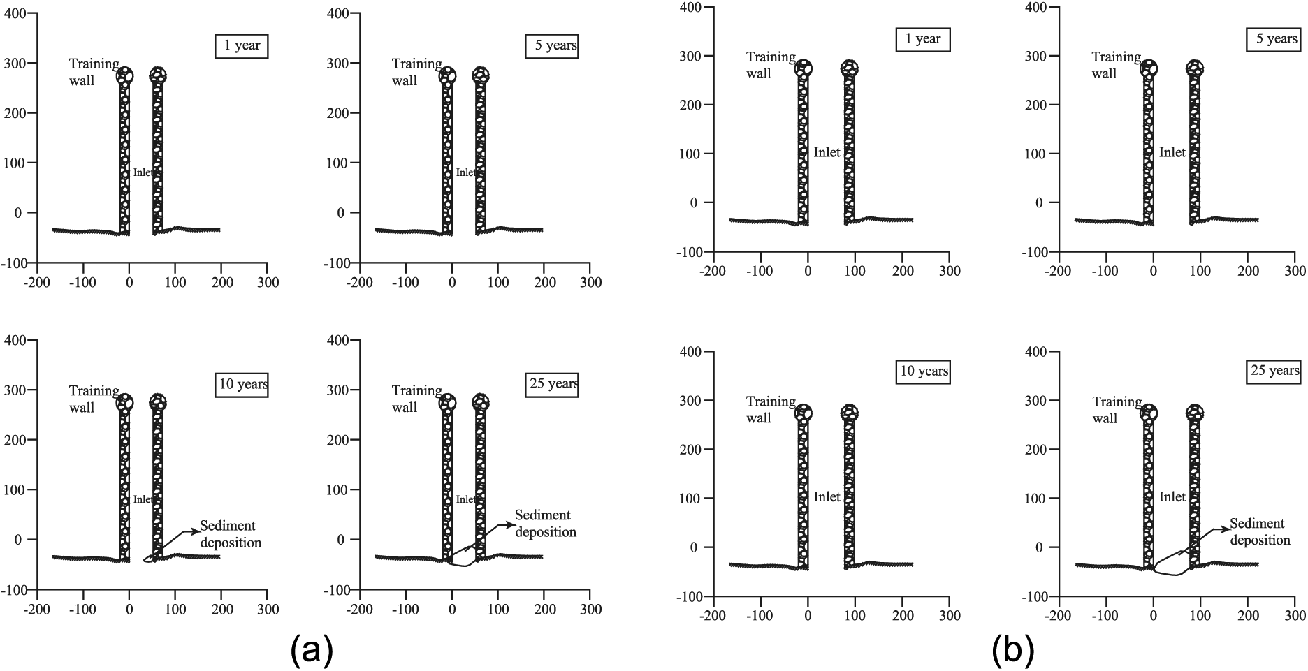
Siltation pattern near the mouth of the inlet in presence of 300-m-long training walls: (a) distance between the training walls = 50 m and (b) distance between the training walls = 75 m.

The results indicate the likely extent of shoal formation corresponding to the sediment balance at the inlet. The results for the 25-m inlet width show that there was no deposition at the end of first year. Over a period of 5 years, there was an accretion initiated in the inlet mouth, and it was not completely closed. At the end of 10 years, more accretion was observed in the mouth; and at the end of 25 years, the inlet is completely closed. The inlet width of 50 m shows that there is net accretion inside the inlet during the period of 10th year, and it increases further for the inlet width of 50 m, whereas for a width of 75 m, no accretion over the period of 10 years is noticed. For the inlet width of 100 m, a deposition during 10th year is noticed which tends to erode at the end of 25 years. However, the sediment deposition is more during 10th year compared to the inlet width lesser than 100 m. For the inlet width of 125 m, sediment accretion over the years starting from the initial stage is seen. The overall sediment balance of the inlet after the construction of training walls and aspect of the dredging for corresponding shoal removal is summarized in Table 7. As discussed earlier, the inlet of 50–75 m must be provided to maintain its mouth to be open all over the year. If the inlet width provided is 50 m, then the dredging cost for maintaining the depth of 2 m in the inlet is required at the end of 10 years. If the inlet width of 75 m is adopted, there is no need of dredging till the end of 10th year. With the minimum dredging or without any dredging, the inlet can be maintained without sand bar formation for a minimum duration of 10 years by providing the inlet width between 50 and 75 m and maintaining the depth at inlet gorge as 2 m.

Table 7.

Sediment balance over the years as predicted by shoreline evolution.

Inlet width	Area of shoal (m²)	1 year	5 years	10 years	25 years
25 m	Accretion (+ve)	0	286	599	1440
	Erosion (−ve)	102	087	199	478
	Net siltation	(−)102	(+)199	(+)400	(+)962
50 m	Accretion (+ve)	92	92	543	2285
	Erosion (−ve)	230	529	354	577
	Net siltation	(−)138	(−)437	(+)189	(+)1708
75 m	Accretion (+ve)	0	502	1004	5090
	Erosion (−ve)	502	1004	2008	2424
	Net siltation	(−)502	(−)502	(−)1004	(+)2666
100 m	Accretion (+ve)	568	1704	3408	5680
	Erosion (−ve)	1136	2272	1704	6248
	Net siltation	(−)568	(−)568	(+)1704	(−)568
125 m	Accretion (+ve)	2460	2766	6226	9987
	Erosion (−ve)	1845	1383	3113	2982
	Net siltation	(+)615	(+)1383	(+)3113	(+)7005

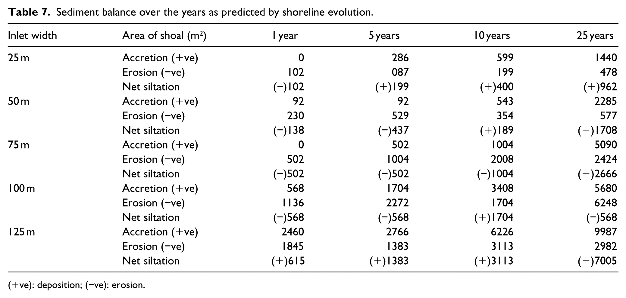
(+ve): deposition; (−ve): erosion.

Conclusion

Three different methods, namely, the study of Van Rijn (2007), the study of Kamphuis (1991), and CERC (1984) method, produced a longshore sediment transport rate bounded by the method of CERC (1984) on the higher side to an extent of about 50%, whereas the predictions through the method of Kamphuis (1991) is found to be less by an extent of about 57%.

In this work, a more practical approach for ascertaining stability for micro-tidal inlet is proposed. The approach that is taken by this work is to estimate the littoral transport rate and tidal prism and to then estimate the stability through the stability criteria of Bruun (1986). Usually, the computation involving morphodynamics need a lot more field data and is time-consuming. Hence, this step is avoided.

It is suggested that for the purpose of operating small fisherman and country boat through micro-tidal inlets, a stability number close to 5 may be considered suitable for micro-tidal inlets.

An approach is demonstrated to optimize the spacing between the training walls, considering sediment balance and dredging requirements. This analysis indicates that for Kondurpalem inlet, the spacing between the training walls is to be maintained as 50–75 m considering a gorge depth of 2 m.

Footnotes

Acknowledgements

The authors wish to thank National Institute of Ocean Technology (NIOT), Chennai, for providing assistance during the field data collection.

Declaration of conflicting interests

The author(s) declared no potential conflicts of interest with respect to the research, authorship, and/or publication of this article.

Funding

The author(s) received no financial support for the research, authorship, and/or publication of this article.

Author biographies

R Senthilkumar was a former research scholar in the Department of Ocean Engineering, Indian Institute of Technology Madras. His research interests includes Coastal engineering, Estuarine and Coastal Dynamics.

K Murali is a Professor in Department of Ocean Engineering, Indian Institute of Technology Madras. His research interest includes Coastal and Ocean Hydrodynamics, fluid structure interaction applied to Ocean Engineering and multi-phase flow simulations.

V Sundar is a Professor in Department of Ocean Engineering, Indian Institute of Technology Madras. His research interest includes Coastal and Ocean Hydrodynamics, Coastal and Shore protection structures. He was IAHR chairman for Asia Pacific division. He has been a visiting Professor for delivering lectures around the globe.

References

Ashford

(1996) An unstructured grid generation and adaptive solution technique for high Reynolds number compressible flows. PhD Thesis, The University of Michigan, Ann Arbor, MI.

Bagnold

(1966) An approach to the sediment transport problem from general physics. US government printing office.

Bruun

(1986) Morphological and navigational aspects of tidal inlets on littoral drift shores. Journal of Coastal Research 2: 123–145.

Chandramohan

Sanil Kumar

Nayak

(1991) Wave statistics around the Indian coast based on ship observed data, coast of India. Indian Journal Of Marine Science 20: 87–92

CERC (1984) Shore Protection Manual, vol. 1. Washington, DC: Superintendent of Documents, U.S. Government Printing Office.

Davies

(1964) What is a wave-dominated coast? Marine geology 60(1–4): 313–329.

Godunov

(1959) A difference method for numerical calculation of discontinuous solutions of the equations of hydrodynamics. Matematicheskii Sbornik 89(3): 271–306.

Hayes

(1979) Barrier Island Morphology as a Function of Wave and Tide Regime (ed Leatherman

). New York: Academic Press, pp. 1–29.

Janardanan

Sundar

(1997) Effect of uncertainties in wave characteristics on shoreline evolution. Journal of Coastal Research 13(1): 88–95.

10.

Kamphuis

(1991) Alongshore sediment transport rate. Journal of Waterway, Port, Coast and Ocean Engineering 117: 624–640.

11.

Komar

(1977) Beach sand transport: Distribution and total drift. Journal of the Waterway, Port, Coastal, and Ocean Division 103(2): 225–239.

12.

Kraus

(1998) Inlet cross-section area calculated by process-based model. In: Proceedings of the 26th conference on coastal engineering, Copenhagen, 22–26 June, pp. 3265–3278. Reston, VA: ASCE.

13.

Longuet-Higgins

(1970) Longshore currents generated by obliquely incident sea waves: 1. Journal of Geophysical Research 75(33): 6778–6789.

14.

Ranasinghe

Pattiaratchi

(1999) The seasonal closure of tidal inlets: Wilson inlet—A case study. Coastal Engineering 37: 37–56.

15.

Roache

(1998) Verification and Validation in Computational Science and Engineering, vol. 895. Albuquerque, NM: Hermosa Publishers.

16.

Smith

Wang

Zhang

(2003) Evaluation of the CERC formula using large-scale model data. In: Proceedings of coastal sediments, Geology faculty publications. Vol. 3. Paper 238. University of South Florida. Available at: http://scholarcommons.usf.edu/gly_facpub/238

17.

Suprijo

Mano

(2004) Dimensionless parameters to describe topographical equilibrium of coastal inlet. In: Proceedings of the 29th conference on coastal engineering, Lisbon, 19–24 September 2004, pp. 2531–2543. New York: ASCE.

18.

Thanh

Van de Kreeke

Stive

MJF

et al . (2012) Cross-sectional stability of tidal inlets: A comparison between numerical and empirical approaches. Coastal Engineering 60: 21–29.

19.

Van de Kreeke

(1998) Adaptation of the Frisian Inlet to a reduction in basin area with special reference to the cross-sectional area of the inlet channel. Physics of Estuaries and Coastal Seas. The Netherlands, Balkema, Rotterdam, pp. 355–362.

20.

Van de Kreeke

(2004) Equilibriumand cross-sectional stability of tidal inlets: application to the Frisian inlet before and after basin reduction. Coastal Engineering 51(5–6): 337–350.

21.

Van Rijn

(2007a) Unified view of sediment transport by currents and waves, I: Initiation of motion, bed roughness, and bed-load transport. Journal of Hydraulic Engineering 133(6): 649–667.

22.

Van Rijn

(2007b) Unified view of sediment transport by currents and waves, II: Suspended transport. Journal of Hydraulic Engineering 133(6): 668–689.

23.

Vijayakumar

Rajasekaran

Sundararajan

et al . (2014) Studies on the dynamic response of coastal sediments due to natural and manmade activities for the Puducherry coast. Journal of Marine Science 43: 1322–1326.

Stability of a micro-tidal inlet using semi-numerical approach

Abstract

Keywords

Introduction

Study area

Methodology

Komar Distribution method

Shallow water model

Results and discussions

General

Spring tidal prism

Stability of inlets

Training and management of inlets

Conclusion

Footnotes

Acknowledgements

Declaration of conflicting interests

Funding

Author biographies

References