Sage Journals: Discover world-class research

Abstract

Indian Space Research Organization had launched Oceansat-2 on 23 September 2009, and the scatterometer onboard was a space-borne sensor capable of providing ocean surface winds (both speed and direction) over the globe for a mission life of 5 years. The observations of ocean surface winds from such a space-borne sensor are the potential source of data covering the global oceans and useful for driving the state-of-the-art numerical models for simulating ocean state if assimilated/blended with weather prediction model products. In this study, an efficient interpolation technique of inverse distance and time is demonstrated using the Oceansat-2 wind measurements alone for a selected month of June 2010 to generate gridded outputs. As the data are available only along the satellite tracks and there are obvious data gaps due to various other reasons, Oceansat-2 winds were subjected to spatio-temporal interpolation, and 6-hour global wind fields for the global oceans were generated over 1 × 1 degree grid resolution. Such interpolated wind fields can be used to drive the state-of-the-art numerical models to predict/hindcast ocean-state so as to experiment and test the utility/performance of satellite measurements alone in the absence of blended fields. The technique can be tested for other satellites, which provide wind speed as well as direction data. However, the accuracy of input winds is obviously expected to have a perceptible influence on the predicted ocean-state parameters. Here, some attempts are also made to compare the interpolated Oceansat-2 winds with available buoy measurements and it was found that they are reasonably in good agreement with a correlation coefficient of R > 0.8 and mean deviation 1.04 m/s and 25° for wind speed and direction, respectively.

Keywords

Oceansat-2 winds spatio-temporal interpolation satellite winds inverse distance and time interpolation RAMA buoy

Introduction

Knowledge of surface wind fields over the sea is essential for a range of oceanographic, meteorological and climate investigations. Moreover, the surface wind field is a key variable in estimating the exchanges of momentum (kinetic energy) between the atmosphere and sea. It is fundamental to estimate fluxes of heat longwave radiation, moisture across the interface and for development, operationalization and validation of coupled ocean and atmosphere models. With the launch of satellites, the global ocean surface wind field is observable from space at near-mesoscale resolution. Measurement techniques using active microwave scatterometers have been developed, tested and being refined over the past three decades. Oceansat-2 was India’s second satellite built for the study of oceans as well as the interaction of oceans and the atmosphere to facilitate global and regional climatic studies (Jayaraman, 2007). Accurate observations of surface wind stress and wind velocity over global oceans are required for a wide range of meteorological and oceanographic studies (Ayina et al., 2006; Cotton, 2013). Winds are essential for nowcasting of weather and ocean/sea-state, as well as for improving weather forecasts via data assimilation in numerical weather prediction (NWP) models. It was dedicated to ocean research, as continuity of the operational services of Oceansat-1 with high application potentials. Oceansat-2 was launched from Satish Dhawan Space Centre, Sriharikota on 23 September 2009, using Polar Satellite Launch Vehicle (PSLV-C14) which had three payloads: (1) Ocean Colour Monitor (OCM), (2) Ku-band Pencil Beam Scatterometer (OSCAT) developed by Indian Space Research Organization (ISRO) and (3) Radio Occultation Sounder for Atmosphere (ROSA) developed by the Italian Space Agency. The mission goal of Oceansat-2 was to provide wind speed measurements of 4–24 m/s, with an accuracy of 2 m/s, and direction, with an accuracy of 20°. The scatterometer, a Ku-band pencil beam sensor similar to that onboard QuikSCAT satellite, provided surface wind vectors over global oceans with 2 days repeativity. Pencil beam scatterometer has the advantage of estimating wind direction at low wind speeds because of its viewing from four azimuth angles (Desai et al., 2000).

Measurements of surface winds over global oceans still continue to be sparse in space and time, thus causing hurdles for improvements in numerical predictions. Development of space-based technologies and geophysical retrieval techniques over the past decades has resulted in significant improvement in the observation frequency of surface winds over global oceans. The most prominent among these is the space-borne scatterometer (Chang et al., 2009). Space-based radiometers and altimeters are additional sources of ocean surface wind speed. Furthermore, synthetic aperture radar data have also been used to retrieve wind fields (Horstmann and Koch, 2005). Limitations and strengths of wind-measuring capability of each type of sensor and technique are briefly described by Sarkar (2003). For weather forecasting with NWP models to be reliable, it is necessary that the input data (such as ocean surface winds) be drawn from sources that are mutually consistent. Thomas et al., 2012 examined the consistency of oceanic winds measured by the new space-borne Oceansat-2 Scatterometer (OSCAT) with that measured by JASON Altimeter and buoy measurements. It was reported that the wind component standard deviations of OSCAT with respect to the European Centre for Medium-range Weather Forecasts (ECMWF) model winds and in situ buoy winds were better than 2.5 m/s (Stoffelen et al., 2010). Singh et al. (2012) investigated the quality of the OSCAT winds by comparing them with the global model surface winds from National Centers for Environmental Prediction (NCEP) analyses, Advanced Scatterometer (ASCAT) wind retrievals and buoy winds during July 2010. The three comparisons show that the root mean square (RMS) difference is in the range of 1.6–2.1 m/s. As the sea surface wind products from scatterometers flown onboard satellites are by-and-large acceptable and play an important role to create accurate NWP as well as the ocean-state predictions/analysis over the data sparse oceanic regions, the authors have attempted here to interpolate and validate the OSCAT wind products with respect to selected RAMA/TRITON/PIRATA buoy winds in order to assess whether the errors in OSCAT derived wind speed and direction are within the mission goal over the world ocean, so that the accuracy of interpolated OSCAT wind products can be further evaluated by driving the ocean models.

Data

In this study, the OSCAT ocean surface winds over the global oceans have been interpolated 6-hourly (and spatially over 1 × 1 degree resolution) using an efficient interpolation technique (inverse distance and time) and validated against few selected RAMA, PIRATA and TRITON buoys (six buoys) measurements for the month of June 2010. The details about the data used in this study are described under the following sub-headings.

Scatterometer data

ISRO reprocessed OSCAT Level-2B (L2B) wind data products (version 1.3, released in December 2011) were available for download through National Remote Sensing Centre (NRSC; www.nrsc.gov.in). These OSCAT wind vector products were generated based on the algorithms developed by Gohil et al. (2010). The scatterometer onboard OSCAT had provided these wind data with a high spatial resolution of 50 × 50 km with targeted accuracies of 10% (RMS) and 20° (RMS) for wind speed and wind direction, respectively. In this study, the MATLAB code developed by SAC (Maria Antonita and Kumar, 2010) was used to extract the said geophysical parameters, that is, wind speed and direction from Oceansat-2 scatterometer L2B HDF5 files. Figure 1 shows a sample OCEANSAT-2 wind data distribution along the satellite tracks for 1 day (repeativity 2 days). Since there were obvious data gaps (and missing data as well) and time gaps during the global coverage of OCEANSAT II, the gridded wind fields were prepared through spatio-temporal interpolation of these winds (Swain and Umesh, 2013) at 6-hour intervals over 1º × 1º resolution, and the details of which are presented under methodology. Figure 2 shows a sample OSCAT (observed/measured) contoured wind field before interpolation and Figure 3 also represents the OSCAT observed winds (contour plot) with large data gaps which becomes a challenge for a reliable interpolation.

Figure 1.

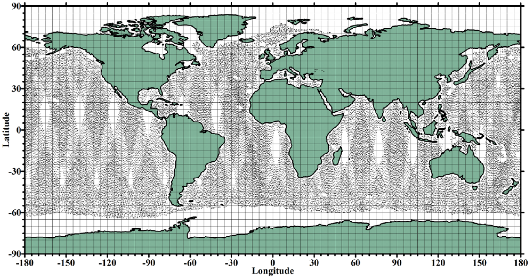
A sample OSCAT wind data distribution along the satellite tracks for one selected day, 09 June 2010 (Julian Day 158, 2010).

Figure 2.

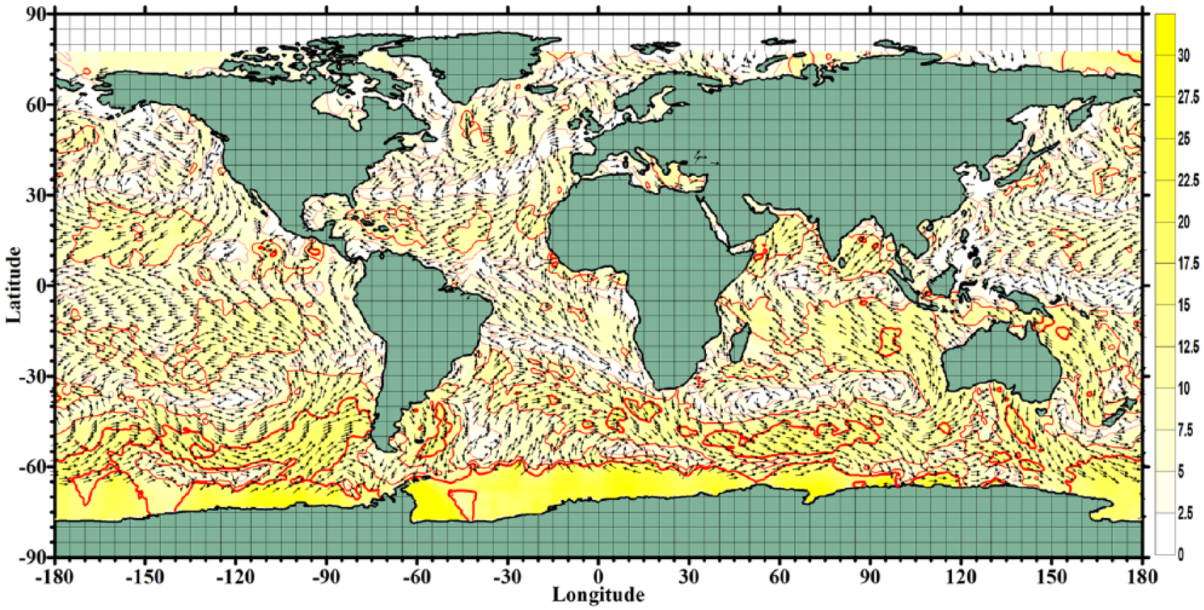
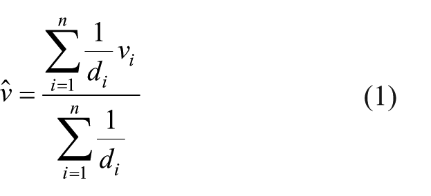
A sample of OSCAT observed winds (colour scale shows wind speed in m/s and direction with arrows) for 25 June 2010 (Julian Day 174).

Figure 3.

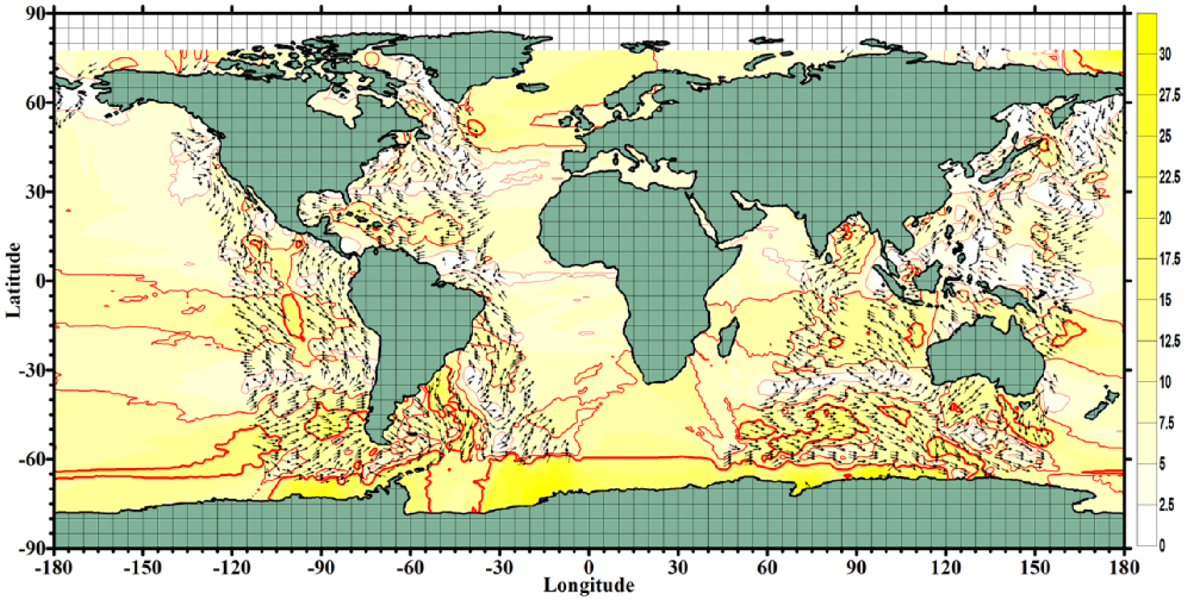
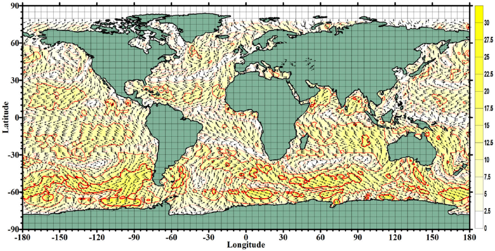
A sample of OSCAT observed winds (colour scale shows wind speed in m/s and direction with arrows) for 26 June 2010 (Julian Day 175) indicating large data gaps (missing data).

RAMA/PIRATA/TRITON buoy data

The Tropical Moored Array Programs (TMAP) consists of three different type of Tropical Atmosphere Ocean Buoy Arrays (TAOBA) such as Research Moored Array for African–Asian–Australian Monsoon Analysis and Prediction (RAMA; McPhaden et al., 2009) in the Indian Ocean, Prediction and Research Moored Array (PIRATA; Bourles et al., 2008) in the Atlantic and Tropical Atmosphere Ocean/Triangle Trans-Ocean Buoy Network (TAO/TRITON; Kuroda and Amitani, 2000; McPhaden et al., 1998) in the tropical Pacific. Since from their implementations, the high-quality time series data from the moored arrays have improved the understanding and prediction of climate variability and climate change (McPhaden et al., 2009). The scatterometer wind verification generally relay on the comparison between wind models and the sensor data or on the inter-comparison with meteorological buoy data (Chakraborty et al., 2013; Vogelzang et al., 2011). The measurements on the RAMA surface floats include the meteorological parameters like air temperature, relative humidity and wind velocity at a height of 3–4 m above the mean sea level (MSL). Daily averages of all data and several hourly samples per day of most meteorological variables are transmitted to shore in real time via Service Argos. These data placed on the GTS are used in operational weather, climate and ocean forecasting.

The locations of six selected buoys (RAMA, PIRATA and TRITON) for validations (McPhaden et al., 2009) with OSCAT data are shown in Figure 4. Basically with the use of the above buoy winds, an attempt has been made to compare OSCAT-interpolated winds (speed and direction, buoy winds corrected to 10 m level) for an assessment on the quality of gridded winds which can be used as model inputs for ocean-state hindcasting. As indicated above, the interpolated sea surface winds (at 10 m) from OSCAT over the globe will be evaluated against the said RAMA, PIRATA and TRITON buoys data for the period 01–30 June 2010. These buoy observations on winds were downloaded from the website www.pmel.noaa.gov for the Indian, Atlantic and Pacific Oceans (10-minute averages). The simplest method proposed by Hsu et al. (1994) and used operationally by NDBC (National Data Buoy Center) was adopted for conversion of buoy winds to 10 m. The accuracies of these buoy wind speed and direction are 0.3 m/s and 20°, respectively (McPhaden et al., 1998). Further details and particulars of the buoy sensors are given by McPhaden et al. (1998, 2009).

Figure 4.

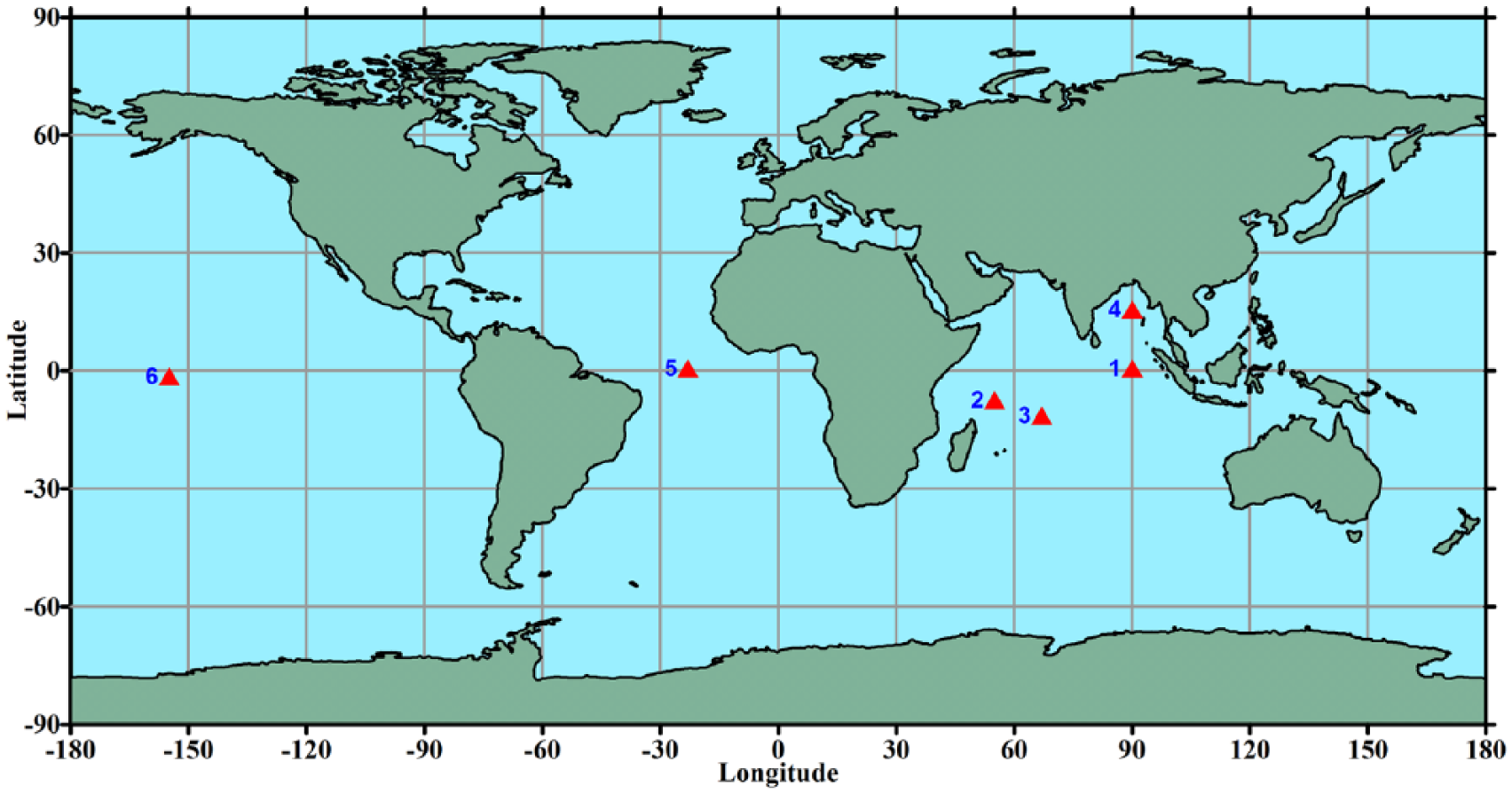
RAMA (labelled 1, 2, 3 and 4), PIRATA (labelled 5) and TRITON (labelled 6) buoy locations.

Methodology

The daily OSCAT winds were available with complete information on location and time of observations (in between 0000 hour to 2400 hours). The requirement of spatio-temporal interpolation of OSCAT data (U₁₀, at 10 m above the sea surface) to derive 6-hour wind fields was absolutely necessary for an evaluation and optimal utilization of space-borne wind measurements, as the satellite can only measure winds along its swath (repeativity 2 days). Second, there are obviously data gaps as shown in Figures 1 and 3 (between the tracks and missing data). In addition, the quality of data is also not satisfactory near to land/coast line. Considering these facts, the simplest but most efficient procedure of inverse time and distance interpolation was adopted in this article and it was found to be suitable with a space and time window of 1.5° and 1 day respectively over the spherical earth, which is explained below.

Before we discuss about inverse time and distance interpolation, we examined the cases where there are large data gaps as shown in Figure 3. The proposed interpolation cannot achieve expected results in such cases. Hence, to fill up the large data gaps beyond one degree, Laplacian smoothing (IMSL 1987) was applied iteratively if the measured data are not available all around the selected grid points for interpolation (Figure 3). The wind is described as having both a direction and a magnitude (speed), and it is therefore a vector quantity. Although the wind is a vector quantity, the wind direction and speed can be treated separately as scalar values. In collecting wind data, samples are typically collected at a high frequency and then averaged over a time period of a few minutes to an hour. Depending on the application in vector averaging, the orthogonal components of the wind are measured and then they are used to derive the orthogonal components. To obtain the vector-averaged speed and direction, the components are summed and vector averaged at the end of the averaging time. As we know wind is a vector quantity, the zonal and meridional components of wind, u and v were estimated and the resultant u and v components were used to estimate back the U₁₀ and its direction. Laplacian smoothing is one of the most commonly used mesh smoothing algorithms for a uniformly spaced two-dimensional array and by far the most popular smoothing method due to its simplicity and time efficiency (Vartziotis and Himpel, 2014). The basic idea behind Laplacian smoothing is simple and computationally straightforward. Mesh smoothing is the process of changing vortex positions in a mesh in order to improve the mesh quality for finite element analysis. Despite its long history, the original Laplacian has been presented as a heuristic method almost everywhere in engineering literatures (Freitag, 1997). However, Laplacian smoothing can be derived from a finite approximation of the Laplace operator. In particular, it efficiently minimizes a certain convex mesh quality function with a guaranteed and unique result. In the past, the efficient methods used for interpolating sparse data measurements onto a regular mesh are weighted interpolation, least-square polynomial interpolation and optimum interpolation (William et al., 1979). In this study, all the qualified OSCAT measurements (excluding the spurious values) available within each 1° grid were considered and vector-averaged without considering the time of satellite passage at this stage. The grids which had less than two data points or no data were filled by smoothing the wind vectors several times, by repeating the operation until the values do not vary/improve beyond 2.0%. The grid points pertaining to the land area were appropriately flagged for exempting the operation. It may be noted that the grid averages as well as the data gaps filled (1° × 1° resolution) by smoothing were finally time stamped as per the passage of OSCAT which coincides with the centre of the grid. After filling such large data gaps, the proposed inverse time and distance interpolation were applied to estimate winds every 6 hours as per the procedure described below.

The following most familiar equation of inverse distance and time interpolation was adopted to interpolate u and v with a space and time window as indicated above

\hat{v} = \frac{\sum_{i = 1}^{n} \frac{1}{d_{i}} v_{i}}{\sum_{i = 1}^{n} \frac{1}{d_{i}}}

(1)

where $\hat{v}$ is the value to be estimated (both for u or v components), v_i = i^th known value and d_i, …, d_n is the distances (km) or time of separations (duration in hours) for the n data points from the centre point whose value is being estimated. Naturally, the spatial interpolation (distance) was followed by temporal (time) interpolation (6 hours) as the second step. During every step of spatio-temporal interpolation, the original OSCAT measurements were retained or remained unchanged if there were more than two measurements; and the stamped time is within 3 hours on either side of 6-hour gridded fields (0000, 0600, 1200, 1800 and 2400 hours).

The inverse distance or time weighting is the most common interpolation method using equation (1). Basically, a neighbourhood about the interpolated point was identified and a weighted average was calculated for the observation values within its neighbourhood. The weights are a decreasing function of distance/time. This procedure allows very fast calculations by allowing the influence of distance/time being the integral part of the estimation as the measured values closest to the prediction location/time is considered to have more influence on the predicted value (here wind) than those farther away. Through trial and error, it was decided to consider a total of nine data points (n, equation (1)) for the spatial interpolation within a search radius of 1.5° to fill the data gaps for each day without disturbing the original measurements. Subsequent to the spatial interpolation, temporal interpolations were carried out considering 1 day time window for temporal interpolation of winds every 6 hours and by retaining the original OSCAT observed estimates as stated.

Results and discussion

The OSCAT winds for the month of June 2010 were subjected to spatio-temporal interpolation as per the method described above and 6-hour global wind fields (0°E to 360°E and 78°S to 78°N) were generated over 1° × 1° resolution. Figures 5 and 6 represent the two-sample interpolated winds for 1200 hours of 25 June 2010 and 1200 hours of 26 June 2010, respectively. If we compare the OSCAT measured winds of 25 and 26 June 2010 (contour plots as shown in Figures 2 and 3) with the interpolated winds as shown in Figures 5 and 6 following the present technique of inverse distance and time presented in this study, the results appear highly encouraging. It may be noted that the measured data as shown in Figures 2 and 3 were observed by OSCAT covering the whole day (0000–2400 hours), while Figures 5 and 6 represent the interpolated winds for a particular instant of time, that is, 1200 hours on 25 and 26 June 2010, respectively. It is also seen from the southernmost band (region of ice coverage) where there is no OSCAT data, and the interpolated winds reveal quite realistic representation of the nearest neighbourhood. The same is the case with the rest of the regions where data are either not available (very large gaps) or regions of gaps between the two adjacent swaths. One may surely appreciate the interpolated data much more if we compare specially the regions of large data gaps as shown in Figures 3 and 6. Therefore, the authors suggest that such interpolated wind fields can be used to drive the state-of-the-art numerical models to predict ocean-state so as to experiment and test the utility/performance of satellite measurements alone in the absence of blended fields. The technique can be easily adopted for other satellites which provide wind speed as well as direction data. However, the accuracy of input winds is obviously expected to have a perceptible influence on the predicted ocean-state parameters.

Figure 5.

OSCAT-interpolated winds (speed in m/s and direction with arrows), 25 June 2010 (1200 hours).

Figure 6.

OSCAT-interpolated winds (speed in m/s and direction with arrows), 26 June 2010 (1200 hours).

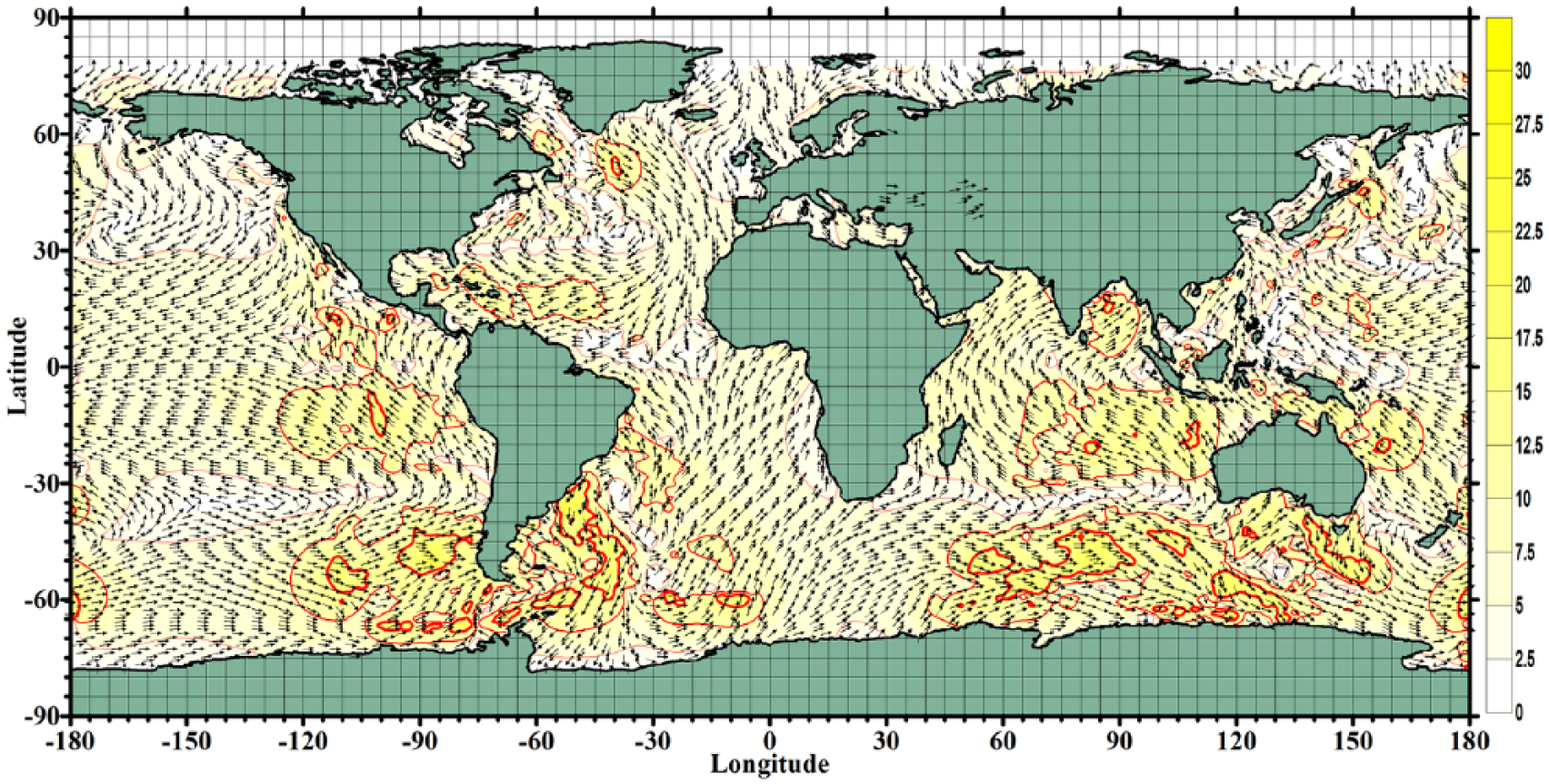
To test the utility and performance of sea-state prediction using satellite measurements alone (in the absence of blended fields), the wave models WAM Cycle 4.5.3 (The WAMDI Group, 1988) and WAVEWATCH-III (Tolman, 2009) were executed using these 6-hour interpolated OSCAT winds over the globe for the month of June 2010. The global grid system of the wave models (Umesh et al., 2013) covered the geographical extent, 0° to 360°E and 77°S to 77°N as shown in Figure 7 with a resolution of 1° × 1°. The bathymetric map had been constructed from ETOPO2 data. WAM used 25 frequencies ranging from 0.04177 Hz to 0.41145 Hz and 12 directions (constant increment), whereas WAVEWATCH-III also used 25 frequencies ranging from 0.0412 to 0.4056 Hz and 24 directions with constant increment. The sample model outputs of significant wave height (m) and mean wave direction are shown with arrows for 25 June 2010 (1200 hours; Figure 7). The spatial variability of these output parameters revealed very good representation of the prevailed wind over the global oceans. Moreover, both the model outputs also compare well with each other. However, it may be kept in the mind that the accuracy of interpolated/input ocean surface winds is expected to have a perceptible influence on the predicted sea-state parameters, which can be further quantified by validating with measured wave variability, which is not within the scope of this article.

Figure 7.

Sample outputs of wave model hindcasts of (a) WAM and (b) WAVEWATCH-III for 25 June 2010, (1200 hours) using interpolated OSCAT winds. Contours show significant wave height in metres and mean wave direction shown with arrows.

As indicated earlier, some attempts are also taken in this study to compare the interpolated OSCAT winds with available buoy measurements. Numerous studies have been reported earlier on the comparison of scatterometer wind observations from different space-borne platforms over the Indian Ocean with moored buoys and research vessels (Bentamy et al., 2002; Dickinson et al., 2001; Ebuchi et al., 2002; Goswami and Rajagopal, 2003; Goswami and Sengupta, 2003; Satheesan et al., 2007). The OSCAT wind verification was reported by researchers (Chakraborty et al., 2013; Jayaram et al., 2014; Portabella and Stoffelen, 2009; Singh et al., 2012; Stoffelen and Verhoef, 2011; Stoffelen et al., 2010; Thomas et al., 2012; Udaya Bhaskar et al., 2016; Vogelzang et al., 2011). Goswami and Sengupta (2003) carried out a comparison of QuikSCAT with two buoys in the Indian Ocean, and the Root Mean Square Vector Difference (RMSVD) was observed to be 1.4 m/s for both zonal and meridional components. Goswami and Rajagopal (2003) showed the impact of scatterometer data assimilation in numerical models to improve the weather forecast over India. Satheesan et al. (2007) had evaluated the performance of QuikSCAT wind vectors against in situ buoy observations over the Indian Ocean and reported the mean difference in wind speed and wind direction as 0.37 m/s and 5.8° and the RMS deviations as 1.57 m/s and 44.1° averaged over a period of 2000–2003. Sudha and Prasada Rao (2013) compared the OSCAT winds against RAMA buoy (considered 8 buoys) winds over the Indian Ocean and Triangle Trans-Ocean Buoy Network (TRITON) over the Pacific Ocean and reported that the OSCAT wind speed errors are within the mission goal, but the wind direction errors are higher and the OSCAT wind speeds are relatively more accurate over the Indian Ocean.

Studies were also carried out using daily and 12-hour gridded analysed wind vectors (AWVs) over global ocean (Chakraborty and Raj Kumar, 2013) which were generated using the simple spatial interpolation scheme of ‘box averaging’, with a horizontal resolution of 0.5° × 0.5°. For daily analysed winds, observations only from Oceansat-2 Scatterometer (OSCAT) were used. The 12-hour AWVs were generated by combining the data from both OSCAT and ASCAT. The daily and 12-hour analysed winds were validated using in situ observations from 97 global moored buoys and data from European Centre for Medium Range Weather Forecasting analyses for a period of 9 months. The validation result (Chakraborty and Raj Kumar, 2013) showed good agreement between AWV products and the buoy and model analysis data, yielding a standard deviation of around 2 m/s in wind speed and around 20° in wind direction. Wind measurements (Chelton and Michael, 2005) by the National Aeronautics and Space Administration (NASA) scatterometer (NSCAT) and the SeaWinds scatterometer on the NASA QuikSCAT satellite were compared with buoy observations to establish that the accuracies of both scatterometers are essentially the same. The scatterometer measurement errors are best characterized in terms of random component errors, which are about 0.75 and 1.5 m/s for the along-wind and cross-wind components, respectively. Wind products from QuikSCAT against JASON and 1 year (2010) of OSCAT data against JASON were compared (Thomas et al., 2012) to study the inter-consistency of ocean surface wind speeds, and it revealed that the bias and standard deviation between JASON and QuikSCAT (OSCAT) over the entire range of wind speeds is −0.29 (–0.31) m/s and 1.48 (1.55) m/s, respectively. The correlation coefficient for both QuikSCAT and OSCAT with respect to JASON over the entire 0–25 m/s range was found to be 0.92. The estimated mean percentage error for OSCAT wind speed and direction were 12.5% and 8.0%, respectively, when compared with RAMA buoy measurements (Siddharth and Nandu, 2013). These studies implied that as far as wind speed is concerned, OSCAT observations can be used to fill the gaps when there is non-availability of QuikSCAT from 2010 onwards for various applications. However, in this study, specifically for the validation purpose, OSCAT-interpolated wind vectors were collocated with the earlier mentioned buoy winds (RAMA, PIRATA and TRITON) both in space and time. The nearest four grids were selected and the data were interpolated following the same inverse time and distance approach attempted in this study to estimate wind speed and direction (OSCAT). Similarly, the nearest interpolated/estimated values which correspond to the past and future time zones have been interpolated (temporal) linearly to estimate 6-hour winds. The OSCAT and buoy data plots for the comparisons are shown in Figures 8 to 10 in the following.

Figure 8.

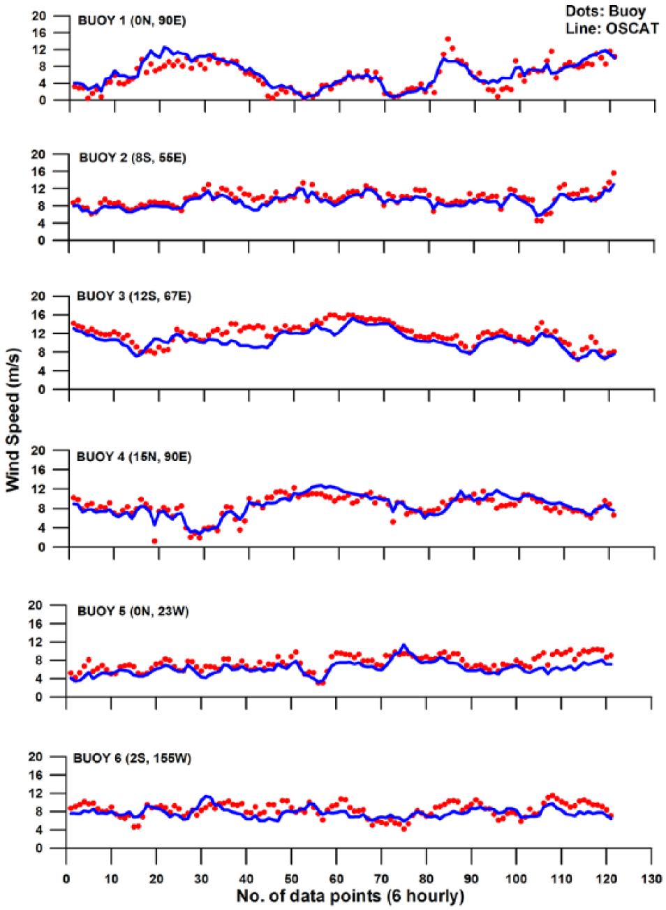
Comparison of 6-hourly buoy (RAMA, PIRATA and TRITON) and OSCAT wind speed at six selected locations for 01–30 June 2010.

Figure 9.

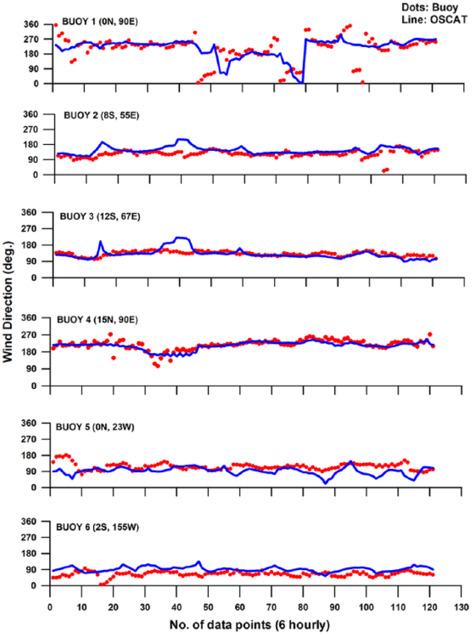
Comparison of 6-hourly buoy (RAMA, PIRATA and TRITON) and OSCAT wind directions at six selected locations for 01–30 June 2010.

Figure 10.

Combined scatter plots for 6 hourly observed (in situ buoy measurements): (a) OSCAT wind speed and (b) direction (01–30 June 2010) considering all the six buoy data shown in Figures 8 and 9.

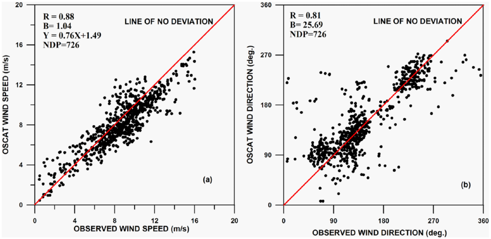
The wind speed comparisons between OSCAT (continuous line) and buoy winds (red solid circles) at 6-hour intervals for six selected buoy locations as shown in Figure 8 revealed a reasonable correlation (coefficient of correlation R = 0.88) and mean deviation of 1.04 m/s (B) for the wind speed range of 1–16 m/s as shown in the scatter plot (Figure 10, Number of Data Points (NDP) = 726). In the scatter plot, the line of no deviation is shown to have an assessment of the comparison/departure between the OSCAT winds and buoy observations. Further to the line of no deviation, the equation of the linear fit (Y = BX + A) as per its convention is also shown for indicating the constant of departure (A) and slope (B) between the independent (X) and independent (Y) variables. Similarly, as shown in Figure 9, the comparison of wind directions between OSCAT and buoys also revealed correlation coefficient of more or less similar magnitude (R = 0.81) with a mean deviation (B) of 25.0°. By and large, the comparisons were quite encouraging. It may be noted that the present comparison is well in agreement with the earlier studies exhaustively described/reviewed in the above paragraph and it is better compared to some of the earlier results.

Conclusion

In this article, the OSCAT winds over the global oceans have been interpolated 6 hourly using the most common interpolation technique (inverse distance and time) and the performance of the technique has been studied for the selected month of June 2010. The authors have implemented the said interpolation scheme, as the OSCAT measurements are available only along the OSCAT tracks (repeativity 2 days) and there were small as well as large data gaps in measurements (geophysical products). The following conclusions were drawn from this study:

The study revealed that the present spatio-temporal interpolation scheme and the 6-hourly global wind fields generated over 1° × 1° degree grid resolution can be utilized for sea-state prediction and the performance can be evaluated using in situ data.

The utility of the interpolated winds and the performance of two latest third-generation models such as WAM and WAVEWATCH-III are also demonstrated which could reveal very good representation of the model outputs versus the prevailed winds over the global oceans.

Furthermore, the interpolated winds obtained from OSCAT measurements were compared with in situ buoy observations such as RAMA, PIRATA and TRITON over the Indian, Pacific and Atlantic Oceans, respectively, during June 2010. The comparison of OSCAT-interpolated wind speed at 6-hour intervals for the six selected buoy locations revealed considerable agreement with a correlation coefficient of 0.88 and mean deviation of 1.04 m/s. Similarly, the comparison of wind directions (OSCAT and buoys) also revealed a correlation coefficient of 0.81 and a mean deviation of 25.0°.

Footnotes

Acknowledgements

The authors express their sincere thanks to Director, NPOL and Group Head, Ocean Sciences for their encouragement and support provided to carry out this work. This is a part of the collaborative project between NPOL and SAC, Ahmedabad (Project: NPOL/SAC-II) leading towards the Ph.D. work of Umesh P. A. which he carried out at Naval Physical and Oceanographic Laboratory, DRDO, Cochin. They are also extremely thankful to fellow scientists of Data Management Division, Ocean Science Group of NPOL for their timely support and encouragements. The authors further express their sincere thanks to Director, SAC and Director, NRSC for providing the required wind data and all other institutes/agencies concerned for making the buoy winds available for this investigation.

Funding

The author(s) received no financial support for the research, authorship and/or publication of this article.

Author biographies

Jaganath Swain received his M.Sc. (1982) and M.Phil. degree (1984) in Oceanography from Berhampur University (BU), Odisha, India; and Ph.D. in Marine Science (Physical Oceanography) from Cochin University of Science and Technology (CUSAT), Kochi, India, in 1998. Currently, he is working as Scientist-“G” at Naval Physical and Oceanographic Laboratory, DRDO, Ministry of Defence, Kochi, India. His research interests include ocean wave modelling, ocean data management, prediction of uncertainty in coastal and nearshore ocean models, and wind-wave analysis/climate studies.

Umesh P. A. is currently a Post-Doctoral Fellow in the Department of Ocean Engineering & Naval Architecture at Indian Institute of Technology Kharagpur. He received his M.Sc. degree in Physics from the School of Pure & Applied Physics, Mahatma Gandhi University, Kottayam, India, in 2004 and M.Tech. in Atmospheric Sciences from Cochin University of Science and Technology, Kochi, India, in 2006. He was awarded Ph.D. degree in Marine Science (Oceanography) from Cochin University of Science and Technology, Kochi. His research interest includes ocean wave modelling, wind-wave spectral modelling and development, coastal engineering, coastal/nearshore wave transformation/modelling, and wind-wave climate studies.

Murty A. S. N. received his M.Sc. (Tech.) in Meteorology and Oceanography from Andhra University (AU), Vishakhapatnam, India in 1976 and Ph.D. degree in Marine Science (Oceanography) from Cochin University of Science and Technology in 1985. He served as a Professor of Physical Oceanography in the Post Graduate Department of Marine Sciences, Berhampur University, Berhampur, Odisha until 2014. His research areas include storm surge modelling, air-sea interaction studies, thermo-haline circulation, estuarine dynamics and coastal oceanography.

References

Ayina

H-L

Bentamy

Madec

et al . (2006) The impact of satellite winds and latent heat fluxes in a numerical simulation of the tropical pacific ocean. Journal of Climate 19: 5889–5902.

Bentamy

Quilfen

Flament

(2002) Scatterometer wind fields: A new release over the decade 1991–2001. Canadian Journal of Remote Sensing 28: 431–449.

Bourles

Lumpkin

Mcphaden

et al . (2008) The PIRATA program: History, accomplishments, and future directions. Bulletin of the American Meteorological Society 89: 1111–1125.

Chakraborty

Kumar

(2013) Generation and validation of analysed wind vectors over the global oceans. Remote Sensing Letters 4(2): 114–112.

Chakraborty

Kumar

Stoffelen

(2013) Validation of ocean surface winds from the OCEANSAT-2 scatterometer using triple collocation. Remote Sensing Letters 4(1): 84–93.

Chang

Jelenak

Sienkiewicz

et al . (2009) Operational use and impact of satellite remotely sensed ocean surface vector winds in the marine warning and forecasting environment. Oceanography 22: 194–207.

Chelton

Michael

(2005) Scatterometer-based assessment of 10-m wind analyses from the operational ECMWF and NCEP numerical weather prediction models. Monthly Weather Review 133: 409–429.

Cotton

(2013) Assimilation of scatterometer winds from oceansat-2: Impact on Met office analyses and forecasts. Forecasting research technical report no. 572. Available at: https://www.metoffice.gov.uk/binaries/content/assets/mohippo/pdf/7/j/frtr572.pdf

Desai

Honnegowda

Kasthurirangan

(2000) Ocean research in India: Perspectives from space. Current Science 78: 268–278.

10.

Dickinson

Kelly

Caruso

et al . (2001) Comparisons between the TAO buoys and NASA scatterometer wind vectors. Journal of Atmospheric and Oceanic Technology 18: 799–806.

11.

Ebuchi

Graber

Caruso

(2002) Evaluation of wind vectors observed by QuikSCAT sea winds using ocean buoy data. Journal of Atmospheric and Oceanic Technology 19: 2049–2062.

12.

Freitag

(1997) On combining Laplacian and optimization-based mesh smoothing techniques. In: Trends in Unstructured Mesh Generation, ASME, 220, 37–43.

13.

Gohil

Sharma

Sikhakoli

et al . (2010) Directional stability and conservation of scattering (DiSCS) based directional-ambiguity removal algorithm for improving wind-fields from scatterometer: A QuickSCAT example. IEEE Transactions on Geosciences Remote Sensing Letters 7: 592–595.

14.

Goswami

Rajagopal

(2003) Indian Ocean surface winds from NCMRWF analysis as compared to QuikSCAT and moored buoy winds. Proceedings of Indian Academy of Sciences (Earth Planetary Sciences) 112: 61–77.

15.

Goswami

Sengupta

(2003) A note on the deficiency of NCEP/NCAR reanalysis surface winds over the equatorial Indian ocean. Journal of Geophysical Research 108(C4): 3124.

16.

Horstmann

Koch

(2005) Measurement of ocean surface winds using syntheticaperture radars. IEEE Journal of Oceanic Engineering 30: 508–515.

17.

Hsu

Eric

David

(1994) Determining the power-law wind-profile exponent under near-neutral stability conditions at sea. Applied Meteorology 33(6): 757–765.

18.

IMSL (1987) STAT/LIBRARY Users Manual (version 1.0). Houston, TX: IMSL.

19.

Jayaram

Udaya Bhaskar

TVS

Swain

et al . (2014) Daily composite winds from Oceansat-2 scatterometer. Remote Sensing Letters 5: 258–267.

20.

Jayaraman

(2007) Oceansat-2 brochure, ISRO. Available at: http://www.ioccg.org/sensors/OCEANSAT_2.pdf

21.

Kuroda

Amitani

(2000) TRITON: New ocean and atmospheric observing buoy network for monitoring ENSO. Umi No Kenkyu (Oceanography in Japan) 10: 157–172.

22.

McPhaden

Busalacchi

Cheney

et al . (1998) The Tropical Ocean-Global Atmosphere (TOGA) observing system: A decade of progress. Journal of Geophysical Research 103: 14169–14240.

23.

McPhaden

Meyers

Ando

et al . (2009) RAMA: The research moored array for African-Asian-Australian monsoon analysis and prediction. Bulletin of American Meteorological Society 90: 459–480.

24.

Maria Antonita

Kumar

(2010) A Program to read and plot OCEANSAT2-SCATTEROMETER wind data, Developed under the OCEANSAT-II Project by Oceanic Science Division (OSD), Atmospheric & Oceanic Sciences Group (AOSG)/ EPSA, Space Applications Centre (SAC), Indian Space Research Organization (ISRO), Ahmedabad.

25.

Portabella

Stoffelen

(2009) On scatterometer ocean stress. Journal of Atmospheric and Oceanic Technology 26: 368–382.

26.

Sarkar

(2003) Space based techniques for remote sensing of oceanic winds: A review. Mausam 54: 11–120.

27.

Satheesan

Sarkar

Parekh

et al . (2007) Comparison of wind data from QuikSCAT and buoys in the Indian Ocean. International Journal of Remote Sensing 28: 2375–2382.

28.

Singh

Kumar

Pal

(2012) Assimilation of Oceansat-2-Scatterometer-derived surface winds in the Weather Research and Forecasting Model. IEEE Transactions on Geoscience and Remote Sensing 50: 1015–1021.

29.

Stoffelen

Verhoef

(2011) Validation of Oceansat-2 scatterometer data. In: EUMETSAT meteorological satellite conference, 5–9 September 2011, Oslo.

30.

Stoffelen

Vogelzang

Verhoef

(2010) Verification of scatterometer winds. In: 10th international winds workshop (ed Forsythe

Daniels

), 20–26 February 2010, Tokyo, Japan. Darmstadt: EUMETSAT.

31.

Sudha

Prasada Rao

CVK

(2013) Comparison of Oceansat-2 scatterometer winds with buoy observations over the Indian Ocean and the Pacific Ocean. Remote Sensing Letters 4(2): 171–179.

32.

Swain

Umesh

(2013) Global analysis of OSCAT winds for sea-state prediction using third generation wave models. In: Proceedings of national conference of Ocean Society of India (OSICON), role of oceans in earth system (ed Baba

Jayachandran

), Pune, India, 26–28 November.

33.

Siddharth S and Nandu S (2013) Comparison of Oceansat-2 winds with RAMA buoy measurements in the Indian Ocean. International Journal of Oceans and Oceanography 7(1): 47–55.

34.

The WAMDI Group (1988) The WAM model – A third generation ocean wave prediction model. Journal of Physical Oceanography 18: 1775–1810.

35.

Thomas

Chakrabort

Sarkar

et al . (2012) Comparison of oceanic winds measured by space-borne scatterometers and altimeters. Remote Sensing Letters 3(8): 715–720.

36.

Tolman

(2009) User manual and system documentation of WAVEWATCH-III version 3.14, NOAA/NWS/NCEP/OMB. Technical note 276. Available at: http://polar.ncep.noaa.gov/waves

37.

Udaya Bhaskar

TVS

Jayaram

Bansal

et al . (2016) Generation and validation of two day composite wind fields from Oceansat-2 scatterometer. Journal of Indian Society of Remote Sensing 45: 133–122.

38.

Umesh

Swain

Balchand

(2013) Implementation of WAM, WWIII and SWAN for their validations and inter-comparisons using OSCAT winds. In: Proceedings of the national symposium on coastal oceanographic studies: modeling and observations (COSMOS), NPOL, Kochi–21, India, 9–10 May, pp. 99–105.

39.

Vartziotis

Himpel

(2014) Laplacian smoothing revisited, eprint arXiv: 1406.4333. Available at: https://arxiv.org/abs/1406.4333 (Bibliographic Code: 2014arXiv1406.4333V).

40.

Vogelzang

Stoffelen

Verhoef

et al . (2011) On the quality of high-resolution scatterometer winds. Journal of Geophysical Research 116: C10033.

41.

William

Mcrae

Seinfeld

(1979) A comparison of interpolation methods for sparse data: Application to wind and concentration fields. Journal of Applied Meteorology 18: 761–771.

Demonstration of an efficient interpolation technique of inverse time and distance for Oceansat-2 wind measurements at 6-hourly intervals

Abstract

Keywords

Introduction

Data

Scatterometer data

RAMA/PIRATA/TRITON buoy data

Methodology

Results and discussion

Conclusion

Footnotes

Acknowledgements

Funding

Author biographies

References