Sage Journals: Discover world-class research

Abstract

The effect of seawall on the adjacent beaches and coastal dynamics has not been well documented in literature. The purpose and function of coastal structures, especially seawalls, have often been misunderstood, as in some cases, seawalls lead to coastal erosion, contrary to protecting the shoreline for which they are generally constructed. Seawalls have been reportedly causing changes in the near-shore process, specifically the sediment dynamics by affecting the onshore/offshore and, to some extent, the longshore sand transport. Therefore, it becomes imperative to understand the effect of seawalls on the adjoining beach to make sure more informed decisions are made on their installation. This article discusses the effects of seawall construction along the coast of Fansa, South Gujarat, India. A numerical model has been used to estimate the wave parameters along the selected coast, the results of which are subsequently utilized in an analytical model (parabolic shape model) to predict the end-wall effect. Independently, remote sensing datasets of CARTOSAT 1 with spatial resolution of 2.5 m are used to understand the shoreline change dynamics in this region, post-construction of this seawall. It is found empirically that the net longshore sediment transport rate is approximately 1.9 Mm³ per year along the coast. The results of the analytical model predict a maximum landward erosion of about 20 m and an alongshore erosion of 200 m on the down-drift side of the seawall. These estimations agree with those obtained by the remote sensing–based analysis, which estimates an erosion of approximately 40 m by the year 2014.

Keywords

Seawall flanking effect down-drift erosion remote sensing

Introduction

The coast is a dynamic environment, varying both spatially and temporally. The shoreline is constantly exposed to a wide range of erosional processes which are a cumulative effect of the various agents of denudation. Erosion is a naturally occurring phenomenon on the coast which can be long term, short term or occasional and is attributed to factors such as rise in sea level, loss of sediment supply (regional changes), change in the wave characteristics and change in littoral drift by coastal structures (local changes). The direct consequences of shoreline erosion are mostly felt by the human beings inhabiting these regions, highlighting the need for shore stabilization strategies. Hence, from the perspective of coastal erosion studies, delineation of shoreline is a pertinent exercise to study the changes that have taken place over a wider temporal scale. In this regard, remote sensing (RS) and geographical information systems (GIS) can play an important role to provide valuable information with reasonable accuracy by analysing the differences in past and present shoreline locations.

In India, several researchers have studied shoreline changes using a combination of RS and GIS. Misra and Balaji (2015) studied the decadal shoreline changes along the South Gujarat Coast. Murali et al. (2015) studied the decadal changes in shoreline using Landsat and IRS P6 data for the coast of central Odisha, India. A monitoring of the shoreline changes along the Gulf of Khambat from 1966–2004 using RESOURCESAT-1 LISS-III was carried out by Gupta (2014). Sheik and Chandrasekar (2011) analysed the shoreline changes along the coast of Kanyakumari and Tuticorin using the digital shoreline analysis system (DSAS). Similarly, a number of studies have been carried out for various other coastal regions that highlight the accretion and erosion patterns of the coastline using temporal imagery (Choudhary et al., 2013; Kumar and Jayappa, 2009; Mukhopadhyay et al., 2011).

In most cases, RS-based studies evaluate the amount of erosion that has taken place in the various coastal areas over a given span of time. However, a comprehensive approach to coastal management often includes a proposal of solutions that helps to either prevent or stall further erosion of the shorelines. These solutions are broadly classified as (1) hard stabilization, (2) soft stabilization and (3) retreat/relocation (Pilkey and Wright III, 1988). Hard stabilization refers to any permanent hard structures such as seawalls, detached breakwaters, groins and bulkheads (Kraus, 1988) with a fixed location; soft stabilization refers to beach replenishment (beach nourishments); and retreat/relocation refers to the relocation of people from the place to allow for the natural process of recovery for the beach (Pilkey and Wright III, 1988). The traditional response to the shoreline erosion problem is hard stabilization method which helps to manage and protect the upland property and structures. However, in several cases, it has been observed that these methods could result in adverse effects by accelerating the shoreline changes. Several researchers have discussed (Hall and Pilkey, 1991; Pilkey and Wright III, 1988) the potential effects of the shoreline-stabilizing hard structures on beaches, and the beach degradation mechanisms are further classified as (1) placement loss, (2) passive erosion and (3) active erosion. The percentage of success of any permanent structure is highly variable depending on the quality of design, coastal climate, storm history and other factors. Among the various types of structural defences, seawalls are generally the most commonly used alternatives, especially in developing nations like India.

Seawall and its influence on the beach

Seawall is a parallel structure constructed along the coastline to prevent any loss or inundation of the landward side by flooding and wave actions. Different types of seawalls are used depending on the site conditions, such as gravity walls, rubble mound walls, stone revetment, stepped face, curved face (concave), combination of stepped and curved face, and filled gravity.

Although seawalls are a form of structural defence to control shoreline erosion, however, in many cases, they are reported to aggravate the problem by causing either active or passive erosion of the beach. According to Jayappa et al. (2003), seawalls damage beaches more rapidly than groins. Several researchers have studied the effects of seawalls constructed along the various coastal regions of India (Bhattacharya et al., 2003; Hegde, 2010; Jayappa et al., 2003; Kumar and Ravinesh, 2011; Mani, 2001; Neelamani and Sundaravadivelu, 2006), and in most of the literature, it is suggested that seawalls have either underperformed or failed in the protecting the affected coastline.

Beach response

Seawall constructed at a particular location along the shoreline alters the hydrodynamic conditions on interaction with the predominant waves. Such interactions influence the beach sediment transport that leads to change in morphology (Griggs and Tait, 1988). Beach response is majorly divided into two: (1) frontal effects and (2) end effects. Wave reflection and intensification of lateral longshore currents causes removal of beach causing frontal effects (CERC, US Army, 1984). Furthermore, by preventing erosion, seawalls cut off the local sediment supply while waves that hit the wall are reflected downward, scouring the toe of the wall (Pilkey and Cooper, 2012) which is referred to as end effects. This study focuses on the end-wall effect or flanking, that is, the erosion of the unprotected beach adjacent to the end of the wall (Tait and Griggs, 1991).

End scour/flanking

End scour, commonly known as end-wall effect or flanking at the down-drift end of the seawall, is recognised as one of the negative effects associated with seawalls. It is the additional erosion that takes place beyond the natural one caused by the presence of a structure. Natural sandy beaches between rocky headlands or man-made structures are exposed to a predominant direction of wave attack and take the characteristic seaward-concave plan shape, resulting from erosion caused by refraction, diffraction and reflection of waves into the shadow zone behind the headland/structure. The main aspect of such erosion is the resulting distinctive crescent or log spiral form. This shape has been explored by some researchers and is frequently associated with the development of headland bay (Hsu et al., 1996, 2010; Hsu and Evans, 1989). Figure 1 shows the typical seawall with the length of L_s facing a wave attack at the angle of α causing an erosion on the down-drift side of the wall with cross-shore length of r and along shore length of S (McDougal et al., 1987; Tait and Griggs, 1991).

Figure 1.

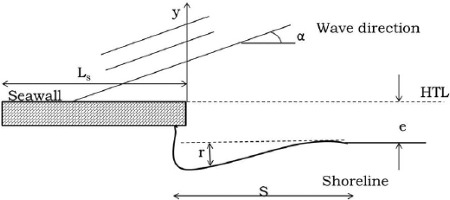
Sketch of seawall for which erosion takes place behind the wall.

It is evident that hard structures can result in severe consequences, thus, it becomes essential to understand the impact of hard stabilization methods, particularly seawalls on beaches, which forms the main objective of this article. In this research, a combination of numerical modelling (Manek and Balaji, 2014) and analytical modelling is used to predict the end-wall effect which is validated with in-situ measurements. Furthermore, the total longshore sediment transport rate per year along the selected coast is also estimated, based on an established theoretical model. Independently, high-resolution satellite datasets are used to study the shoreline changes that have taken place after the seawall was constructed along the coastal region of Fansa, Gujarat, India.

Study area

The study region (Figure 2) is located along the coastal village of Fansa (72° 47′ 39.39″E, 20° 21′ 06.35″N), in the district of Valsad, Gujarat, which adjoins the Arabian Sea. A rubble-mound seawall with a total length of 900 m was constructed along this coastline in the year 2011 to protect the shoreline against wave attack and subsequent erosion.

Figure 2.

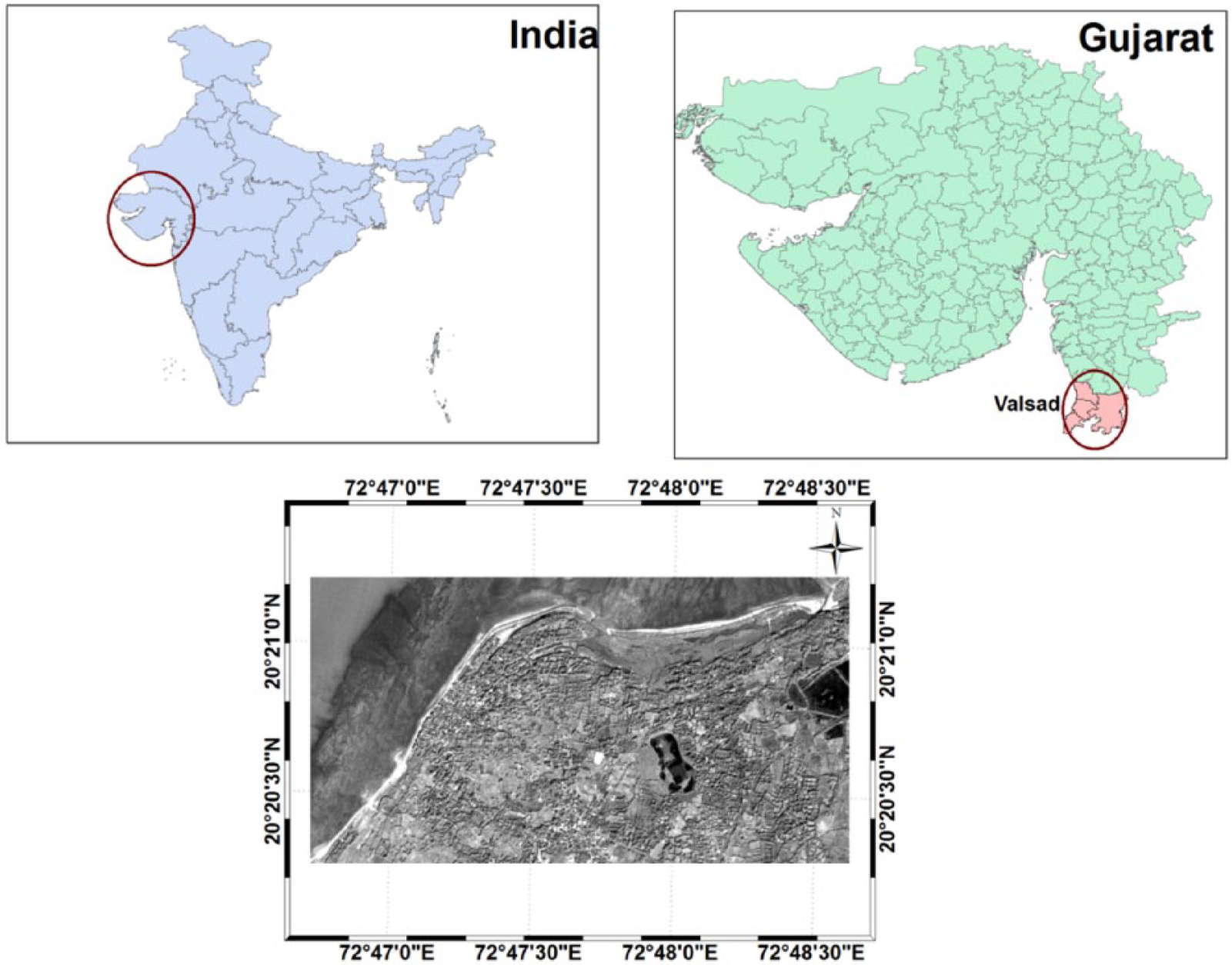
Study area – Fansa Coastline, South Gujarat.

Data and methodology

Data collection

The flanking effect of seawall, along the coast of Fansa, is measured by tracing the high tide line (HTL) and low tide line (LTL) using a handheld global positioning system GPS (Trimble GeoXT). Figure 3 represents the typical view of the strategy followed to carry out beach profile in-situ measurements in front of the seawall and also at the end of the wall along the coastline for August 2012. As can be seen in Figure 4, the seawall along the Fansa coast is a rubble-mound seawall which has resulted in the flanking of the shoreline (Figure 5).

Figure 3.

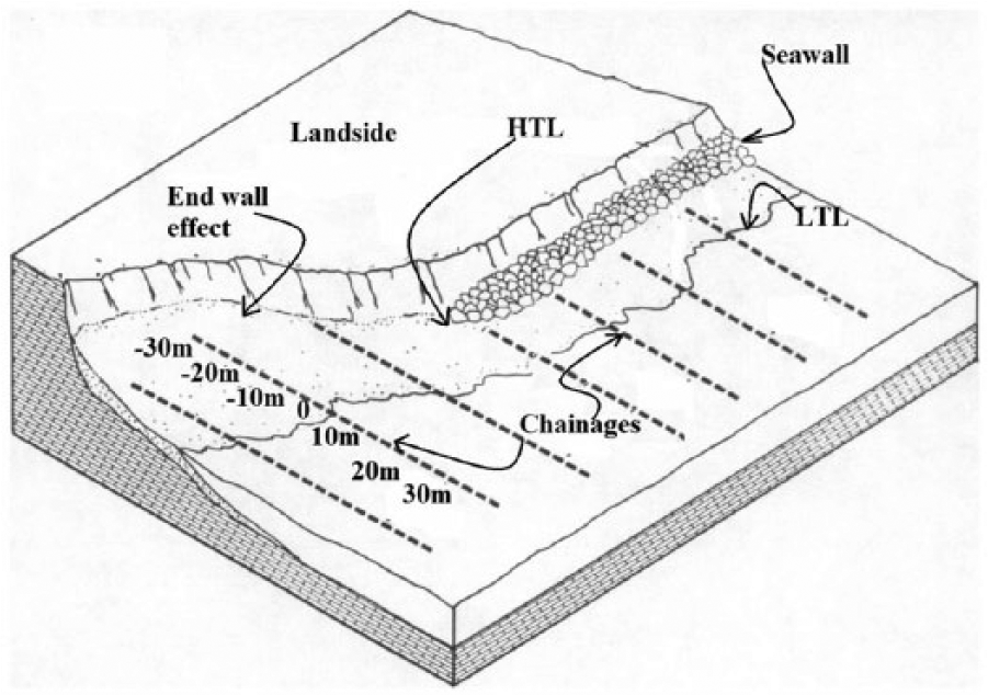
Schematic sketch representing the typical view of in-situ measurements.

Figure 4.

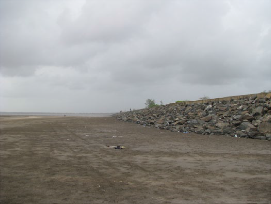
Typical view of beach and rubble-mound seawall along the Fansa coast.

Figure 5.

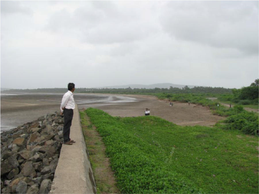
Typical view of the flanking at the end of the seawall.

RS datasets

Temporal CARTOSAT 1 PAN data of comparable season and tidal elevation are selected to estimate the shoreline changes along this region. Data of spatial resolution of 2.5 m for 13 January 2011, 15 January 2012 and 7 December 2014 with Universal Transverse Mercator (UTM) zone 43 north projection systems are used for this analysis.

Methodology

Numerical model – wave transformation study

Generally, near-shore wave propagation is influenced by complex bathymetry, currents, water-level variation and coastal structures. The wave transformation study (Manek and Balaji, 2014) is conducted using STWAVE (Anderson and Smith, 2014; Massey et al., 2011), developed by the US Army Corps of Engineers. STWAVE is a steady-state finite difference model based on the wave action balance equation that calculates wave spectra on a rectangular grid. This wave transformation study helps to estimate the wave parameters between offshore and near-shore of the selected coast, and the results obtained from this are further used in the analytical model.

Analytical model – Parabolic shape model

Headland bay beaches of varying sizes and shapes exist at the down-drift side of protruding natural or man-made (seawall, jetty, etc.) headlands. Since 1940, scientists are trying to establish an empirical expression to fit part or whole of the bay periphery. Parabolic shape model (Hsu and Evans, 1989) is one such empirical model which represents the shape of the equilibrium very well on the down-drift side. This model relates the shoreline changes to the tip of an up-drift headland or wave diffraction point, by virtue of which it is possible to assess the relocation of the up-drift control by man-made structures (i.e. seawall and detached breakwaters).

This parabolic relationship is used to check the stability of the crenulated-shaped bays, as this model performs fairly well in representing the static equilibrium plan form of the fully developed crenulated-shaped beaches. The advantage of using parabolic model is that it is applicable in tidal seas and can represent the high- and low-tide coastlines. However, the model is not capable of predicting the equilibrium plan form in the coastlines, which are close to the tidal inlets due to the dynamical characteristics of sediment transport. In addition, this model cannot predict the effect of obstacles, such as islands, on the beach formations that are located slightly away from the coastline. Figure 6 shows the definition sketch of the parameters associated with parabolic shape model

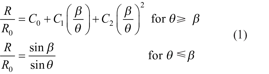
\begin{array}{l} \frac{R}{R_{0}} = C_{0} + C_{1} (\frac{β}{θ}) + C_{2} {(\frac{β}{θ})}^{2} for θ ⩽ β \\ \frac{R}{R_{0}} = \frac{\sin β}{\sin θ} for θ ⩾ β \end{array}

(1)

where R is the radius of the curve at an angle θ; R₀ is the radius to the control point (transition point between the curved part of the bay and the straight part that is parallel to the incoming waves); β is an angle defining the bay shape; θ is an angle between incoming wave crests and radius line R; and C₀, C₁ and C₂ are the coefficients determined as functions of β.

Figure 6.

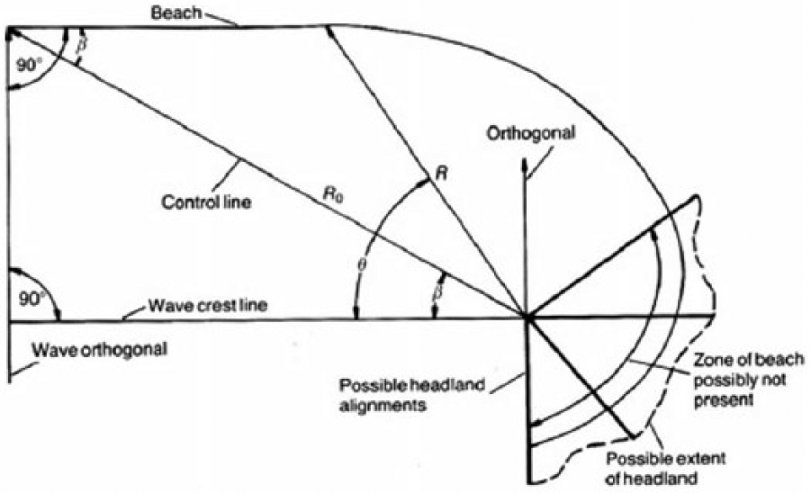
Definition sketch of variables employed in parabolic solution of bays (Hsu and Evans, 1989).

Parameters used

Assessment of beach shape at the end of seawall at Fansa requires near-shore wave, sediment and beach characteristics as priori. The results of an earlier wave transformation study (Manek and Balaji, 2014) were used to arrive at the near-shore wave characteristics, such as breaker angle (α_b = 3.5°) and breaking wave height (H_b = 1.5 m). Based on the in-situ measurements, the beach slope along the Fansa coast is in the order of 1:800 to 1:900 (flat beach), which gives the breaker index value, κ as 0.78. Based on the constructed seawall, beach berm height above still water level (SWL; d_b = 4 m) and depth of appreciable sand transport from SWL (d_c = 4 m) are measured. From a simple sediment sample analysis, the porosity is estimated (n = 0.4).

Beach-shape assessment at end of seawall

The control points are selected as (1) the seawall edge and (2) a point along the coastline without any erosion protection structure along it. The shape of the beach now depends on the angle of the wave crest and the line joining the control points. For this, the shoreline orientation is defined and the predominant wave direction, as well as the wave characteristics, is obtained from the transformation studies, as explained earlier. Using these data, the possible coastline recession due to the constructed seawall is estimated.

The estimation is, then, cross verified with another analytical shoreline changes model (Larson et al., 1987, 1997) proposed for end effects of coastal structures. The position of shoreline is given, by the analytical model, as

y = 2 \sqrt{ε t} \tan (α_{b}) {\begin{cases} \frac{1}{\sqrt{π}} \exp [- {(\frac{x}{2 \sqrt{ε t}})}^{2}] \\ - \frac{x}{2 \sqrt{ε t}} e r f c (\frac{x}{2 \sqrt{ε t}}) \end{cases}}

(2)

where

ε = \frac{K H_{b}^{2} C_{g b}}{8} (\frac{ρ}{ρ_{s} - ρ}) (\frac{1}{1 - n}) (\frac{1}{d_{B} + d_{C}})

(3)

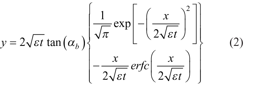
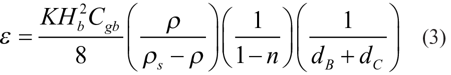
where d_B is the beach berm height above SWL which is measured from SWL, d_c is the depth of appreciable sand transport as measured from SWL, α_b is the breaker angle, H_b is the breaker height, C_gb is the group speed, t is the time period, x is the alongshore coordinate in metres, K is the constant, ρ_s is the density of the sand, ρ is the density of the water, n is porosity and erfc is the error function.

RS & GIS based study - Shoreline changes

CARTOSAT PAN satellite datasets are used to estimate the variations in shorelines of different years. Vectorization technique is applied to get the shoreline features of the years 2011, 2012 and 2014 in the ArcGIS 10 environment. This is further used as an input to the DSAS tool to estimate the rate of shoreline changes, which is calculated based on measured differences between shoreline positions through time. The DSAS tool basically estimates the net shoreline movement (NSM) and end point rate (EPR) which are used to derive the output maps of this study. The NSM calculates the distance between the oldest and the youngest shoreline for each transect, and the EPR is obtained by dividing the NSM, by the number of years elapsed between the two shoreline positions. The linear extents with negative NSM or EPR values indicate erosion, whereas those with positive values indicate accretion.

Results and discussion

Analytical modelling–based analysis

A maximum landward erosion of 20 m and alongshore influence of the erosion of 200 m (Figure 7) is estimated from the parabolic model, on the northern end of seawall, for the first 1 year after completion of the construction. This landward erosion may further extend up to another 20 m by 2014 and may then eventually stabilize. A comparison of the estimated landward erosion with the in-situ measurements conducted during the site visit is found to be in agreement with each other. Parabolic shape model estimation is cross verified with the beach-shape assessment method using equations (2) and (3). From this beach-shape assessment method, change in adjacent shoreline at the end of seawall is predicted to be around 23 m which is comparable with the parabolic shape model results.

Figure 7.

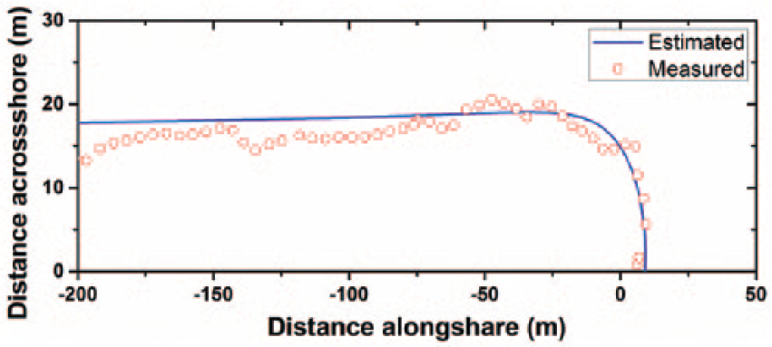
Comparison of measured and estimated parabolic shape view of end-wall effect.

It is understood from the earlier studies that the South Gujarat coast experiences a high sediment transport of the order of 1.5–2 Mm³ (Nayak and Chandramohan, 1992). Specifically along the Valsad coast, the estimated southerly and northerly sediment transports are 0.594 and 0.98 Mm³, respectively. It is clear from the numerical model estimates that the northerly sediment drift is more, and hence, the annual net sediment transport along the Valsad coast is expected to be towards the north direction. It is also reported that large monthly sediment transport is generally observed to be during southwest monsoon, which is about 2.3 × 10⁶ m³ (Nayak and Chandramohan, 1992). In this study, using CERC (US Army Corps of Engineers, 2002) equation, the estimated longshore sediment transport rate is of the order of 1.9 × 10⁶ m³ per year along Fansa coast providing evidence of end-wall effect on the northern side.

RS & GIS based analysis

The RS analysis is carried out independently to understand the shoreline change dynamics of this region. In the satellite dataset of 2011, only an incomplete seawall is seen, which is observed to be completed in the satellite imagery of 2012. Based on the visual analysis, it can be seen in Figure 8 that approximately 250–300 m of the shoreline, north of the seawall, for the year 2014, has completely eroded due to the construction of the hard structure. Moreover, it is interesting to observe that from 2011 to 2014, the landward erosion in the immediate vicinity of the down-drift direction of the seawall is approximately 40 m, which is also predicted by the analytical model.

Figure 8.

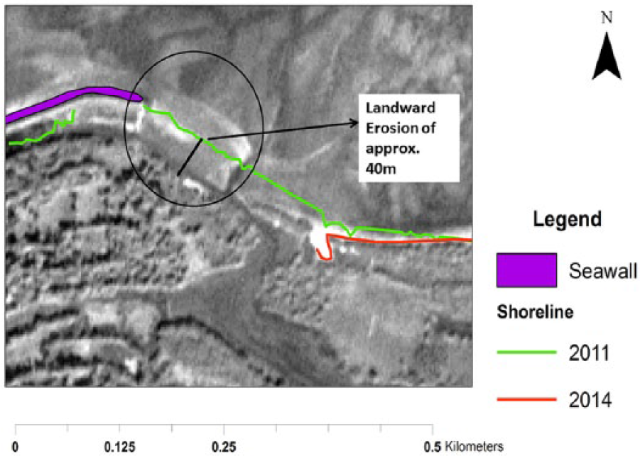
Landward erosion from 2011 to 2014.

Furthermore, a shoreline erosion analysis (Figure 9) is carried out for the coastline along the northern side approximately 250 m away from the end of the seawall to qualitatively and quantitatively understand the effects of the installation. It is estimated that the average EPR is approximately about 0.417 m/year and the average NSM is 1.63 m.

Figure 9.

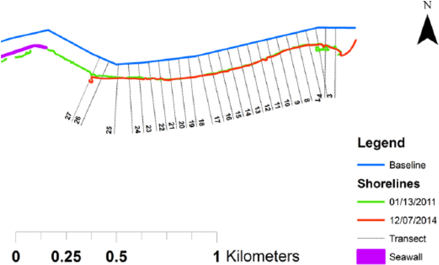
Shoreline change analysis.

An important advantage of RS especially in this study is that it provides a snapshot of the temporal, as well as spatial, changes that take place over a period of time. Hence, using CARTOSAT 1 imagery, it has been possible to understand the effect of the seawall in the adjoining region post construction. Another important observation that is witnessed in the satellite datasets (Figure 10) is that the high sediment deposition in this region has caused a decrease in the size of the river mouth in the 2014 image, resulting in the narrowing of the channel (encircled in red) that allows the water to flow inland. As discussed in the previous section, the longshore sediment transport in this region is reportedly northward, and hence, the change in the sediment transport dynamics due to the seawall construction can be hypothesized to have some impact on the adjoining river mouth as can be seen clearly in the images. In order to verify this observation, it is imperative to conduct a thorough investigation with the help of numerical modelling; however, this can be considered as a reasonable inference as no changes are seen in the year 2011 and 2012, but only in 2014.

Figure 10.

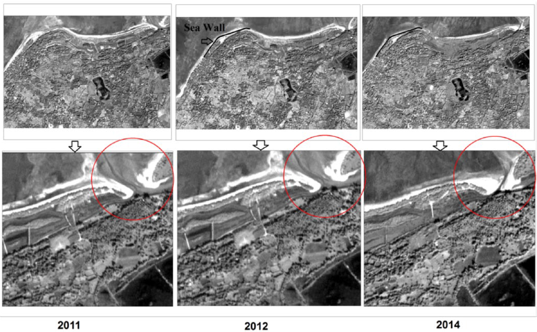
Changes in river mouth configuration.

Finally, it can be suggested that sediment mobilization, wave reflection causing sediment transport, refraction and diffraction are some of the commonly cited processes involved in the seawall–beach interaction (Tait and Griggs, 1991). Much of the end scour observed here is triggered due to alongshore sediment transport caused by reflecting waves in an alongshore direction, as well as refraction and diffraction. In this study, the effects of seawall are seen in the form of scouring, change in sediment dynamics and shoreline changes in the adjoining regions.

Conclusion

In the present times, there has been considerable change in the approach to coastal management by virtue of the improvement in the understanding and knowledge of coastal dynamics and shoreline erosion. Very often, the detrimental effects of seawall construction are overlooked in order to preserve the beach and to control the irresponsible shoreline development that takes place along it.

In this study, an effort has been made to understand the effects of seawall construction using a combination of numerical and analytical modelling and geo-informatics. It is evident that the construction of seawall along the coast of Fansa has resulted in a landward erosion of about 20 m in the down-drift direction of the seawall, within a year of construction. Based on a theoretical model, the beach is further predicted to erode by another 20 m before attaining the state of equilibrium by the year 2014. This estimation is successfully validated through an RS-based analysis, the results of which confirm that the landward erosion from 2011 to 2014 is approximately 40 m in the northern side of the sea wall.

Although the beach along the coast of Fansa is predicted to have already stabilized, the construction of seawall has evidently caused some changes in the shoreline morphology. It is important to understand that although the construction of hard structures allows for the protection of the property by controlling the beach and bluff erosion, this kind of fortification reduces the natural delivery of sand leading to detrimental effects in the down-drift coast beaches. This study highlights the need to examine the seawall–beach interaction on a case-by-case basis, so that a more informed decision can be made while installing a hard structure to control shoreline erosion.

Footnotes

Funding

The author(s) received no financial support for the research, authorship and/or publication of this article.

Author biographies

Dr. Balaji, R is an Associate Professor in the Department of Civil Engineering of Indian Institute of Technology Bombay (IITB), India. He has earned his MS and PhD from the Department of Ocean Enginerring, IIT Madras. His research area of interest are Coastal engineering, numerical and physical modeling of coastal processes (tidal hydrodynamics & wave transformation), Wave and Tidal Energy, wave-structure interaction.

Mr. Sathish Kumar, S is a doctoral student in the Civil Engineering department of Indian Institute of Technology Bombay. His research area of interest are tidal hydrodynamics, Oil-spill modelling.

Ms. Ankita Misra is a CSIR- SRF, doctoral student in the Civil Engineering department of Indian Institute of Technology- Bombay (IIT-B). Her work mainly involves application of remote sensing (RS) and GIS in coastal studies.

References

Anderson

Smith

(2014) Wave attenuation by flexible, idealized salt marsh vegetation. Coastal Engineering 83: 82–92.

Bhattacharya

Sarkar

Bhattacharya

(2003) An assessment of coastal modification in the low lying tropical coast of north east India and role of natural and artificial forcings. In: Proceedings of international conference on estuaries and coasts, Hangzhou, China, 9–11 November.

CERC, US Army (1984) Shore Protection Manual. Washington, DC: US Army Corps of Engineers.

Choudhary

Gowthaman

SanilKumar

(2013) Shoreline change detection from Karwar to Gokarna-South West coast of India using remotely Sensed data. International Journal of Earth Sciences and Engineering 6(3): 489–494.

Griggs

Tait

(1988) The effects of coastal protection structures on beaches along northern Monterey Bay, California; The effects of seawalls on the beach. Journal of Coastal Research 4(4): 93–111.

Gupta

(2014) Monitoring shoreline changes in the Gulf of Khambhat, India during 1966–2004 using RESOURCESAT-1 LISS-III. Open Journal of Remote Sensing and Positioning 1(1): 27–37.

Hall

Pilkey

(1991) Effects of hard stabilization on dry beach width for New-Jersey. Journal of Coastal Research 7(3): 771–785.

Hegde

(2010) Coastal erosion and mitigation methods—global state of art. Indian Journal of Geo-Marine Sciences 39(4): 521–530.

Hsu

JRC

Evans

(1989) Parabolic bay shapes and applications. Proceedings of the Institution of Civil Engineers 87(4): 557–570.

10.

Hsu

JRC

Silvester

Asce

(1996) Stabilizing beaches downcoast of harbor extensions. Coastal Engineering 25: 3986–3999.

11.

Hsu

JRC

Lee

et al . (2010) Static bay beach concept for scientists and engineers: A review. Coastal Engineering 57(2): 76–91.

12.

Jayappa

Vijaya Kumar

Subrahmanya

(2003) Influence of coastal structures on the beaches of southern Karnataka, India. Journal of Coastal Research 19: 389–408.

13.

Kraus

(1988) The effects of seawalls on the beach: An extended literature review. Journal of Coastal Research SI(4): 1–28.

14.

Kumar

Jayappa

(2009) Long and short-term shoreline changes along Mangalore coast, India. International Journal of Environmental Research 3(2): 177–188.

15.

Kumar

Ravinesh

(2011) Will shoreline armouring support marine biodiversity? Current Science 100(10): 1463.

16.

Larson

Hanson

Kraus

(1987) Analytical Solutions of the One-Line Model of Shoreline Change. Washington, DC: US Army Corps of Engineers.

17.

Larson

Hanson

Kraus

(1997) Analytical solutions of one-line model for shoreline change near coastal structures. Journal of Waterway, Port, Coastal, and Ocean Engineering 123(4): 180–191.

18.

McDougal

Sturtevant

Komar

(1987) Laboratory and field investigations of the impact of shoreline stabilization structures on adjacent properties. In: Coastal sediments, May 1987, New Orleans, LA, American Society of Civil Engineering, pp. 961–973.

19.

Manek

Balaji

(2014) Assessment of shoreline oscillations along south Gujarat coastline, India. Indian Journal of Marine Sciences 43: 1281–1285.

20.

Mani

(2001) A coastal conservation programme for the Chennai sea shore, India – A case study. Journal of Coastal Conservation 7(1): 23–30.

21.

Massey

Anderson

Smith

et al . (2011) STWAVE: Steady-state spectral wave model, version.6.0. ERDC/CHL-SR-11-1, September. Vicksburg, MS: US Army Corps of Engineers Engineer Research and Development Center.

22.

Misra

Balaji

(2015) Decadal changes in the land use/land cover and shoreline along the coastal districts of southern Gujarat, India. Environmental Monitoring and Assessment 187(7): 461.

23.

Mukhopadhyay

Mukherjee

Hazra

et al . (2011) Sea level rise and shoreline changes: A geoinformatic appraisal of Chandipur coast, Orissa. International Journal of Geology, Earth & Environmental Sciences 1(1): 9–17.

24.

Murali

Dhiman

Choudhary

et al . (2015) Decadal shoreline assessment using remote sensing along the central Odisha coast, India. Environmental Earth Sciences 74(10): 7201–7213.

25.

Nayak

Chandramohan

(1992) A longshore sediment transport estimation for the Indian coast. In: Swamy

Das

Anthony

(eds) Physical Processes in the Indian Sea. Proceedings of First Convention of ISPSO. Goa, India: National Institute Oceanography, pp. 111–116.

26.

Neelamani

Sundaravadivelu

(2006) Erosion, protection of Pondicherry coast, southeast India. Journal of Coastal Research (special issue) 39: 880–883.

27.

Pilkey

Wright

III (1988) Seawalls versus beaches. Journal of Coastal Research (special issue) SI(4): 41–64.

28.

Pilkey

Cooper

JAG

(2012) “Alternative” shoreline erosion control devices: A review. In: Pitfalls of Shoreline Stabilization. Netherlands: Springer, pp. 187–214.

29.

Sheik

Chandrasekar (2011) A shoreline change analysis along the coast between Kanyakumari and Tuticorin, India, using digital shoreline analysis system. Geo-Spatial Information Science 14(4): 282–293.

30.

Tait

Griggs

(1991) Beach Response to the Presence of a Seawall; Comparison of Field Observations. Washington, DC: US Army Corps of Engineers.

31.

US Army Corps Of Engineers (2002) Coastal Engineering Manual. Engineer Manual 1110-2-1100. Washington, DC: US Army Corps of Engineers.

Understanding the effects of seawall construction using a combination of analytical modelling and remote sensing techniques: Case study of Fansa,Gujarat,India

Abstract

Keywords

Introduction

Seawall and its influence on the beach

Beach response

End scour/flanking

Study area

Data and methodology

Data collection

RS datasets

Methodology

Numerical model – wave transformation study

Analytical model – Parabolic shape model

Parameters used

Beach-shape assessment at end of seawall

RS & GIS based study - Shoreline changes

Results and discussion

Analytical modelling–based analysis

RS & GIS based analysis

Conclusion

Footnotes

Funding

Author biographies

References