
Abstract
Fluid equations in Computational Fluid Dynamics coupled with Discrete Element Method (CFD-DEM) simulations solve the volume-averaged Navier–Stokes equations. Full coupling between the dispersed phase and continuous phase is made by the exchange of source terms as well as the void fraction. The void fraction is calculated from the presence of the particles in the computational fluid cells while the source terms are calculated from the point mass force models of the fluid–particle interaction forces. Dense particulate system with large spatiotemporal variations in the void fraction shows hard convergence behavior. This can impact the robustness of the solver during the time integration process. One option is to use partial coupling by neglecting the explicit effect of void fraction in the fluid momentum equations while retaining its effect on force models. Although the partial coupling is more stable and shows better convergence behavior, the mobility of the particles is found to be reduced as compared to the full-coupling approach. In the current work, we propose a revised partial coupling in which a modified fluid velocity is used in point mass force models to compensate for the omission of the void fraction in the fluid governing equations. The effectiveness of this method is demonstrated in a fluidized bed and in sediment transport simulations. In both cases it is shown that the use of the proposed method gives very good comparisons with the fully coupled simulations while reducing the fluid calculation time by factors ranging from 1.35 to 4.35 depending on the flow conditions. The revised partial coupling is not recommended as a substitute for full coupling in dense systems but as an alternate approach when full coupling leads to numerical difficulties.
Introduction
Two methods are typically used to simulate particulate flow systems, namely the Eulerian–Eulerian approach and the Eulerian–Lagrangian approach. In the first method, also known as the two-fluid model (TFM), both phases are modeled as two interpenetrating fluids using two sets of conservation equations. The latter method solves the volume-averaged Navier–Stokes equations of the continuous phase while the particles are tracked by solving a dynamic equation based on Newton’s second law of motion. Forces on each particle can be either solved by performing integration over the surface (resolved flow simulations) or by using point mass force model (discrete element method). The TFM is appealing since it allows for simulating industrial and natural scale systems.1,2 This is because modeling the dispersed phase as a fluid is much less expensive than the burden of tracking a large number of particles. However, modeling the dispersed phase as a continuum requires additional closure models (e.g. to estimate the solid viscosity) and the method is problematic when simulating particles with significant size or shape distribution or when handling particle–wall collision. 3
Although the Eulerian–Lagrangian approach includes a better representation of the physics, its application to industrial and to natural scales is impractical due to the large number of particles involved and the computational cost. The cost of Eulerian–Lagrangian approach (particle resolved simulations and CFD-DEM) scales with the number of particles to be simulated. Particle-resolved simulations require a fluid grid that is at least one order of magnitude finer than the particle diameter and thus the method is quite restrictive in the size of the system that can be simulated. Simulation of thousands of particles using resolved flow simulation is reported for turbulent channel flow 4 and fluidized bed 5 applications. CFD-DEM, on the other hand, uses point mass particles and the particle forces are modeled. While millions of particles have been simulated using the CFD-DEM method when using large number of processors with efficient parallelization techniques,6–8 large system simulations are not that common. Thus, it is important to reduce the cost of CFD-DEM simulations without sacrificing accuracy. One method that is used is to lump a group of particles into representative particles (swarms or parcels) to reduce the number of particles. In such simulations quick, but somewhat less accurate, estimates can be obtained. 9
At dilute concentration of the dispersed phase (volume concentration of the dispersed phase <1 × 10⁻³) interaction forces between the particles can be neglected resulting in two-way coupling between the fluid and the particles. 10 In this case the particles are coupled to a single-phase flow solver using drag forces. At even lower concentration of particles (volume concentration of the dispersed phase <1 × 10⁻⁶) the feedback from the particles to the fluid can be further neglected resulting in one-way coupling. At dense concentration of the dispersed phase (>1 × 10⁻³) the interaction between the particles becomes important. The term four-way coupling is used to indicate that the particle–particle interaction force becomes important in addition to the two-way coupling. 10
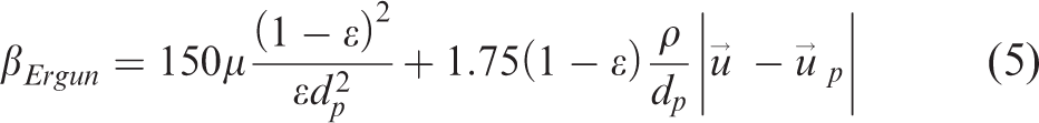
The volume-averaged Navier–Stokes equations are typically used for dense particulate flow systems. 11 Not only is the fluid momentum affected by the forces exerted on the particles but also by the flow blockage or solid fraction due to the presence of particles. Additionally, the point mass force models (e.g. drag) are also affected by the flow blockage (e.g. Sangani et al. 12 and Wen 13 ). Thus for dense systems, the solid fraction or its complement, the void fraction, plays a critical role in prediction of dynamics. To satisfy the volume-averaged basis of the Navier–Stokes and continuity equations, the calculation of the void fraction should be over a sufficiently large sample of particles to not only give some measure of statistical convergence but also to have a smooth spatial and temporal distribution of the void fraction. Some researchers suggest that the size of the computational cell over which the fluid void fraction is averaged to be ∼3–4 times that of the particle diameter.14,15 Many other researchers use higher ratios for consideration of the computational cost (e.g. Kerst et al. 16 and Zou et al. 17 ). The method of calculating the void fractions in the computational cell can be different as some researchers assume that the full particle is located inside the computational cell in which its center resides (particle center method (PCM)) 18 whereas others use only portions (or sectors) of the particle of the volume size that is physically located in the cell (exact method). 19 The exact method is more accurate but more expensive compared to the PCM. An alternative method (offset method) for calculating the void fraction was suggested by Alobaid et al. 20 in which the void fraction is calculated by averaging the cell center method results in multiple spatially offset cells. The offset method is reported to improve the accuracy of the predication of the void fraction compared to the PCM.21,22 Peng et al. 23 reported that PCM produces the same results as the exact method if the cell to particle diameter ratio is 3.82. Peng et al. 23 also reported that the void fraction averaging becomes unsuitable if the cell size is smaller than 1.63 of the particle diameter.
In instances when the fluid grid needs to be of the same order or smaller than the particle diameter, such as in wall-bounded turbulent flows, the void fraction can be either calculated on a coarser particle grid that is mapped over the existing fluid grid 24 or smoothed over the neighboring region.8,25 These techniques allow for full coupling between the two phases using particle forces as well as void fractions in the fluid momentum equations. Failure to have a smooth variation of void fraction results in long convergence times of the flow solver at each time step and in extreme cases also leads to numerical instabilities. Smoothing the void fraction over a wider support using different techniques is found to have a negative impact on the results. 26
Many past studies in the field of sediment transport have avoided fully coupled simulations because of the inconsistency posed by the volume-averaging assumption and the need to resolve near-wall turbulence.27–30 In these studies, the dispersed phase was coupled through source terms to a single-phase flow solver. Although this approach is not commonly used in energy applications (i.e. fluidized and spouted bed and raiser), Wu et al. 31 adapted similar strategy when they coupled DEM to a commercial unstructured flow solver. Additional source terms were added to the governing equations in an attempt to account for the presence of the particles. The implementation is found to capture the important characteristics at the specified operating condition. Further improvement to the proposed source terms was performed by Wu et al. 32 in order to ensure conservation of mass of the implementation.
The differences between coupling the disperse phase to a multiphase flow solver (full coupling) and coupling the particles to a single-phase flow solver (will refer to this as the “base partial coupling”) was investigated by Elghannay and Tafti 33 in sediment transport under turbulent conditions. The fully coupled method solved the volume-averaged Navier–Stokes equations including the effect of void fraction and drag forces from the solid phase. In partial coupling, the void fraction was not considered (defaulted to unity) and only the drag forces were fed back to the fluid momentum balance. It was found that the partial coupling tended to underpredict the mobility of the particles resulting in lower sediment transport compared to full coupling when the same void fraction-sensitized drag model is used for both. The deviation increased as more particles were transported as the bed transitioned from the bedload regime to suspended load. So on one hand, full coupling leads to complications in the calculation of void fraction and numerical difficulties during time integration of fluid equations, while on the other hand, partial coupling eliminates these difficulties but reduces accuracy.
In this paper we suggest a method to bridge the difference between the partial coupling and the full-coupling techniques. Admittedly, the proposed modified partial coupling (will be referred to as the revised partial coupling) is still an approximation to the four-way full coupling, but it is shown that using the proposed method gives very close quantitative agreement with fully coupled simulations at a lower computational cost. Thus, the proposed method should be viewed as a significant improvement over the base partial coupling rather than a substitute for the fully coupled method. It does not replace the fully coupled method but can be viewed as a reasonably accurate substitute when the fully coupled method poses numerical difficulties and partial coupling is the only viable alternative. A comparison of the performance of the three coupling techniques is provided on two different applications. The differences in instantaneous and averaged results are discussed along with the computational savings.
Mathematical formulation
Particle dynamic equation
In DEM the path of each particle is predicted by the integration of its equation of motion resulting from the application of Newton’s law of motion. The equation of motion of particles moving under influence of drag (

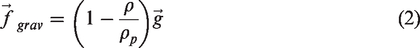
The gravity force includes both gravity and buoyancy effects. The submerged weight of the particle (per unit mass of the particle) is given by


The blending function W is defined as

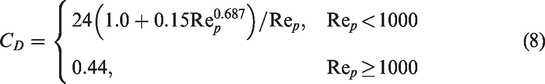
In equation (9) μ is the dynamic viscosity of the fluid.
Fluid equations
The carrier phase is modeled using the volume-averaged Navier–Stokes equations
11
derived for multiphase flows. The current implementation of the continuous phase is governed by Model B of Lu et al.
34
in which the pressure drop is accounted for only by the fluid. The fluid equations are written as

The flow field is solved on a nonstaggered finite-volume grid using a semi-implicit fractional step method. The flow field is advanced in time using the calculated void fractions and drag forces from the previous time step. The calculated fluid velocity field is transferred to the particle grid and the particles are advanced in time. During this process, the continuous and disperse phases are coupled via the drag force and void fractions. The void fractions and cumulative particle drag forces are calculated in each particle grid cell and transferred to the fluid grid for use in equations (3) to (9). The void fraction is calculated by a weighted distribution of particle volumes in a given particle grid cell to the cell vertices and then averaging the cumulative volumes from the vertices to the fluid cells contained in the particle cell. A similar procedure is carried out for transferring the cumulative drag forces from the particle to the fluid grid. A detailed description of the dual-grid formulation is described in Deb and Tafti. 24
Another technique, which is used in the sediment transport simulations is the use of substepping. In this technique, the particle is advanced multiple time steps during a fluid time step (Δtp =Δtf/Nsub, where Δtp is the time step used for the particle calculation, Δtf is the fluid time step, and Nsub is the number of particle substeps within a fluid time step). Linear interpolation is used to approximate the fluid velocity between nΔtf and (n + 1)Δtf, where n indicates the number of the fluid time step. Using this technique relaxes the simulation from being advanced in time using the strict time scale imposed by the collision time scale.
Base and revised partial coupling
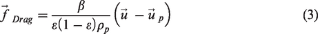
In the base partial coupling, the void fraction is assumed to be unity (ε = 1) in equations (10) and (11) while the conventionally calculated void fraction is used in the drag force model. As mentioned in the “Introduction” section, the base partial coupling was found to consistently underpredict the mobility of the particles. It was reasoned that the underprediction was caused by a lower drag force on particles. This was attributed to the realization that the interstitial fluid velocity (u) used in the drag force (equation (3)) was being underpredicted in the absence of the void fraction in the fluid momentum equations. In effect, what was being calculated was the superficial velocity (U= ε.u). Thus, it was postulated that the underprediction of particle mobility when using partial coupling could be bridged if the velocity calculated during partial coupling is corrected using the void fraction of the fluid. The base partial coupling uses a void fraction of 1 in equations (10) and (11) and an uncorrected relative velocity
Simulation details and results
Bubbling fluidized bed
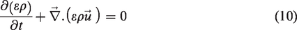
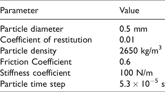
As an extreme case of a dense fluid–particle system, a fluidized bed experiment 14 at a superficial velocity of 0.9 m/s is selected to test the revised partial coupling. The intent here is not to recommend the revised partial coupling over full coupling, but to show that the method gives reasonable results in the extreme case of a fluidized bed. The selected velocity is three times the minimum fluidization velocity. The simulated fluidized bed has a width, depth/transverse thickness, height of 44 mm × 10 mm × 160 mm, respectively. All side walls were set to no-slip boundary condition and the top and bottom wall were set to a permeable wall with velocity equal to the fluidization velocity. The three-dimensional simulation was conducted with 9240 particles on a grid which is 12 × 2 × 32 cells in the x, y, and z directions, respectively. The time step used in all calculation is ∼5 µs and details of the particle properties and modeling parameters are presented in Table 1. Three simulations were conducted using full coupling (equations (10) and (11)), partial coupling, and revised partial coupling techniques.
Simulation parameters used for Muller’s experiment.31
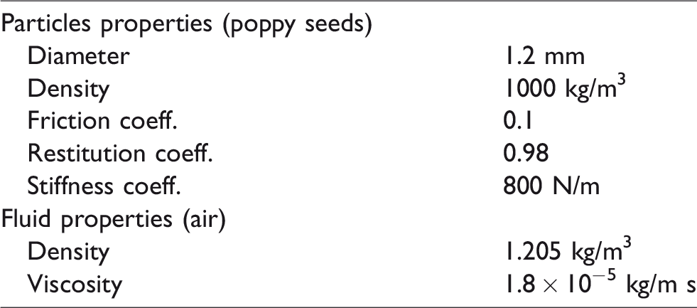
The temporal change of the averaged velocity of all particles is shown in Figure 1. The particles are initialized with the initial fluid velocity which is set to the fluidization velocity (Uf = 0.9 m/s). The particles initially move upward, decelerate under the influence of gravity, and start descending down as their velocity changes from positive to negative. The base partial coupling degenerates to a static bed after its momentum is lost through collisions and the drag force experienced by the particles is not enough to lift the particles. Whereas both the full coupling and the revised partial coupling exhibit a fluctuating average particle velocity in a mobile (bubbling) bed. Both bubbling beds show similar bubbling behavior, a central bubble moves up from the center of the bed followed by a recession of the particles down from the side walls. A velocity signal that ramps up from a negative value to a positive value represents an upward motion of a significant cloud of particles, whereas if the majority of the particles are moving down then the averaged particle velocity will be negative.
Comparison of averaged particles velocity for the different coupling approaches.
All simulations were run for approximately 10 s and the results were averaged for the last 7.5 s. The average void fraction of the three simulations is shown in Figure 2 along with the average solid velocity, which is nondimensionalized with the fluidization velocity. Figure 2 clearly demonstrates that the base partial coupling shows poor comparison with the full-coupling approach. In fact, no fluidization or bubbling is observed in this case. The revised partial coupling, on the other hand, shows almost the same bed height with slightly faster particles in the core of the bed. In spite of the subtle differences between the revised partial coupling and the full coupling, the revised partial coupling shows significant improvement over the base formulation.
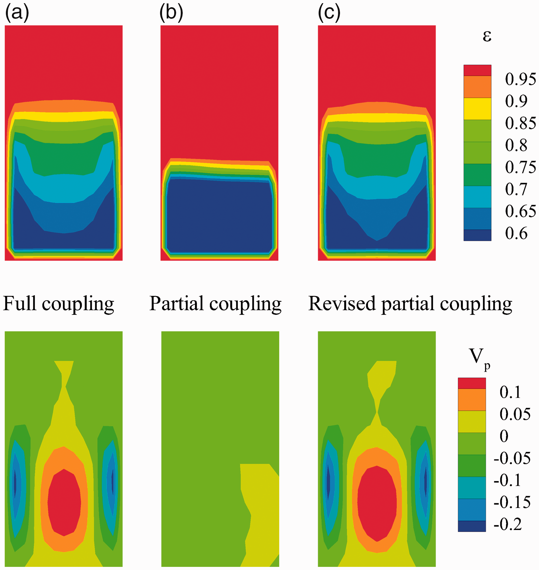
Comparison of averaged void fraction (top) and solids velocity (bottom) for (a) fully coupled simulation, (b) base partial coupling, and (c) revised partial coupling.
Further, a comparison of the current time-averaged results with the work of Müller et al.14,35 is shown in Figure 3 at selected locations above the distributor plate. The results of the averaged void fraction from both the revised partial coupling and the full coupling almost match each other and compare well with the measurements of Müller et al. 14 The base partial coupling, on the other hand, shows low voidage due to the absence of any gas bubbling activity. Both full coupling and the revised partial coupling also match well with the measured time-averaged solid velocity.
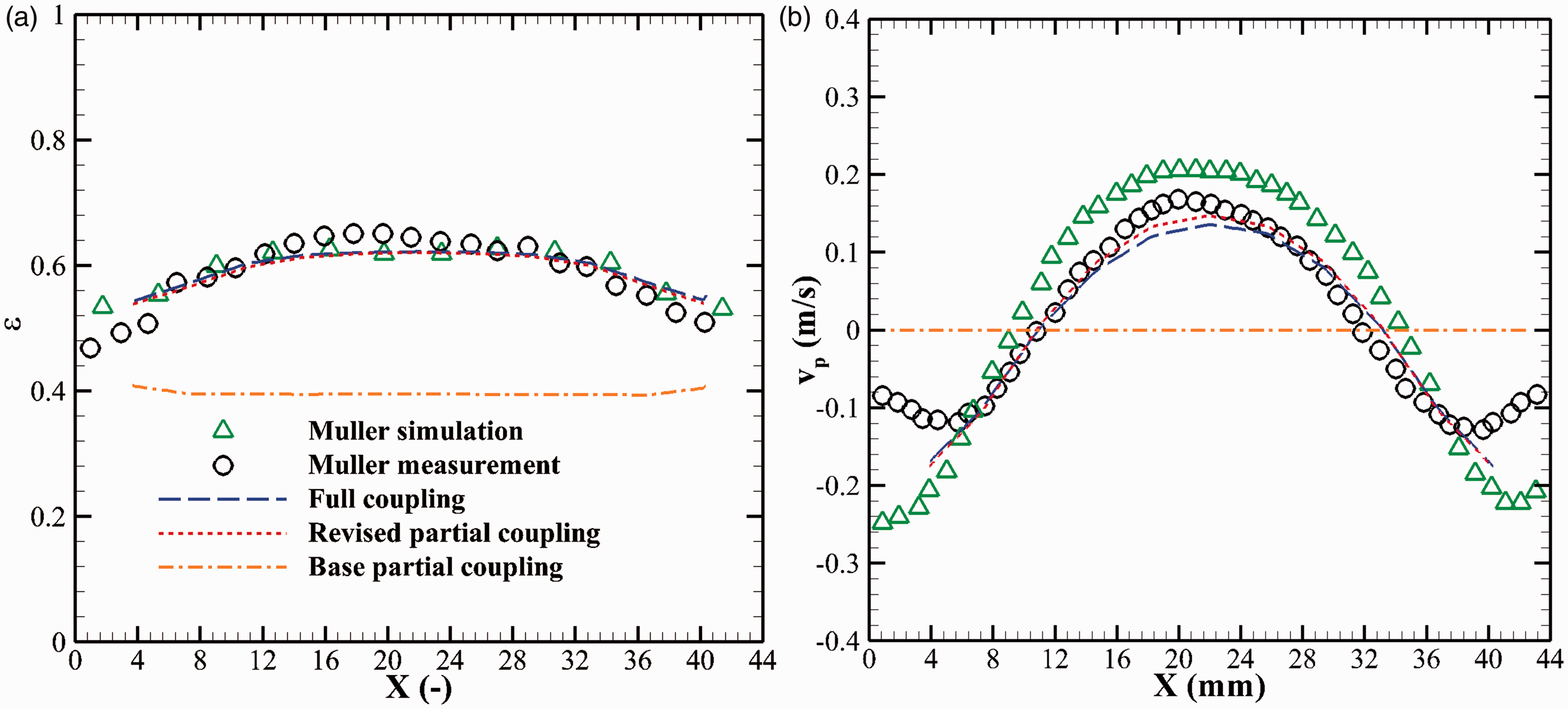
Comparison of time-averaged results of (a) void fraction at 16.4 mm above the distributor plate and (b) solids velocity 25 mm above the distributor plate.
It is also worthwhile to examine the interstitial fluid velocity and the pressure drop from using the different coupling techniques. Figure 4 shows the average fluid velocity (nondimensionalized with respect to the fluidization velocity) obtained using the three coupling techniques. It can be seen that both partial coupling techniques show obvious deviations in the velocity flow field. This is not surprising since the single-phase flow solution does not account for the presence of the particles. However, it is noteworthy that the true interstitial fluid velocity can be recovered from the revised partial coupling by using the predicted void fraction (ucorr = u/ε). Figure 5 presents the comparison of the averaged interstitial velocity flow field of the full coupling and the revised partial coupling together with the distribution of the percentage difference. It can be seen that the corrected interstitial velocity shows reasonably good comparison with the full-coupling interstitial velocity. The difference is limited to ∼10% in most of the domain with small domain of margin error >15%.
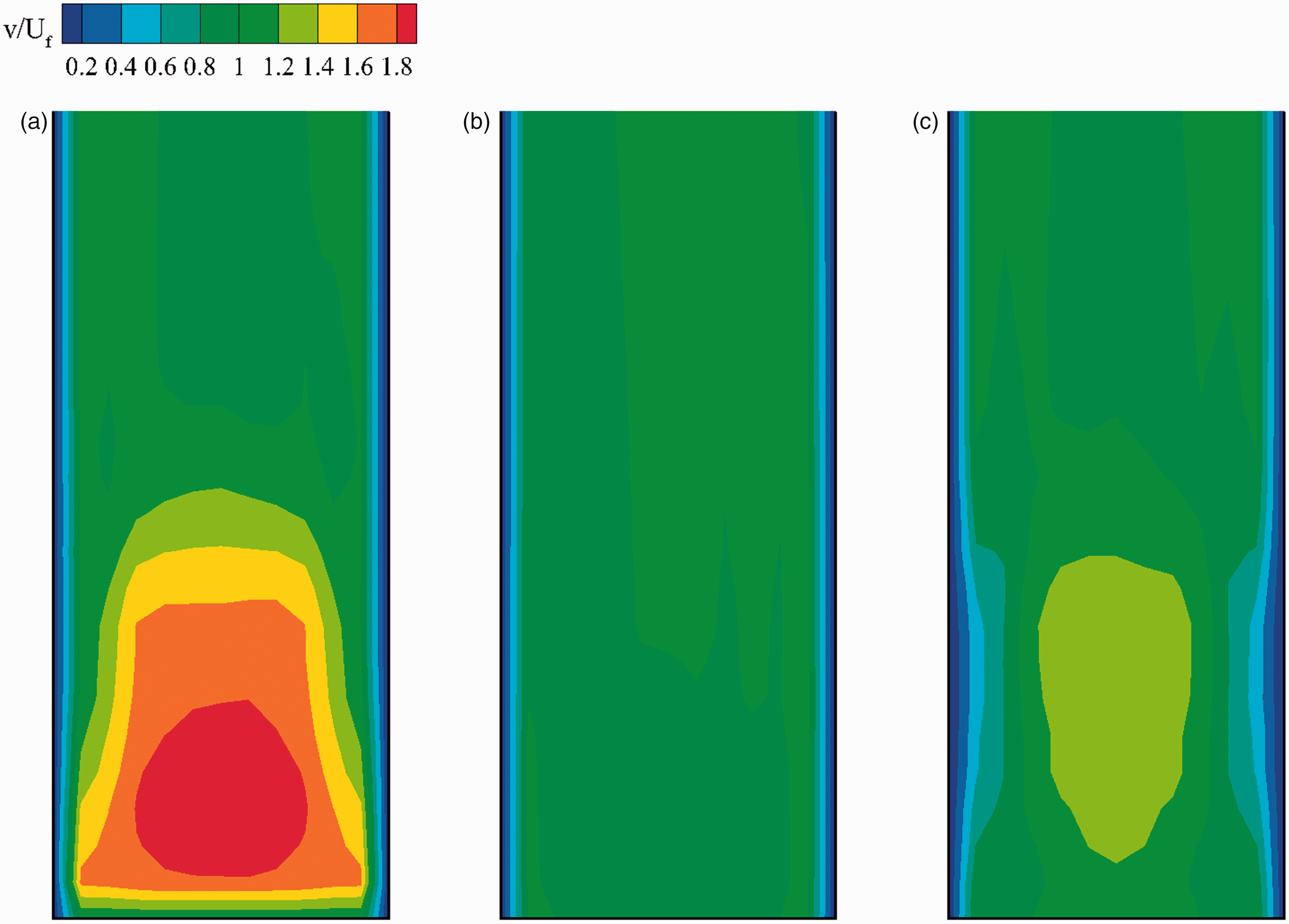
Comparison of averaged interstitial fluid velocity for (a) fully coupled simulation, (b) base partial coupling, and (c) revised partial coupling.
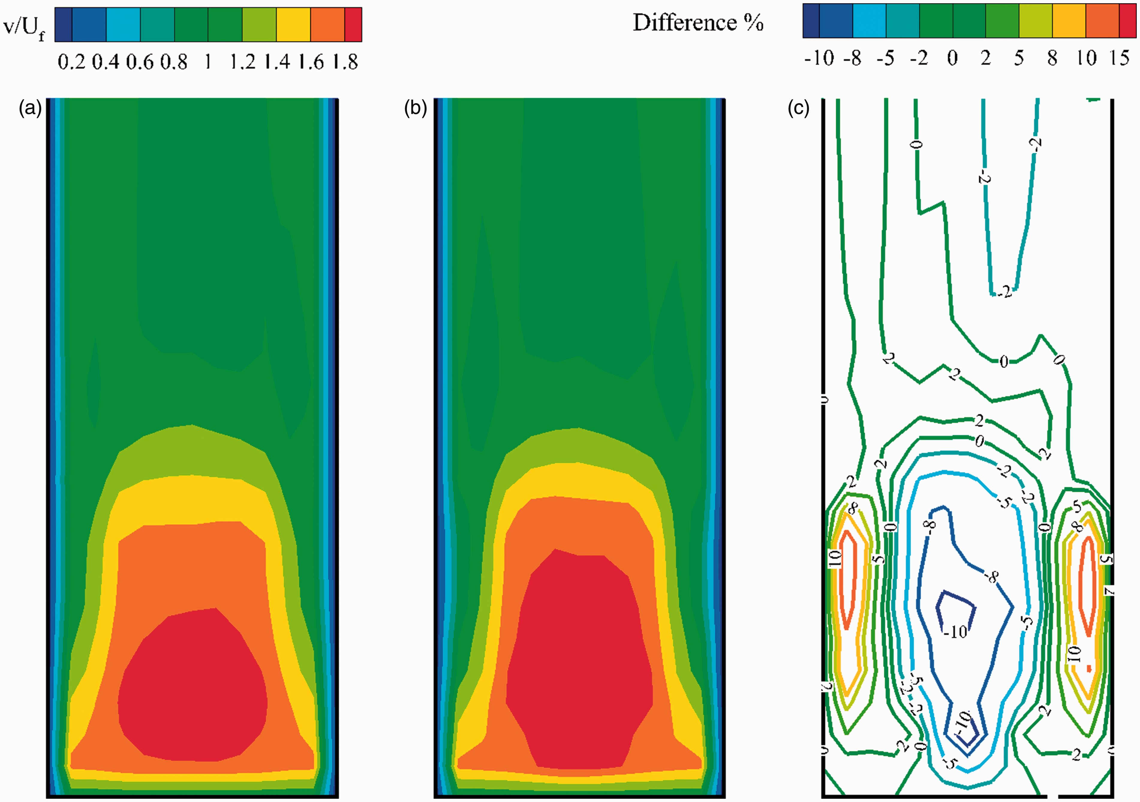
Comparison of averaged interstitial fluid velocity for (a) fully coupled simulation, (b) averaged projected interstitial velocity of the revised partial coupling, and (c) the difference between the two.
A comparison of the pressure signal at the last ∼5 s of the simulations is provided in Figure 6. The signal represents the difference between two probes: one is located at the bottom wall and the second is located at the top boundary (both adjacent to the side wall). The base partial coupling does not show pressure fluctuations because the bed is not bubbling. Both the full coupling and the revised partial coupling show good comparison of the instantaneous pressure drop signal. The mean pressure drops from the full coupling and the revised partial coupling are found to be 183.8 and 184.3 Pa. The difference between the two is ∼0.3%. Both mean pressure drops are slightly less than the weight of the bed of the particles (∼186.4 Pa). The mean pressure drop from the base partial coupling is found to be ∼174 Pa which is ∼5.5% less than the mean pressure from the full-coupling results. Interestingly, this small difference in pressure drop results in significant deviation in results. The rms value of the pressure drop signal for the full coupling and the revised partial coupling is found to be ∼36.3 and 23.6, respectively, with a difference of 10.1% between the two.
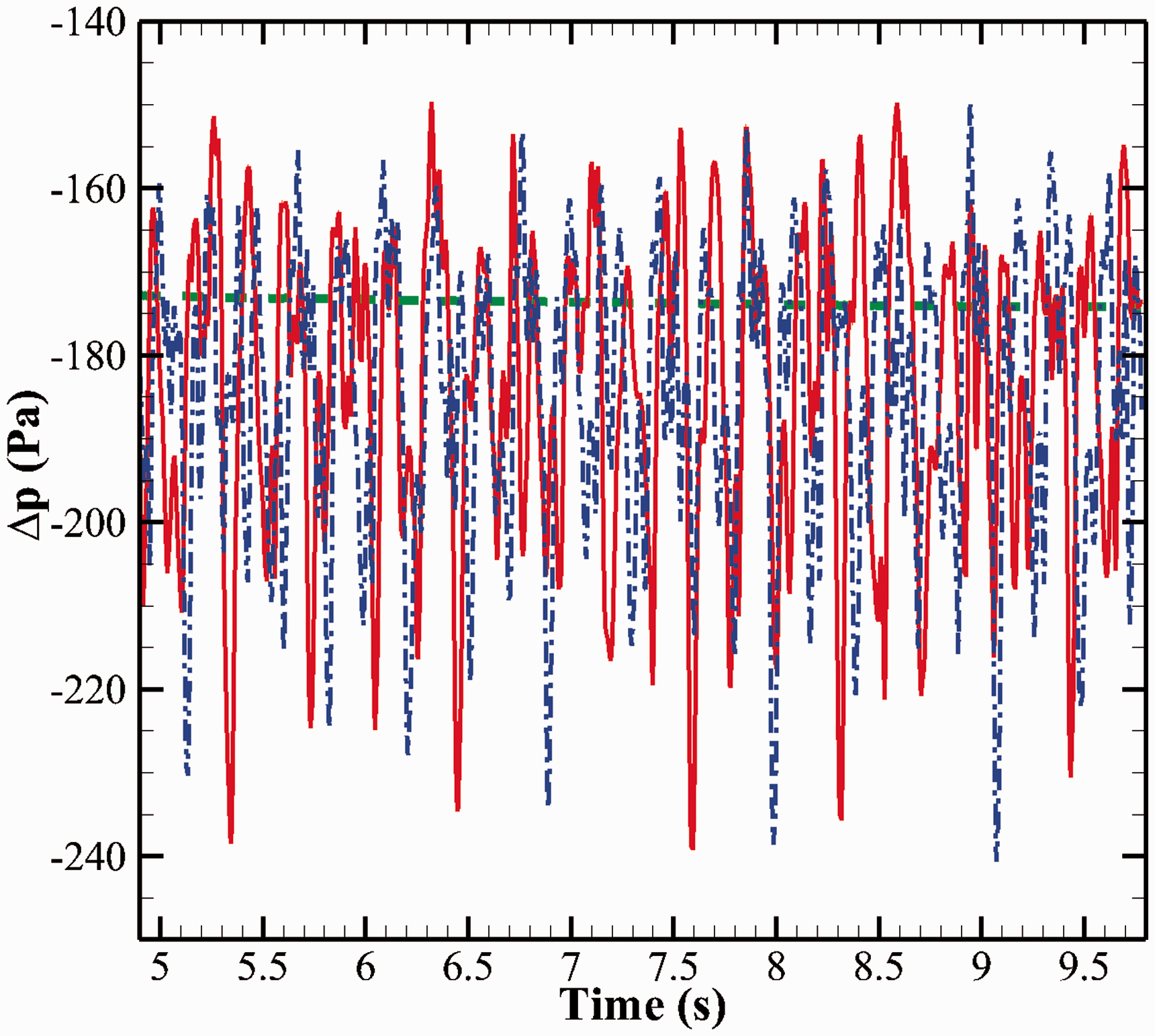
Pressure drop signal of the bubbling fluidized bed at the last 5 s of simulations using different coupling methods.
Sediment transport in turbulent open channel
A unidirectional turbulent open channel flow simulation used by Schmeeckle 29 is selected for the investigation of the performance of the different coupling techniques. All the simulations were run in a domain of 0.12 m × 0.06 m × 0.04 m divided into 120, 60, 65 cells in the stream-wise (x), cross-stream (z), and vertical direction (y), respectively. The grid is uniformly spaced in both stream-wise and span-wise directions. The vertical spacing is 0.2 mm in size for the first 20 grid cells above the bottom wall which is then gradually increased in size toward the top boundary. This particle bed height for bedload simulations (∼ 2 mm) is encompassed in the uniform grid region. The simulations comprised of O(105) mono-sized 0.5 mm spheres of density 2650 kg/m3 (medium sand) at different flow regimes. The properties of the particles used in the simulation are listed in Table 2. The simulations are performed in a turbulent open channel flow (Figure 7) with a velocity slip condition imposed on the top boundary and a no-slip condition on the bottom wall. The flow is periodic in both stream-wise and span-wise directions. The imposed mean pressure drop that balances the shear stress determines the value of the mass flow rate inside the channel. The fluid is water with a density of 1000 kg/m3 and a dynamic viscosity of 8.9 × 10⁻⁵ Pa s.
Numerical parameters of particles.
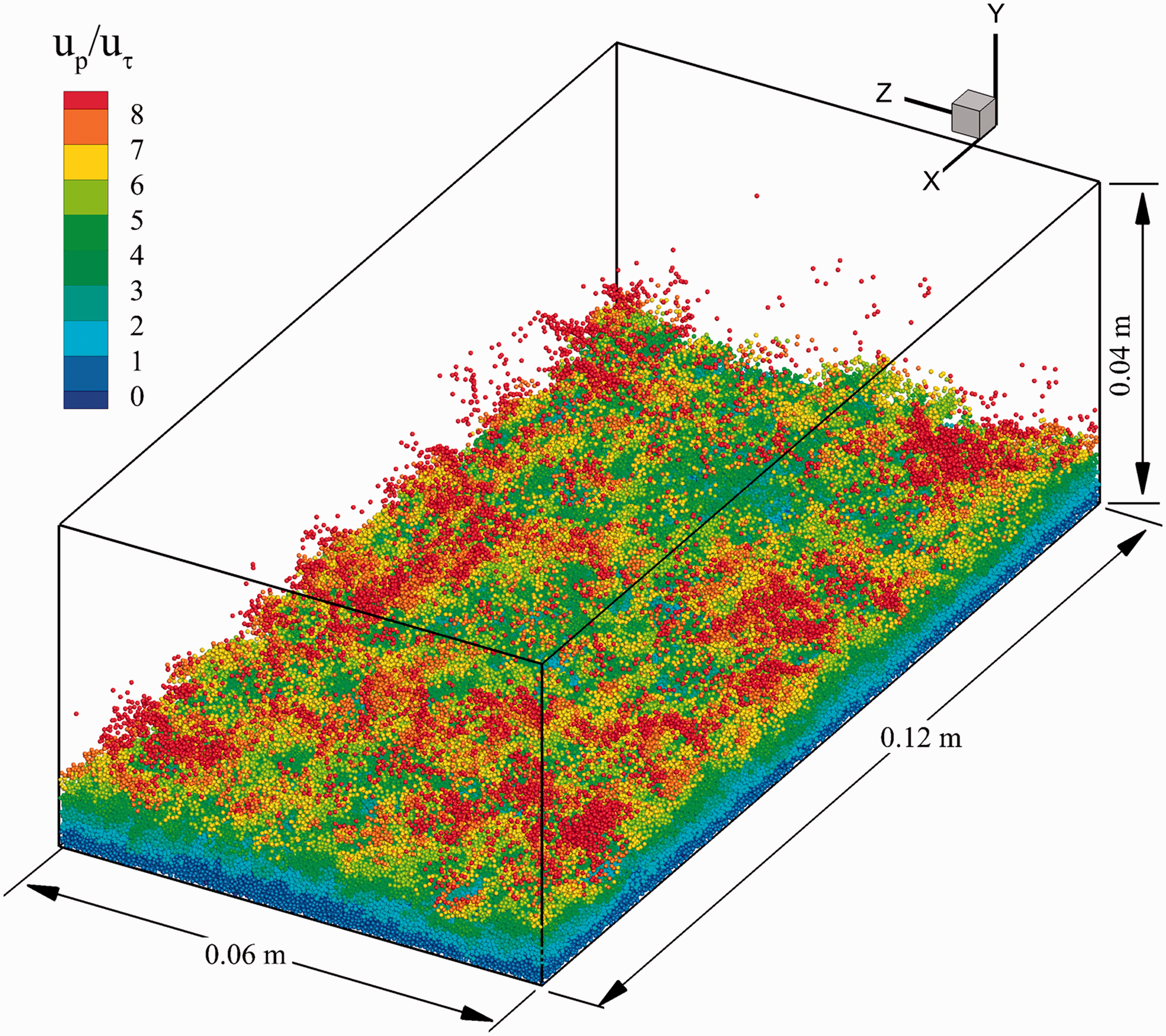
Calculation domain for the turbulent open channel flow.
Our previous work included 10 numerical experiments ranging from near incipience of motion of particles to strong suspension of particles.
33
At low flow rates or friction velocity, particle transport occurs in the bedload regime where particles move by rolling, sliding, and making small jumps over the bed (saltating). As the flow increases, particles get suspended in the flow by the action of turbulent structures and transport enters the suspended load regime. The transition from bedload to suspended load takes place roughly when the friction velocity (
In earlier work multiple numerical simulations of sediment transport in an open turbulent channel at flow regimes ranging from near incipience of particle motion to strong suspension were performed. The numerical experiments from using full coupling and base partial coupling showed good agreement in the bedload regime but underpredicted the sediment transport in the suspended load regime as compared to empirical formulas. 33 By moderately reducing the friction factor used in the numerical simulations good agreement was achieved in both bedload and suspended load regimes. 37 By comparing the base partial coupling predictions to the full-coupling approach it was found that the difference between the two was smaller in the bedload regime but became more obvious in the suspended load regime. 33 This was because in the bedload regime, most of the particles are static in the bed and the smaller drag force predicted by the partial coupling did not have a large impact, while in the suspended load regime many more particles are mobile and an underprediction of drag would have a much larger impact on overall particle transport.
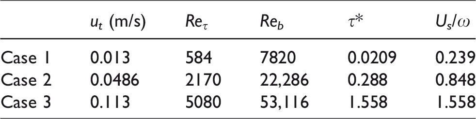
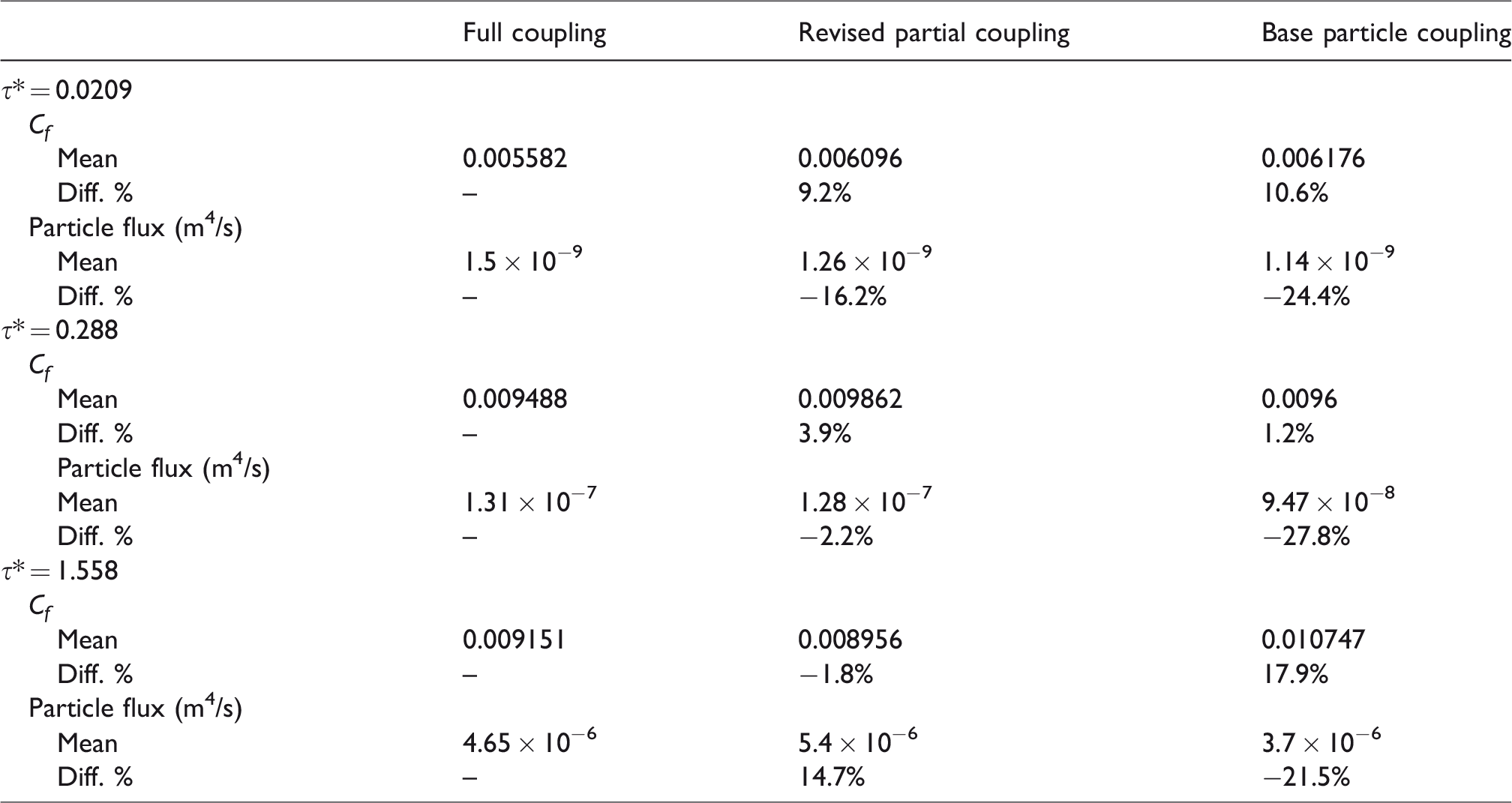
In the current work three simulations in different flow regimes are selected to investigate the impact of revised partial coupling on the simulations. The conditions of the selected simulations are presented in Table 3. The channel calculations were conducted using the revised particle coupling and compared to both a fully coupled formulation and a base partial coupling implementation in which the fluid velocity does not account for the presence of the solid. The simulations were run for 30 s of real time and the results are averaged in the last 10 s. Table 4 presents the quantitative values of the channel friction coefficient (Cf = (ut/ub)2 where ub is the bulk fluid velocity in the channel) and sediment transport or particle flux (the particle flux is the summation of the particle volume times the particle velocity) for the three cases along with the percentage error. The first case at a nondimensional shear stress of τ* ∼ 0.0209 represents a condition near the critical condition of particle movement. The second (τ* ∼ 0.288) and third (τ* ∼ 1.558) cases represent condition of high bedload and suspended load, respectively. As can be seen from the results in Table 4, the near incipience of motion and high bedload cases do not show significant change in the channel friction coefficient but the prediction of the particle flux improved noticeably. The improvement is more obvious for the high bedload calculation. The suspended load simulation, on the other hand, shows an improvement in both the predicted channel friction coefficient as well as sediment transport. Although the error in the predicted sediment transport is much smaller, it is overpredicted compared to the fully coupled case by about 15%. The temporal evolution of the mean channel friction and the sediment transport are presented in Figure 8(a) and (b), respectively, for the suspended load case of τ*= 1.558. Good agreement of the channel friction coefficient can be seen in Figure 8(a) where the particle flux is slightly overpredicted. The base partial coupling underpredicts the particle flux because effectively the superficial velocity is used in the drag correlation which gives a lower drag force on the particles, thus less number of particles are set in motion. With the revised partial coupling, the physically consistent interstitial velocity is used in the drag force calculation thus increasing the force on the particles and making them more mobile. This increases the particle flux. On the other hand, because less number of particles are set in motion with base partial coupling, they collectively resist the fluid motion more than the revised partial coupling, thus increasing the friction coefficient.
Simulation conditions for the selected cases.
Mean friction factor (Cf) and sediment transport for the three selected cases.
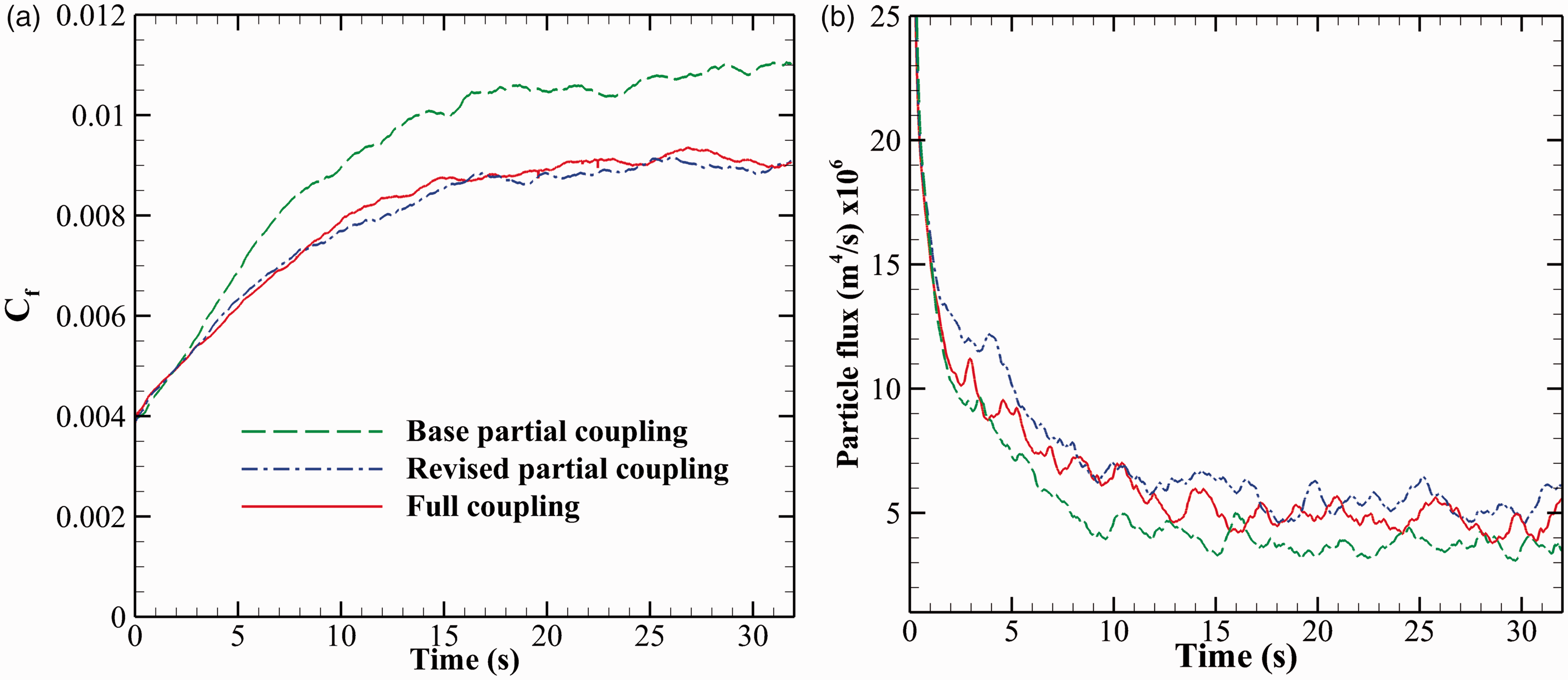
Temporal evolution of (a) friction coefficient (Cf) and (b) particle flux for case 3 (τ* ∼ 1.56).
Convergence and stability of calculations
As was mentioned earlier in the manuscript, the fully coupled method typically takes many more iterations in the pressure equation to reach convergence because of the inclusion of the void fraction in mass and momentum conservation. Figure 9 presents a comparison between the convergence behavior between a fully coupled simulation and revised partial coupling for 25 successive time steps under the same conditions. The interval between time steps is divided into 250 segments representing the maximum number of permissible iterations. The convergence criterion for the pressure equation at each time step is set to a strict value of 1 × 10⁻⁶. As can be seen from Figure 9, the revised partial coupling converges in roughly 20 iterations (each marker indicates five iterations) whereas the full coupling at most all time steps does not converge to a residual of 1 × 10⁻⁶ in the allotted 250 iterations and diverges at the 25th time step. In fact, increasing the maximum number of permissible iterations at each time step not only increases computational complexity but also makes the solution unstable earlier.
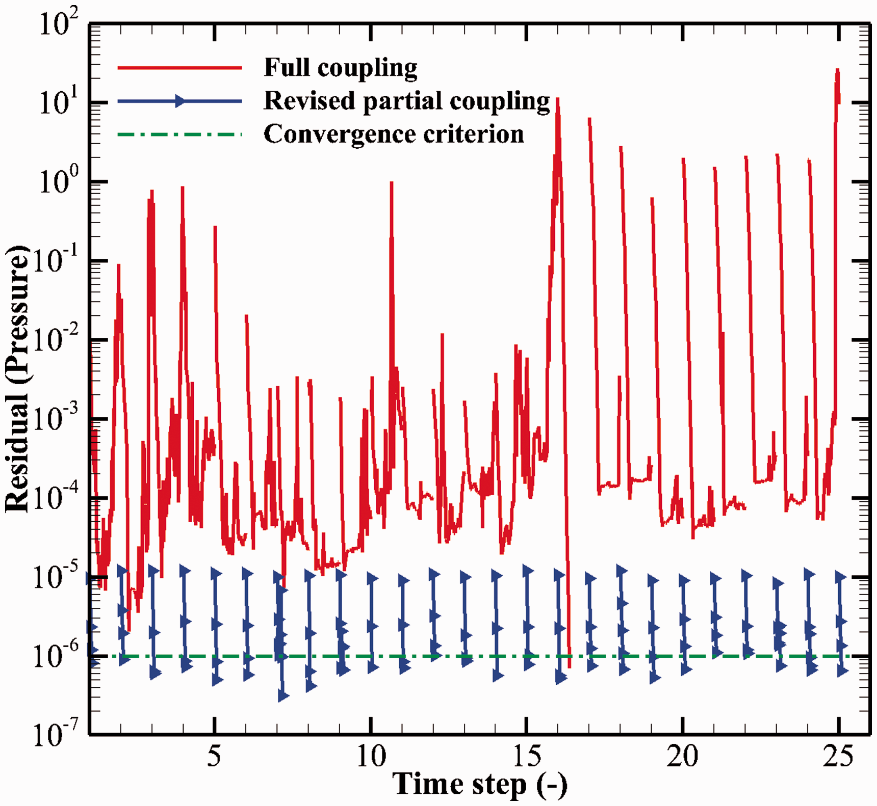
Sample of convergence for successive 25 time steps for the sediment transport simulation (τ* ∼ 1.56) for a strict convergence criterion using full coupling and revised partial coupling.
Speedup of calculations
A summary of the performance outcome of all the conducted simulations is presented in Table 5. Since the fluid grid in the fluidized bed simulation is very coarse, the time spent in the fluid part of the calculation is quite small and while improvement in the convergence is evident, the overall impact is minimal. The base partial coupling for the bubbling fluidized bed takes longer time to run because the resultant static bed results in more collisions that need to be processed. For the sediment transport simulations, the fluid solution time increases from bedload to suspended flow ranging from 25 to 35% for the fully coupled solution. In contrast, the revised partial coupling varies between 14 and 21% of the total solution time. For these set of calculations with 10 particle substeps for each fluid time step, the savings in total run time using partial coupling are modest ranging from factors of 1.07 to 1.53 with savings in fluid solution time ranging from factors of 1.35 to 4.35. It is projected that for particle transport in high Reynolds number turbulent flows, the savings would be more substantial. The speedup reported in the sediment transport simulations is obtained when the maximum number of pressure iterations is limited to 100. It is emphasized here that the revised partial coupling be used in cases where full coupling is not feasible rather of considering it as a less expensive alternative.
Averaged performance for 2.5 s of real time for all considered simulations.
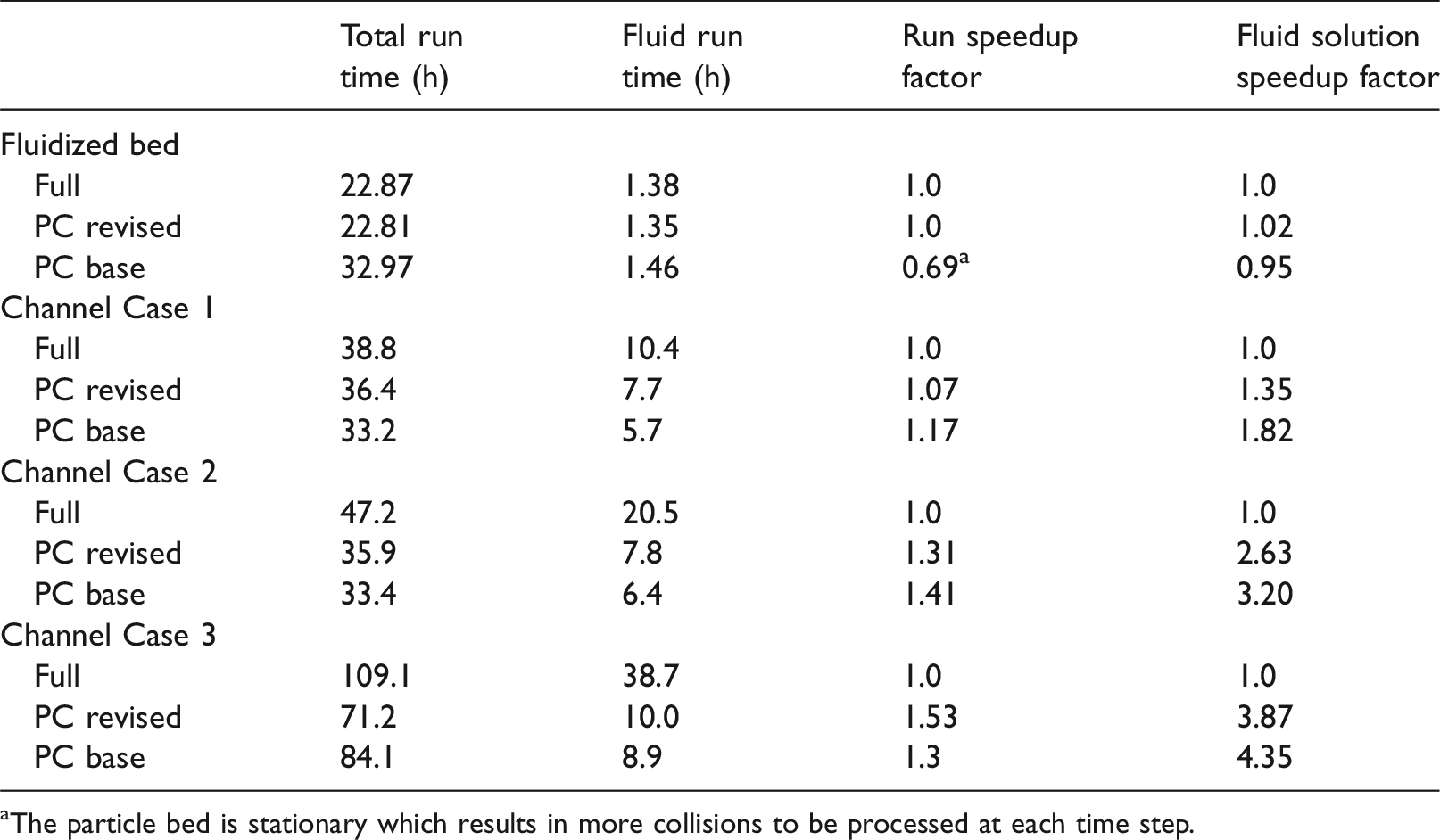
aThe particle bed is stationary which results in more collisions to be processed at each time step.
Conclusions
In this work a revised partial coupling formulation is proposed for use with dense particulate flow systems that show hard convergence behavior. The revised coupling assumes a void fraction of unity in the solution of fluid momentum equations but modifies the relative velocity used in point mass force models to compensate for this omission. Omitting the spatiotemporal variation of void fraction in the momentum equations results in much faster convergence and enhances the numerical stability. Including a modified interstitial relative velocity in point mass force calculations, on the other hand, compensates for the lower fluid velocities calculated by the momentum equations. Without this correction, it was found that particle mobility was underpredicted when using partial coupling. The efficacy of the revised partial coupling is demonstrated in two different fluid–particle systems consisting of a bubbling fluidized bed and turbulent sediment transport. In both systems, it is shown that the proposed method shows much better comparison to the fully coupled approach. In the fluidized bed experiment, without the proposed modification, the bed does not fluidize in spite of a fluidization velocity which is three times the minimum fluidization velocity. In turbulent sediment transport, the improvement in predictions is more subtle. In the bedload regime in which particles are not very mobile, the improvements are slight, but as the flow becomes more energetic entraining more particles into suspension, the proposed modification progressively shows more improvement over the base partial coupling.
Using the partial coupling, the fluid solution time was found to be reduced by factors ranging from 1.35 to 4.35. The reduction in the fluid solution is more significant for simulations that are difficult to converge and those in which the fluid calculation takes a considerable percentage of the overall simulation time. Fully coupled simulations that exhibit difficult convergence behavior or those which diverge due to numerical instabilities can benefit the most from using this technique. The revised partial coupling is not recommended as a substitute for full coupling but as an alternative method when full coupling gives rise to numerical difficulties, particularly in problems involving combustion of particles.
Footnotes
Acknowledgments
Husam Elghannay would like to express his sincere thanks to the Higher Libyan Ministry of Education and Scientific Research for the scholarship opportunity to pursue his PhD study at Virginia Tech. The authors would also like to extend their gratitude to the Mechanical Engineering Department at Virginia Tech for granting a Hord fellowship to Mr Elghannay. The authors are also grateful to Virginia Tech Advanced Research and Computing for providing access to computational resources for this work.
Declaration of conflicting interests
The author(s) declared no potential conflicts of interest with respect to the research, authorship, and/or publication of this article.
Funding
The author(s) disclosed receipt of the following financial support for the research, authorship, and/or publication of this article: The article proecssing charges were funded by Virginia Tech's Open Access Subvention Fund.