Sage Journals: Discover world-class research

Abstract

The transient performances of impeller machinery under typical mutational working conditions play an important role in the area of engineering and have attracted extensive attention. In order to fully understand transient behaviors of impeller machinery under mutational working conditions, it is very necessary to confirm an efficient and reliable solving method. In this paper, the dynamic mesh method and the sliding mesh method are respectively used to be solved the inner transient flow of a 2D centrifugal pump model during abrupt start-up period. The Renormalization-group (RNG) k–ε turbulence model in eddy viscosity models is chosen to close the Reynolds-average equation and to complete the turbulence calculation. Moreover, the SIMPLE algorithm is also adapted to accomplish the coupling calculation between velocity and pressure. The study shows that in theory, the most appropriate method to solve transient flow is the dynamic mesh method, but it has the shortage of low mesh quality during mesh reconstruction. The sliding mesh method with high mesh quality is an ideal solving method under mutational working conditions. In general, both of the methods would reflect the basic characteristics of inner flow, while the sliding mesh method has higher solution precision.

Keywords

Impeller machinery centrifugal pump mutational working condition dynamic mesh sliding mesh

Introduction

Impeller machinery including vane pump, hydro turbine, wind turbine, and compressor, etc. have been widely used in industry and agriculture, which are regarded as an essential transport device for fluid media. Since the invention of impeller machinery, scholars at home and abroad made in-depth and detailed studies to improve its overall performance. However, almost all the researches are carried out under steady working conditions,^1–4 while there are few studies on performance of impeller machinery under mutational working condition, such as abrupt start-up, power outage, and rapidly regulating discharge valve opening, etc. Meanwhile, the transient processes that often cause equipment failure exist inevitably. Therefore, it is very necessary to carry out the study on transient behaviors so as to fully understand the performance of impeller machinery under mutational working condition, as well as meet the increasing requirement of modern engineering.

Under mutational working conditions, for example, starting, stopping, regulating discharge valve, and fluctuating rotation speed, some flow parameters would be changed drastically in a very short period. For example, during start-up of the pump, physical parameters (rotation speed, flow rate, pressure, etc.) increase sharply, and the Reynolds number increases from zero to millions, which could be even 10 million in some cases. The flow regime changes from laminar flow to turbulent flow, turbulence intensity varies rapidly as well as shear stress. This flow inside the pump belongs to typical rapidly varied flow, namely unsteady flow with rapid variation or transient flow. The performance of impeller machinery is determined by the characteristics of flow field. The rapid development of computational fluid dynamics provides a convenient method to solve internal fluid field, and has become a mainstream research method. In order to precisely obtain the characteristics of fluid field, it is very necessary to use a high-efficient and reliable numerical method. This paper focuses on the numerical simulation for the quick start-up process of a low-specific speed centrifugal pump by means of the dynamic mesh method⁵ and sliding mesh method,⁶ respectively. In Wang et al.,⁵ the entire computational region was described using the absolute reference coordinate system, with the dynamic mesh method dealing with the moving boundary caused by the accelerating pump blade. In Wu et al.,⁶ the flow domain was divided into two regions: dynamic and stationary. The dynamic region is accelerated as an entirety whose rotational speed is assigned with a given function here. Each region was independently discretized and then the regions with shearing boundaries are dealt with non-conformal grids at grid interfaces.

Through analyzing the varying grids and flow fields during start-up period, it could conclude the optimal numerical solution method for mutational working conditions. At the end of this paper, aiming at four typical mutational working conditions, the numerical solution strategies, which point out the direction for further calculations would be put forward in detailed.

Computational model

As an example, the two-dimensional (2D) model of a centrifugal pump is chosen as a computational model, shown in Figure 1. The outlet width of volute model is 40 mm, the impeller diameter is 160 mm and the blade number is 6, the blade profile is 2D-cylindrical, the blade thickness is 3 mm and the blade angle at inlet and outlet are 25°, respectively. This emphasis of this paper focuses on the feasibility and merits of alternative computational methods for mutational working conditions, taking no account of the varying characteristics of flow inside pump model. To facilitate calculation, assume that the inlet and the outlet of pump model are both solid surfaces as well as blades.

Figure 1.

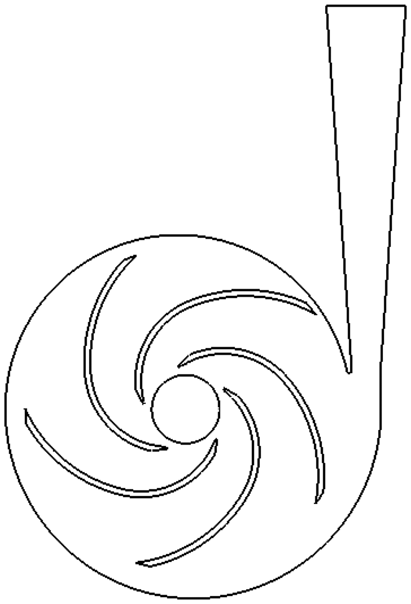
2D model of a centrifugal pump.

Assume that the rotation speed of the blades is increasing regularly according to the following rule.⁷

N (t) = N_{0} \exp (1 - t / T_{n d})

(1)

where N₀ is 1450 r/min, T_nd is nominal acceleration time, 0.15 s in this paper.

In the process of impeller acceleration, the change rule of rotating speed is uploaded to FLUENT by programming user-defined function (UDF) according to the equation (1). The calculation selects RNG k–ε turbulence model in eddy viscosity models, which is verified to high efficiency simulate the flow with high revolution rate and curvature.⁸ Considering viscosity, the no-slip boundary condition is applied on wall surface. Meanwhile, the standard wall function is used to solve the flow near walls when the turbulence model with high-Reynolds number is applied. The time discretization of transient term adopts first-order implicit scheme. The spatial discretization of convection term, diffusion term, and source term uses second-order upwind scheme, second-order accurate central difference scheme, and linearized standard format, respectively. The coupling of velocity and pressure is achieved by SIMPLE algorithm. Variables in iteration are determined by default under-relaxation factors in FLUENT software. The value of time step is set as 0.0001 s according to our calculation experience and the total start-up time is 1.0 s. Set the maximum number of iteration as 100 times in each time step, to ensure the absolute convergence. The constringency residuals of all solved parameters are set as 0.0001.

Numerical method

In this paper, two methods (dynamic mesh method and sliding mesh method) would be used to solve the internal instantaneous flow fields of a physical pump model during starting periods. The difference between two results obtained through two methods could be found.

Dynamic mesh method

Dynamic mesh method could be used to simulate the internal flow that is caused by boundary movement through the boundary-type function or UDF. The numerical computation in this paper is completed by using FLUENT software. 2D numerical computation of pump model adopts the elastic coefficient algorithm and the local reconstruction algorithm in dynamic mesh method to reconstruct the grids during acceleration period. In elastic coefficient algorithm, the edge between any two arbitrary grid nodes is equivalent to a spring. The UDF defined by user firstly computes the displacement of nodes on boundary. This displacement produces an elastic force whose magnitude is proportional to that of displacement on an arbitrary edge connected to the node. Thus, the displacement on boundary node is transferred to the whole meshes. In balance state, the sum of the elastic force on edges connected to the node is zero. The balance generates a cyclic formula for node displacement:

Δ {\vec{x}}_{i}^{m + 1} = \frac{\sum_{j}^{n_{i}} k_{i j} {\vec{x}}_{j}^{m}}{\sum_{j}^{n_{i}} k_{i j}}

(2)

where Δx_i is the displacement of node i, n_i is node number connected to node i, k_ij is the elastic constant between node i, and adjacent node j, which is defined as:

k_{i j} = \frac{1}{\sqrt{| {\vec{x}}_{i} - {\vec{x}}_{j} |}}

(3)

When the displacement of boundary node is known, Jacobian scanning algorithm could be used to solve the above formula. The position of inner node is updated after obtaining the convergent solution.

{\vec{x}}_{i}^{n + 1} = {\vec{x}}_{i}^{n} + {\vec{x}}_{i}^{k, converged}

(4)

where n + 1 and n represent the next and present time step, respectively.

Variation of mesh

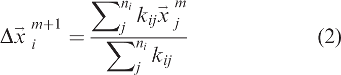
The total mesh numbers before deformation are 94,398. Results show that when the starting time are respectively 0.005 s, 0.020 s, 0.035 s, and 0.50 s, the total mesh numbers after deformation are 94,012, 90,254, 75,183, and 45,971, respectively. As we know, such a number may not be sufficient to identify small-scale structure of boundary layers, but may predict the performance and capture the large-scale flow phenomenon correctly. Moreover “EquiAngle Skew” and “EquiSize Skew” of all meshes are less than 0.85. For wall y+, the values at four starting moments are respectively about 30, 60, 100, and 210 near the boundary wall. Therefore, the grid quality is severely deteriorated.

For present mesh number and computation setting, calculations are parallelly performed on a Windows PC cluster of four Intel Xeon processors (3.2 GHz). The simulation of the startup requires approximately 10 days.

In the process of start-up, the deformation and evolution of 2D meshes inside centrifugal pump based on dynamic mesh method are shown in Figure 2. It is observed that when starting time t = 0.005 s, instantaneous rotation speed n = 47.5 r/min, the rotation speed is quite low, and the meshes inside centrifugal pump have not be deformed and reconstructed significantly. When starting time t = 0.020 s, instantaneous rotation speed n = 181 r/min, the rotation speed rises sharply. In addition, the meshes inside centrifugal pump, especially near rotating blades, show obvious deformation and reconstruction. The blades counterclockwise rotate in present calculations, which show that the mesh reconstruction near pressure sides of blades is relatively well, as well as relatively small grid deformation. However, the grid deformation on suction sides of blades is relatively serious, the quality of mesh reconstruction reduces significantly, the size of maximum mesh is oversize, and large grids take most area of blade channels. When starting time t = 0.035 s, instantaneous rotation speed n = 302 r/min, it can be seen that the grids near blade pressure sides still keep good quality. Meanwhile, the grid deformation near blade suction sides is very serious, namely that the grid reconstruction quality is greatly reduced. It is also seen from Figure 2 that the size of the largest grid is very high, which occupies most of the impeller passage area. When starting time t = 0.050 s, instantaneous rotation speed n = 411 r/min, the meshes near pressure sides and suction sides of blades are with relatively good quality. However, besides the poor quality of mesh inside blade channels, the mesh deformation is serious as well as the size proportion between large and small meshes. Anyhow, to calculate the inner flow under mutational working conditions by using the dynamic mesh method, the inner meshes are deformed seriously. In other words, the mesh quality is very poor.

Figure 2.

Variation of mesh based on dynamic mesh method. (a) 0.005 s; (b) 0.020 s; (c) 0.035 s; and (d) 0.050 s.

Variation of dynamic pressure

Based on the dynamic mesh method, the evolution of dynamic pressure inside 2D centrifugal pump during start-up is shown in Figure 3. When starting time t = 0.005 s, instantaneous rotation speed n = 47.5 r/min, it is seen from Figure 3(a) that the average dynamic pressure is quite low and uniformly distributed, which could attribute this fact that the relatively low rotation speed results in the relatively low internal flow, the low internal flow velocity results in the low dynamic energy. As a result, the average dynamic pressure is only about 0.5 kPa. When starting time t = 0.020 s, instantaneous rotation speed n = 181 r/min, with significant increasing of rotation speed from 47.5 r/min to 181 r/min, it is obvious from Figure 3(b) that the distribution of the dynamic pressure inside impeller channels begins to become uneven, which indicates that the flow velocity magnitude in different regions shows differences. Clearly, the inner backflow inside 2D pump model under low flow rate condition is the main reason for differences in dynamic pressures. When starting time t = 0.035 s, instantaneous rotation speed n = 302 r/min, it is observed from Figure 3(c) that the dynamic pressure on blade pressure sides is obviously higher than that on blade suction sides. When starting time t = 0.050 s, instantaneous rotation speed n = 411 r/min, the overall value of average dynamic pressures has a significant rise, especially in the middle section of blade pressure sides, which could attribute to the increase through velocity inside impeller channels with the growth of rotation speed.

Figure 3.

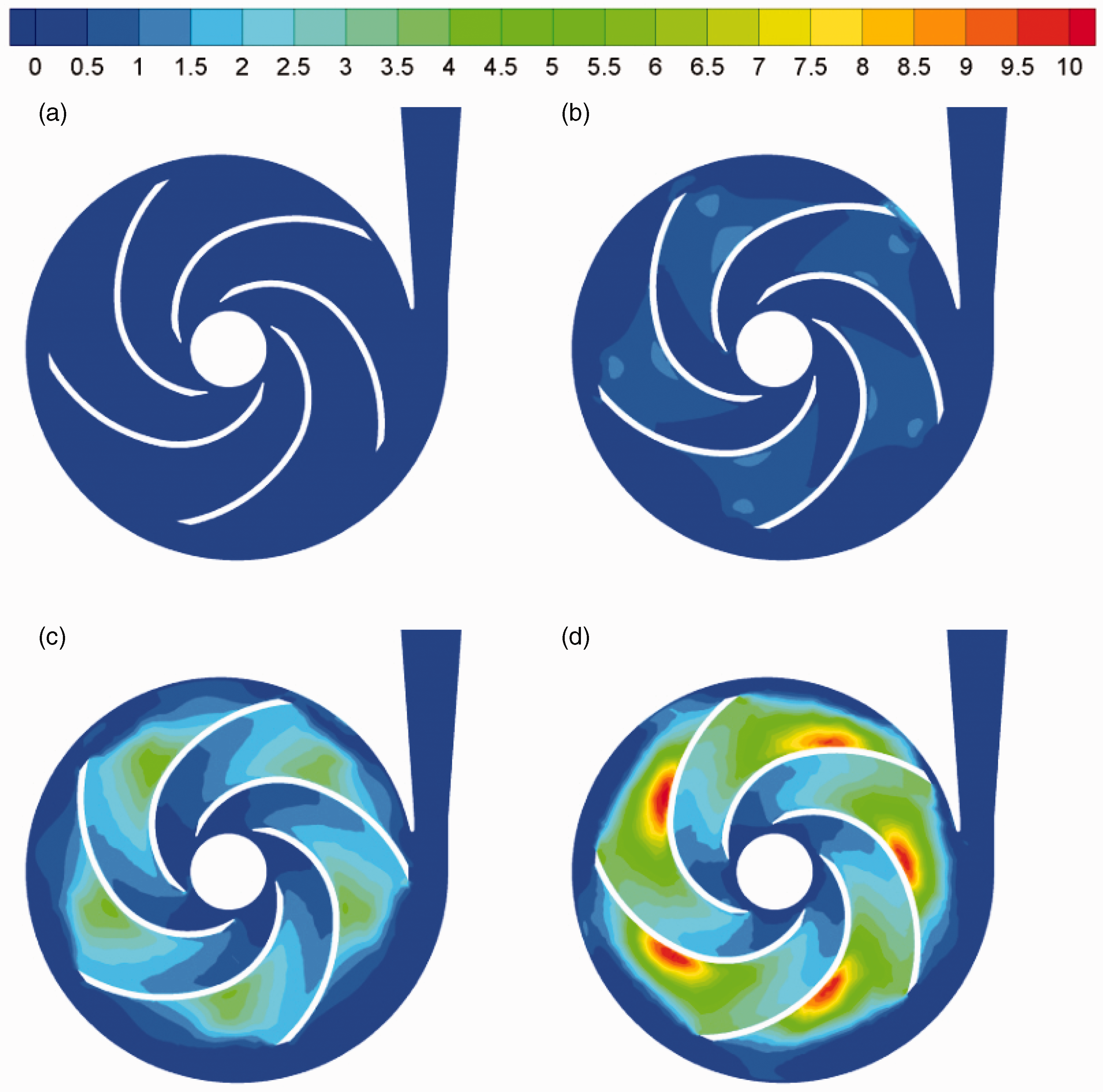
Variation of dynamic pressure based on dynamic mesh method. (a) 0.005 s; (b) 0.020 s; (c) 0.035 s; and (d) 0.050 s.

Sliding mesh method

When using the sliding mesh method to calculate the flow, the grids on either side of the interface slide against each other with the same flux on both sides rather than coincide with each other. The sliding meshes transfer data through interface without mesh reconstruction. After iteration in each time step, the overall sliding region moves as specified, and then the iteration in next time step.

Variation of mesh

The total mesh numbers in sliding mesh method are always 94,548. Likely, these meshes are also insufficient to capture micro flow structure, for example in boundary layers, but are also able to be used to predict the macroscopical performance and capture the macroscopical flow phenomenon. Meanwhile, the grid quality is also satisfied, the “EquiAngle Skew” and “EquiSize Skew” of all meshes are also less than 0.85. Likely, the simulation of the startup requires also approximately 10 days, which could be attributed to the fact that the mesh numbers between them are almost the same.

When start-up, the variation of 2D centrifugal pump’s inner mesh based on the sliding mesh method is shown in Figure 4. When starting time t = 0.005 s, 0.010 s, 0.015 s, and 0.020 s, the corresponding rotation speeds are 47.5 r/min, 93.5 r/min, 138 r/min, and 181 r/min, respectively. It is observed that the grids waiting for computing keeps completely the same as the initial construction with no change, namely that the grids are not deformed. In other words, the mesh retains very good quality without any variation.

Figure 4.

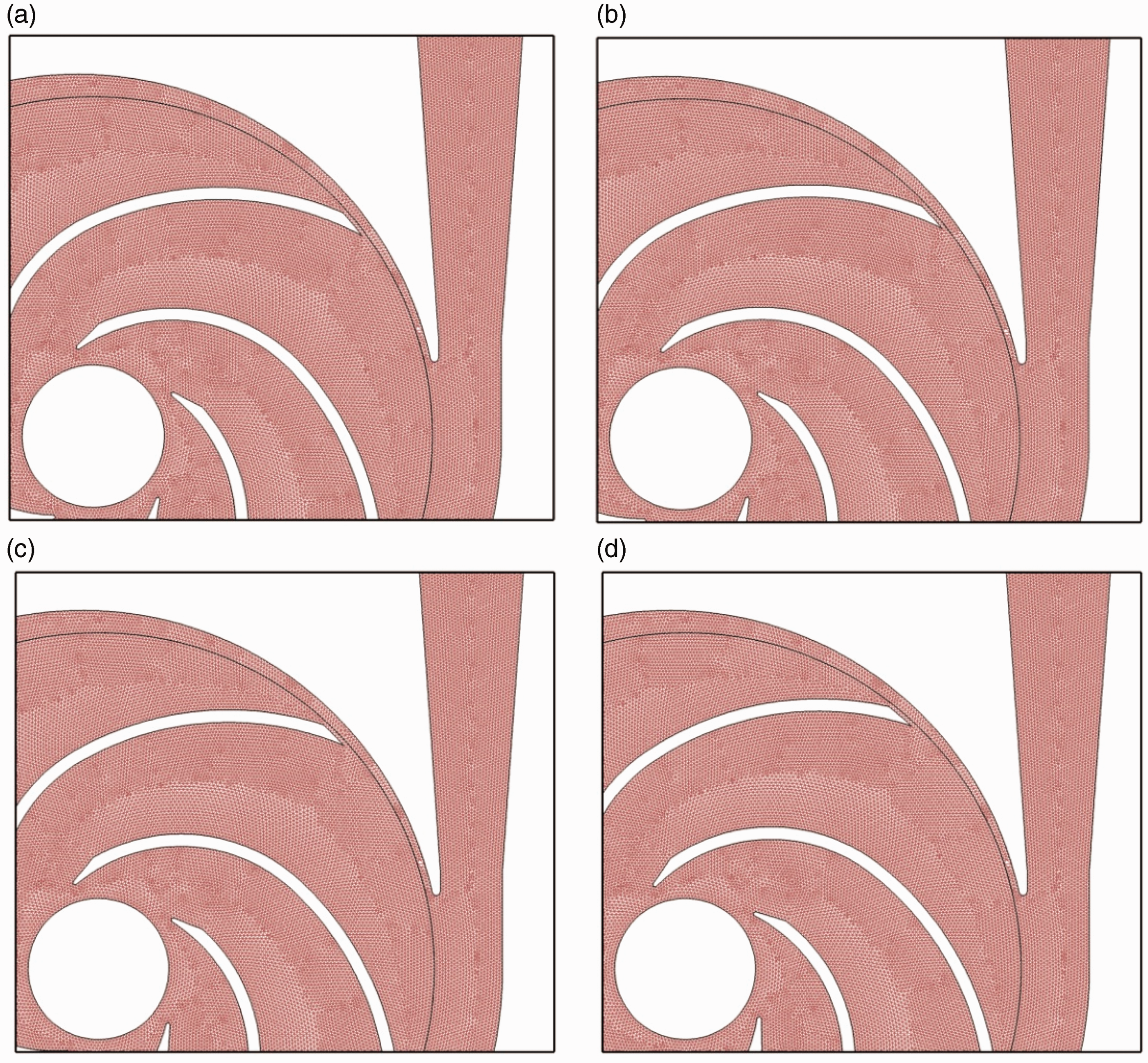
Variation of mesh based on sliding mesh method. (a) 0.005 s; (b) 0.010 s; (c) 0.015 s; and (d) 0.020 s.

Variation of dynamic pressure

The evolutionary history of the dynamic pressure inside 2D centrifugal pump based on sliding mesh method during start-up is shown in Figure 5. When starting time t = 0.005 s, instantaneous rotation speed n = 47.5 r/min, the rotation speed is relatively low, and the dynamic pressure distributes uniformly. However, there are some local high pressures at outlet of the blade near volute tongue, which is different from the low-pressure features in dynamic mesh method. When starting time t = 0.010 s, Figure 5(b) shows that it has good symmetrical characteristics with tallish pressure at the middle of pressure sides and the outlet of the blades, while for other area, the dynamic pressure is distributed uniformly and keeps relatively low values. When starting time t = 0.015 s and 0.020 s, the distributions of the dynamic pressure present typical characteristics and symmetry with the increasing rotation speed.

Figure 5.

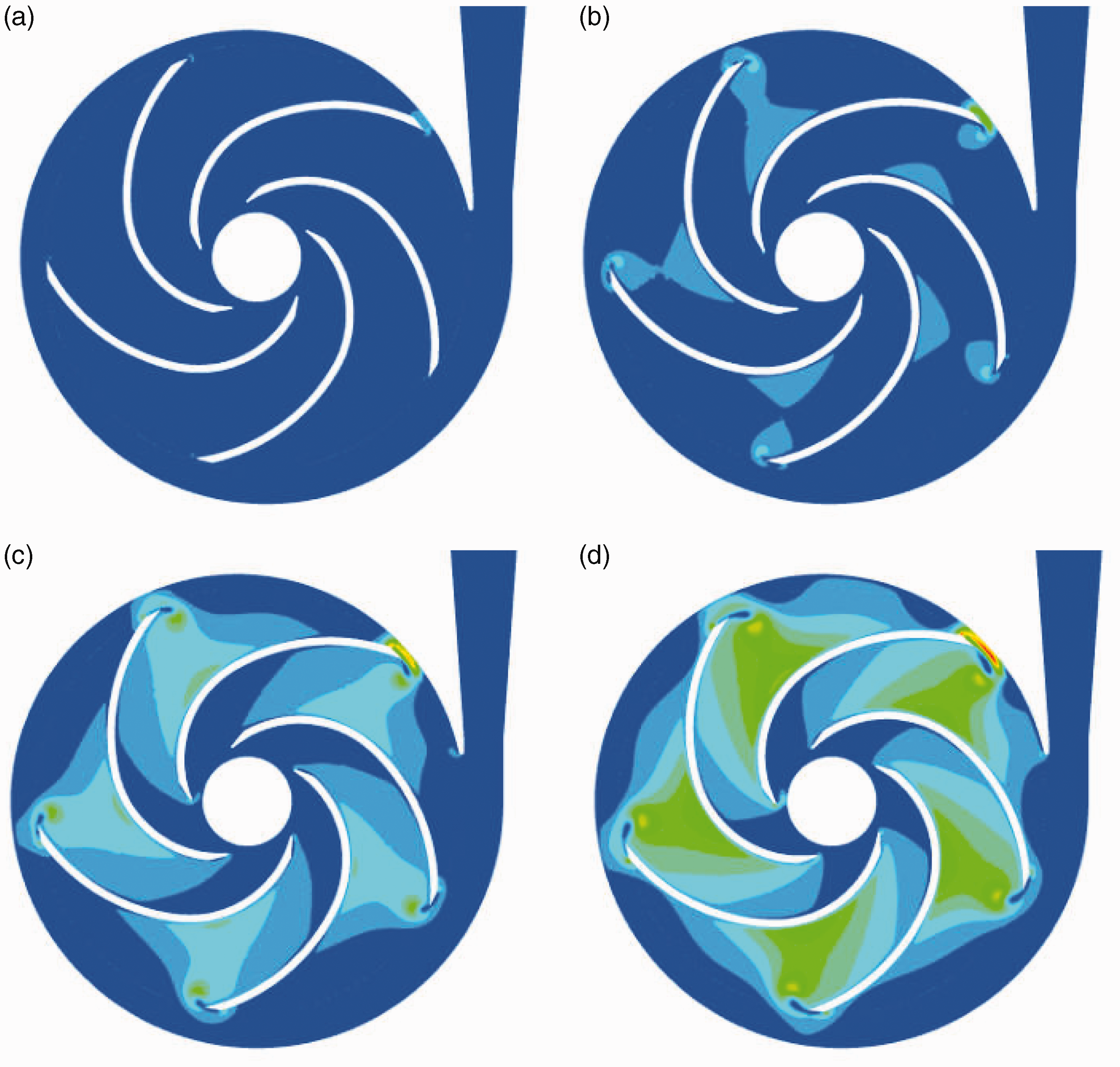
Variation of dynamic pressure based on sliding mesh method. (a) 0.005 s; (b) 0.010 s; (c) 0.015 s; and (d) 0.020 s.

Solution strategy on mutational working conditions

The mutational working conditions of centrifugal pumps include abrupt start-up, power outage, quick adjustment of discharge valve (alternative working condition), and instantaneous fluctuation of rotation speed. For numerical computation of unsteady flow under four mutational working conditions, the accurate specifications of boundary conditions are the key problem. Therefore, the solution strategies, namely two calculation methods for a single isolated pump⁹ and the circulating pipe system including pump,^10,11 are established as follows.

Single pump

Start-up

In the process of pump’s start-up, the rotation speed-up of impeller is mainly determined by the driving equipment (e.g., motor). Usually, the experimental results of the rotation speeds during start-up period are regarded as one of calculation conditions in the process of numerical simulation. At the inlet and outlet of pump model, the variation rules of the pressure or the flow rate based on experimental results are usually regarded as the corresponding boundary conditions in numerical calculation. In order to avoid power overload phenomenon, centrifugal pumps are usually required to start up in the case of closing the discharge valve. For this case, there is no need to give the change rules of performance parameters at the inlet and outlet of pump model in numerical calculation.

b. Power outage

In the process of power outage, the driving equipment, for example, motor, no more provide any driving torque to the rotating impeller. For this case, the drag torque of moving fluid media acting on impeller is the main reason for degradation of blade’s rotation speed. Therefore, the inner transient unsteady flow could be solved by given variation rule of the rotation speed. Otherwise, iterate stable torque calculated from steady rotation speed before stopping could be used to solve rotation speed of pump. At the inlet and the outlet of pump model, the setting of boundary conditions is the same as that during start-up period.

c. Regulating discharge valve

In the process of regulating discharge valve, the rotation speed is usually considered to be constant. As a result, rapid adjustment of discharge valve is actually changing the magnitude of flow rate, namely variable working conditions. Therefore, at the inlet of pump model, the variation rule of the flow rate is the only boundary condition needed to be given. Meanwhile, at the outlet, it could only specify as free flow condition.

d. Fluctuation of rotation speed

In the process of fluctuating rotation speed, it fluctuates with flow time. Therefore, the flow parameters at the inlet and the outlet of pump model would change correspondingly. Besides the given fluctuation rule of the rotation speed in calculation, the experimental results of the flow rate or pressures at the inlet and outlet of pump model need to be specified as the corresponding boundary conditions.

Overall circulation pipe system

When the calculation domain is the overall circulation pipe system including pump model, water tank, discharge valve, and pipes, etc., there is no need to give the boundary condition at the inlet and outlet of pump model. (1) For start-up and fluctuating rotation speed, it is only required to give the variation rule of rotation speed according to experimental result. (2) For power outage, the given drop rule in rotation speed or the iterative computation of the hydraulic torque of fluid media acting on impeller is enough for calculation. (3) For varying working conditions, the corresponding calculation can be accomplished by regulating the discharge valve.

Discussion

In this paper, we emphatically analyze the feasibility of two solving methods to calculate the internal transient flow insides 2D pump model. In future works, we would analyze and assess the prediction accuracy of two methods by means of experimental results of transient performance.

Conclusions

This paper based on an example of 2D centrifugal pump numerically simulates the inner transient flow during abrupt start-up period with the help of the dynamic mesh method and the sliding mesh method. The rising rule of the rotation speed is given in advance. The main work of this paper is to compare the mesh reconstruction characteristics and the flow fields between the two methods. From the study, it is found that the dynamic mesh method best fits the motion rule of boundary in theory, whereas the main drawback is that the mesh quality cannot be guaranteed during mesh reconstruction. However, the sliding mesh method has high mesh quality with guarantee. In conclusion, combining with the UDFs, the sliding mesh method is an ideal solution method for mutational working conditions. Generally speaking, these two methods both reflect the inner flow characteristics, while the sliding mesh method has higher solving precision.

Footnotes

Declaration of conflicting interests

The author(s) declared no potential conflicts of interest with respect to the research, authorship, and/or publication of this article.

Funding

The author(s) disclosed receipt of the following financial support for the research, authorship, and/or publication of this article: The research is supported by Zhejiang Provincial Natural Science Foundation of China (No.LY18E090007), Academic Foundation of Quzhou University (No.XNZQN201508), and Chinese National Foundation of Natural Science (No.51536008).

References

Atif

Benmansour

Bois

Numerical and experimental comparison of the vaned diffuser interaction inside the impeller velocity field of a centrifugal pump. Sci China Technol Sci 2011; 54: 286–294.

Minsuk

Nigel HS

Mehdi

Validation of numerical simulation for rotating stall in a transonic fan. ASME J Turbomach 2013; 135: 021004.1–021004.8.

Choi

Effects of circumferential casing grooves on the performance of a transonic axial compressor. Int J Turbo Jet Eng 2015; 32: 361–371.

Gao

Zhang

et al . Influence of the blade trailing edge profile on the performance and unsteady pressure pulsations in a low specific speed centrifugal pump. J Fluids Eng 2016; 138: 051106.1–051106.10.

Wang

Dai

et al . 2-D numerical simulaiton on transient flow in centrifugal pump during starting peirod. J Eng Thermophys 2008; 29: 1319–1322. [in Chinese with English abstract].

Chen

Sun

et al . A study on numerical methods for transient rotating flow induced by starting blades. Int J Computat Fluid Dyn 2012; 26: 297–312.

Tsukamoto

Ohashi

Transient characteristics of a centrifugal pump during startup period. J Fluids Eng 1982; 104: 6–13.

Zhang

Cui

et al . Numerical simulation and analysis of solid-liquid two-phase flow in centrifugal pump. Chin J Mech Eng 2013; 26: 53–60.

Zhang

Zhu

Dou

et al . Influence of pumped medium on startup performance of centrifugal pump. Int J Fluid Mech Res 2015; 42: 13–25.

10.

Wang

et al . Numerical simulation of the transient flow in a centrifugal pump during starting period. J Fluids Eng 2010; 132: 081102.1–081102–081108.

11.

Liu

Wang

et al . Numerical simulation of the transient flow in a radial flow pump during stopping period. J Fluids Eng 2011; 133: 111101.1–111101–111108.

Numerical methods study of solving transient flow of impeller machinery under mutational working conditions

Abstract

Keywords

Introduction

Computational model

Numerical method

Dynamic mesh method

Variation of mesh

Variation of dynamic pressure

Sliding mesh method

Variation of mesh

Variation of dynamic pressure

Solution strategy on mutational working conditions

Single pump

Overall circulation pipe system

Discussion

Conclusions

Footnotes

Declaration of conflicting interests

Funding

References