Sage Journals: Discover world-class research

Abstract

Multi-phase flows, particularly two-phase flows, are widely used in the industries, hence in order to predict flow regime, pressure drop, heat transfer, and phase change, two-phase flows should be studied more precisely. In the petroleum industry, separation of phases such as water from petroleum is done using rotational flow and vortices; thus, the evolution of the vortex in two-phase flow should be considered. One method of separation requires the flow to enter a long tube in a free vortex. Investigating this requires sufficient knowledge of free vortex flow in a tube. The present study examined the evolution of tube-constrained two-phase free vortex using computational fluid dynamics. The discretized equations were solved using the SIMPLE method. It was determined that as the liquid flows down the length of the pipe, the free vortex evolves into combined forced and free vortices. The tangential velocity of the free and forced vortices also decreases in response to viscosity. It is shown that the concentration of the second discrete phase (oil) is greatest at the center of the pipe in the core of the vortex. This concentration is at a maximum at the outlet of the pipe.

Keywords

Rotational flow free vortex forced vortex two-phase flow Rankine vortex

Introduction

Vortices have been studied in different fields of fluid mechanics. They have been effectively used to explain the physics of turbulence.^1,2 Vortex dynamics are vital to comprehending the nature of turbulence, including entrainment and mixing, heat and mass transfer, combustion, chemical reactions, and noise generation in the aerodynamics.³ A vortex is a tube with a surface consisting of vortex lines;⁴ thus, the existence of a vortex tube does not confirm the existence of a vortex. A vortex tube exists in the laminar pipe flow, but no vortex exists. A more specific definition of a vortex was proposed by Lugt⁵ as a “multitude of material particles rotating around a common center”. Chon et al.⁶ defined a vortex as a region of complex eigenvalues of the velocity gradient tensor. Hunt et al.⁷ called vortex a region, which contains both a positive second invariant of the velocity gradient tensor and low pressure. Jeong and Hussain⁸ conducted a more thorough study of the nature of vortices and have proposed a definition for a vortex in an incompressible flow in terms of the eigenvalues of symmetric tensor $s^{2} + Ω^{2}$ in which s and Ω are the symmetric and antisymmetric parts of the velocity gradient tensor, respectively.

Besides research that presents a physically admissible and acceptable definition of a vortex, studies have also examined the application of vortex flow to different applied, functional, and industrial problems. One such problem is the vortex interaction with a rigid wall, which has been studied using the computational simulation.⁹ Instances of this include the behavior of small vortices in a boundary layer or the interaction between trailing aircraft vortices and the ground. Zheng¹⁰ investigated the aircraft wake vortices near airports using the numerical simulation and derived mathematically and physically consistent boundary conditions.

A free surface vortex is important in the vortex hydrodynamics because it occurs in front of the hydraulic structures. If a free surface vortex extends to the intake, it will decrease the functionality and performance of the hydraulic unit. It will also increase the flow fluctuation and cause cavitation.¹¹ Li et al.¹¹ experimentally and numerically investigated the structure of a free surface vortex. In the experimental model, particle image velocimetry (PIV) was used to study the formation and evolution of free surface vortices. The results were compared with the numerical simulation results and showed satisfactory agreement.

Li et al.¹² also conducted a numerical study on flow field in a barrel with an outlet at the center of the bottom to investigate the effect of Coriolis force on the formation of a free surface vortex. The numerical simulation showed good agreement with the experimental results on the shape and position of the vortex and confirmed that the Coriolis force is a major factor in the formation of a vortex. Chen et al.¹³ and Hite and Mih.¹⁴ derived expressions for describing velocity in a free surface vortex. Kabiri-Samani and Borghei¹⁵ used a comprehensive set of experiments to weaken the intensity and strength of a vortex to decrease air entrainment at vertical pipe intakes. The vortex was weakened using rectangular anti-vortex plates, which resulted in increased water discharge.

A vertical vortex occurs at the intake of a hydraulic unit. If it extends to the surface and forms a free surface vortex, it can cause air entrainment, which ultimately decreases discharge and can cause energy loss and mechanical damage.^16–18 Lu and Guo¹⁹ experimentally studied the flow upstream of an intake and showed that unfavorable approach-flow conditions could lead to formation of a vertical vortex. Vertical vortex formation was investigated at hydraulic intakes in an experimental study by Chen et al.¹³ It was shown that the trace of the vertical vortex at a hydraulic intake is spiral in shape and particle movement in this flow is similar to the movement of a screw. They derived an improved analytical formulation and compared the results with the measurements to analyze the causes of error.

The investigation of multiphase flows, especially separation of phases, is important in industry and applied problems. In many applications, separation using density difference can be effectively used. Hederson et al.²⁰ studied paths of small particles in a steady Taylor vortex background flow. El-Naggar and Kholeif²¹ studied a small spherical particle that rotates in a fluid vortex. Domon and Watanabe²² used a vortex ring to study the mass transport. Uchiama and Yagami^23,24 studied the interaction and collision between solid particles and a vortex ring. Candelier et al.²⁵ investigated the trajectory of an isolated solid particle dropped into a vertical vortex core theoretically and experimentally. They analyzed the influences of history forces on the radial migration of the inclusion. Salari et al.²⁶ analytically studied the motion of a single solid particle in both free and forced vortices and showed that the most important factor governing the motion of the particle is the pressure gradient force.

The present study used a three-dimensional numerical approach to study the evolution and stability of two-phase flow in a free vortex constrained in a pipe. The behavior of the free vortex in a circular tube, particularly its stability and evolution as it traverses the sides of the tube, has not been previously addressed.

Model

Governing equations

The Lagrangian and the Eulerian approaches are available to model multiphase flows. Lagrangian models simplify the modeling and numerical process by making assumptions such as ignoring the interaction between particles and droplets of the solute phase. This means that the volume fraction of the solvent phase should not be so high that this assumption remains valid. The Eulerian approach is more complex and can be used to simulate multiphase flows with a wider range of volume fractions. In this approach, all phases are treated as a continuum, have a domain in common, and can penetrate each other while moving. A set of conservation equations is written for each phase and coupling the equations of different phases should represent the flow field throughout the domain.

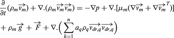
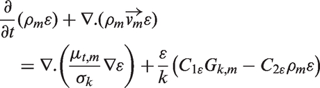
The present study investigated turbulent two-phase flow, so the turbulence model should be properly chosen to capture high gradients exactly. Some researchers have studied different turbulence models and compared the results with experimental data for rotating pumps;^27,28 they concluded that k-ɛ models showed satisfactory agreement. Orszag et al.²⁹ showed that an RNG k-ɛ can predict fluid behavior in flows with swirl more exactly than other k-ɛ turbulent models. The Eulerian multiphase approach in combination with the RNG k-ɛ turbulence model was used in the present study for the numerical simulation. The conservation equations for the qth phases are provided below. The continuity equation for the mixture is

\frac{\partial}{\partial t} (ρ_{m}) + \nabla . (ρ_{m} v_{m}) = 0

(1)

where

v_{m}

is the mass-averaged velocity as

v_{m} = \frac{\sum_{q = 1}^{n} a_{q} ρ_{q} v_{q}}{ρ_{m}}

(2)

and

ρ_{m}

is the mixture density as

ρ_{m} = \sum_{q = 1}^{n} a_{q} ρ_{q}

(3)

and a_q is the volume fraction of phase q.

The momentum equation for the mixture can be obtained by summing the individual momentum equations for all phases as

\frac{\partial}{\partial t} (ρ_{m} v_{m}) + \nabla . (ρ_{m} v_{m} v_{m}) = - \nabla p + \nabla . [μ_{m} (\nabla v_{m} + \nabla {v_{m}}^{T})] + ρ_{m} g + F + \nabla . (\sum_{k = 1}^{n} a_{q} ρ_{q} v_{dr, q} v_{dr, q})

(4)

where n is the number of phases and

F

is a body force.

μ_{m}

is the viscosity of the mixture represented as

μ_{m} = \sum_{k = 1}^{n} a_{q} μ_{q}

(5)

v_{dr, k}

is the drift velocity for secondary phase k as

v_{dr, q} = v_{q} - v_{m}

(6)

The k and ɛ equations describing the mixture turbulence model are

\frac{\partial}{\partial t} (ρ_{m} k) + \nabla . (ρ_{m} v_{m} k) = \nabla . (\frac{μ_{t, m}}{σ_{k}} \nabla k) + G_{k, m} - ρ_{m} ɛ

(7)

\frac{\partial}{\partial t} (ρ_{m} ɛ) + \nabla . (ρ_{m} v_{m} ɛ) = \nabla . (\frac{μ_{t, m}}{σ_{k}} \nabla ɛ) + \frac{ɛ}{k} (C_{1 ɛ} G_{k, m} - C_{2 ɛ} ρ_{m} ɛ)

(8)

The turbulent viscosity, $μ_{t, m}$ , can be computed as

μ_{t, m} = ρ_{m} C_{μ} \frac{k^{2}}{ɛ}

(9)

and the production of turbulence kinetic energy,

G_{k, m}

, is

G_{k, m} = μ_{t, m} (\nabla v_{m} + (\nabla v_{m}) T) : \nabla v_{m}

(10)

Model geometry and boundary conditions

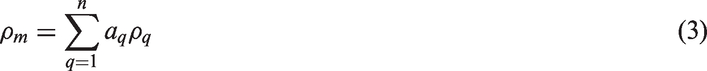
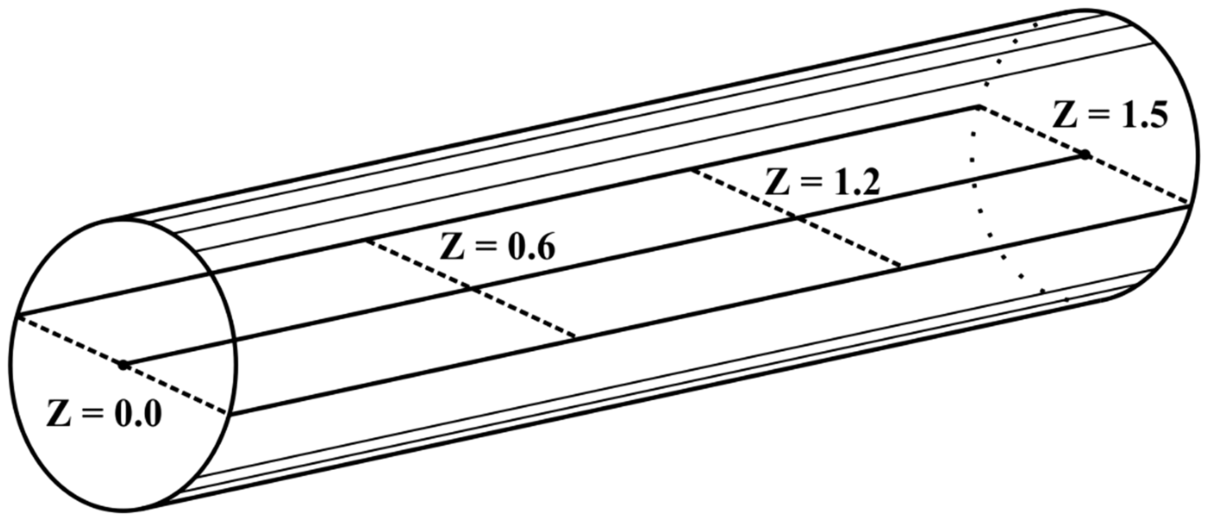
The model geometry consisted of a pipe 1.5 m in length with a constant diameter of 5 cm that has one input and one output. Figure 1 is a schematic of the model geometry.

Figure 1.

Schematic of model geometry.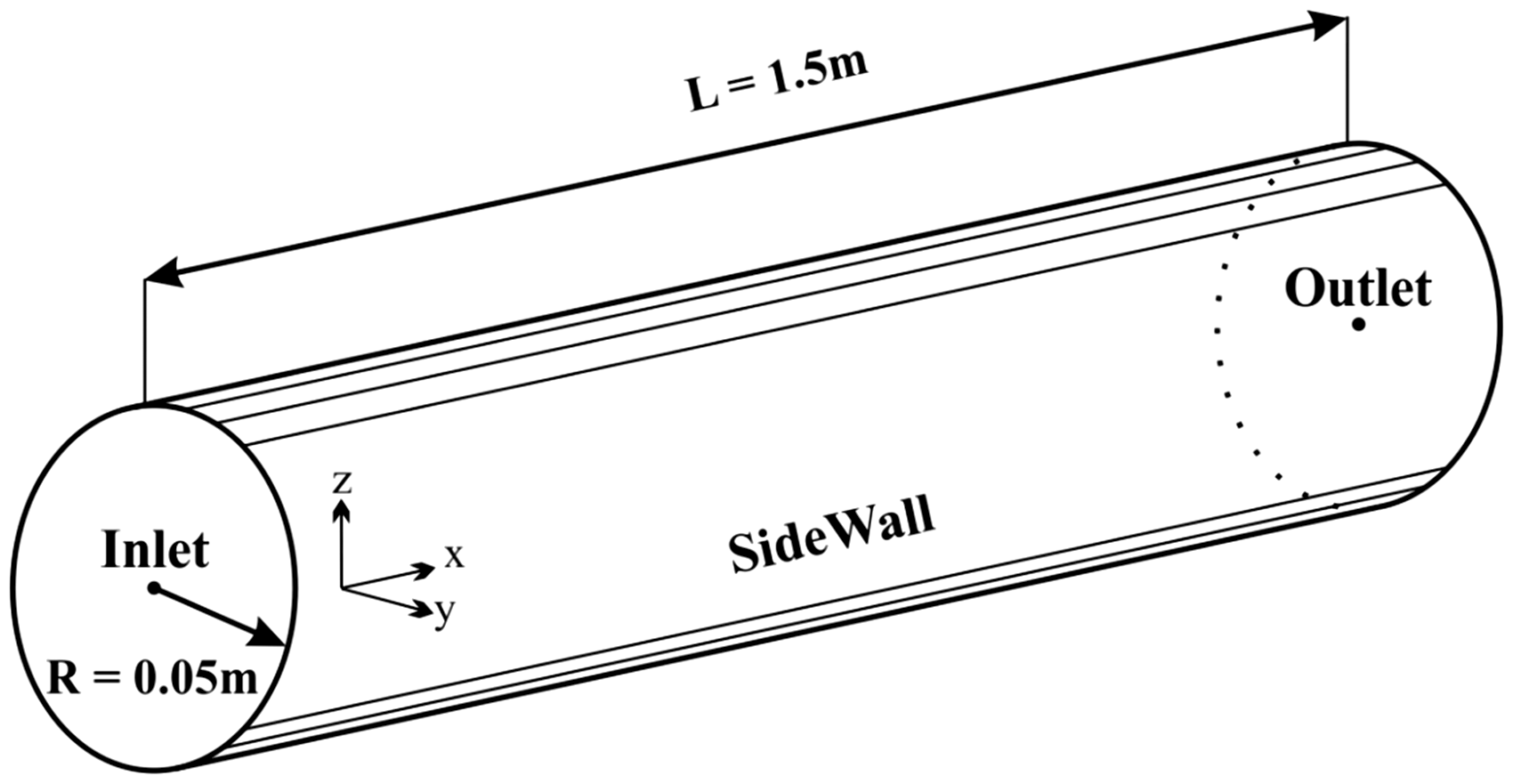

Because this study concentrates on the evolution of a two-phase free vortex in tube-constrained geometry, free vortex flow in the form of a Rankine vortex was assigned at the inlet. Because the velocity and pressure at the outlet boundary are not known in advance, the parameters were calculated by extrapolation from the domain amounts. The flow consisted of water as the solvent phase and oil as the solute phase. Table 1 lists the properties of the boundary conditions and the properties of the Rankine free vortex at the inlet are shown in Figure 2. Note that the diameter of the forced vortex core of the Rankine vortex is 0.6 cm and a free vortex forms at higher diameters.

Table 1.

Properties of model boundary conditions.

Properties	Value
Pipe length (m)	1.5
Pipe diameter (m)	0.05
Axial velocity of inlet flow (m/s)	1.5
Multiplication of tangential velocity in radius of inlet flow (m²/s)	0.005
Water density (kg/m³)	989
Oil density (kg/m³)	830
Oil concentration (ppm)	3000
Oil droplet radius (µm)	400

Figure 2.

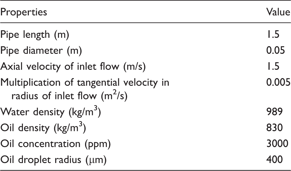
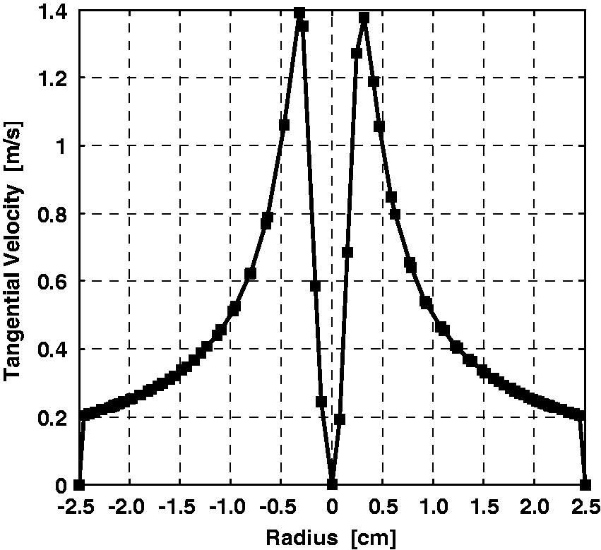
Inlet boundary conditions.

Numerical description

The finite volume method based on the Navier–Stokes equations was employed to discretize the governing equations. Second-order upwind scheme was used for spatial discretization. SIMPLE method was used to solve the discretized equations. The Eulerian multiphase approach combined with a RNG k-ɛ turbulence model was used to model the two-phase flow and turbulence. All the simulations were carried out using OpenFOAM version 4.0.

Validation

Axial turbulent flow in a pipe was simulated to validate the proposed model. A power law relation was used to calculate the velocity profile at the pipe section in the region in which turbulent flow is fully developed³⁰

u - U_{max} = (1 - \frac{r}{D})^{\frac{1}{n}}

(11)

where U_max is the maximum flow velocity in the pipe and occurs at the centerline. Calculation of parameter n is expressed in Schlichting.³⁰ The maximum velocity in the pipe, U_max, is

\frac{U_{max}}{V} = \frac{(2 n + 1) (n + 1)}{2 n^{2}}

(12)

In a turbulent flow in a pipe, the length for the developed flow can be predicted as

L_{h, Turbulent} = 1.359 D ({Re}_{D}) 0.25

(13)

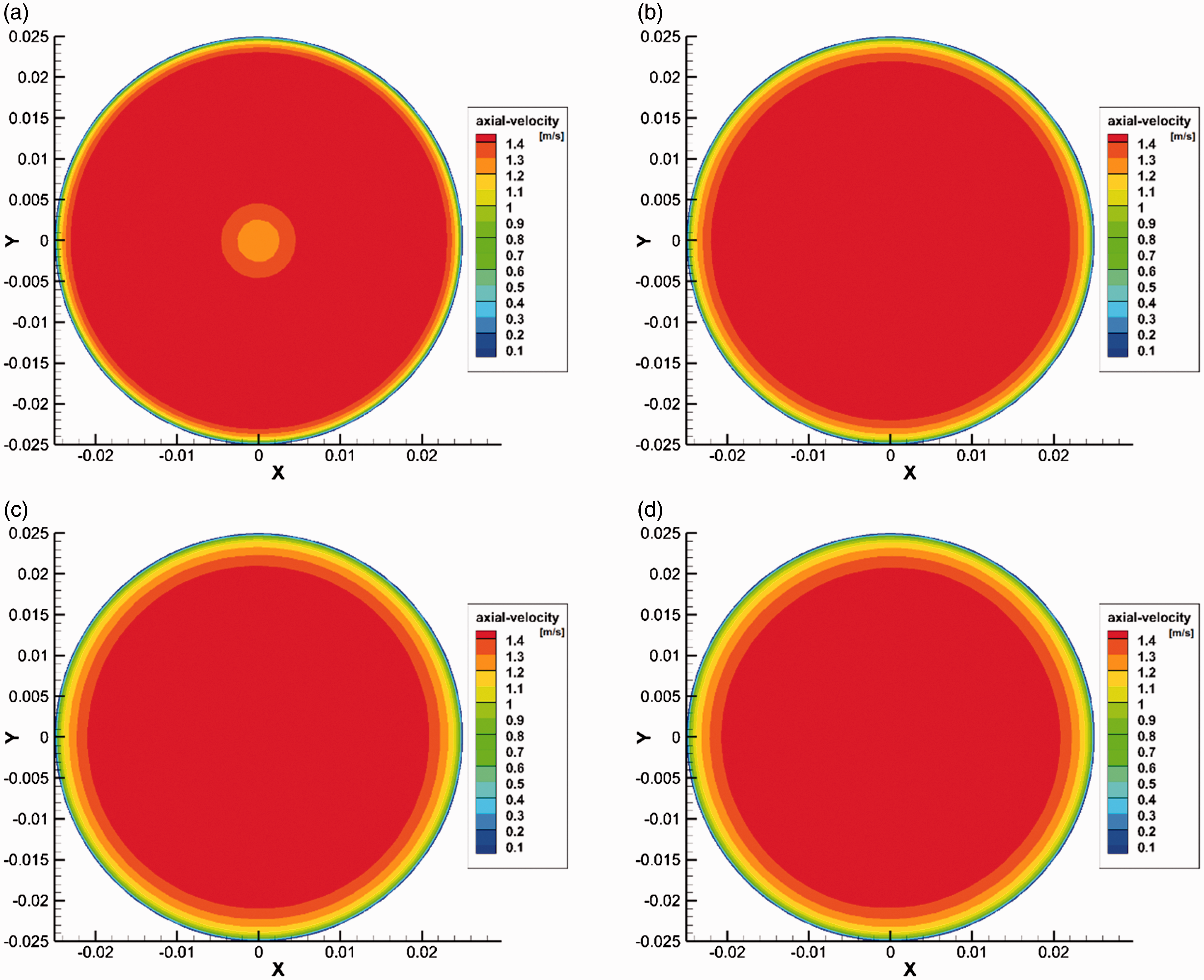
A pipe 1.5 m in length and 5 cm in diameter was chosen and the axial velocity at the inlet was 2 m/s. Comparison of the results of power law relation (11) and the numerical model is shown in Figure 3. Figure 4 shows the velocity distribution in the pipe sections. Figure 5 shows the axes of calculation of velocity at the pipe section.

Figure 3.

Comparison of results of power-law relation and numerical model.

Figure 4.

Velocity distribution in the pipe sections: (a) section z = 0.2 m, (b) section z = 0.6 m, (c) section z = 1.2 m, (d) section z = 1.5 m.

Figure 5.

Axes for calculation of velocity in pipe section.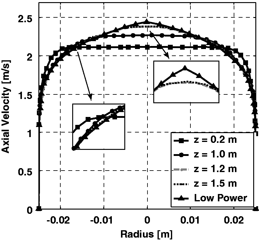

Relation (13) calculates the developed flow length to be about 1.2 m for the pipe and flow condition used for validation. Figure 4 shows the velocity profiles for z = 1.2; at larger values of z they do not change and become constant. There is good agreement between the results of the present model and the power law results, which validates the model.

Grid independence study

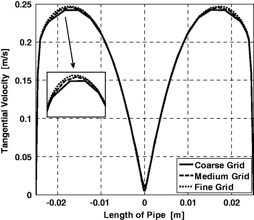
An organized mesh was created over the geometry and three mesh densities were used to study the grid independence. A total of 571,095, 1,175,000, and 1,524,500 cells were used. Figures 6 and 7 show the simulated axial and tangential velocity profiles, respectively, of a single-phase axial vortex flow with an inlet velocity of 1.5 m/s at the outlet of the pipe. In a compromise between high accuracy and low computational cost, the mesh with 1,175,000 cells was selected as having the most acceptable accuracy for the simulations.

Figure 6.

Grid independence at different mesh resolutions for axial velocity.

Figure 7.

Tangential velocity at different mesh resolutions.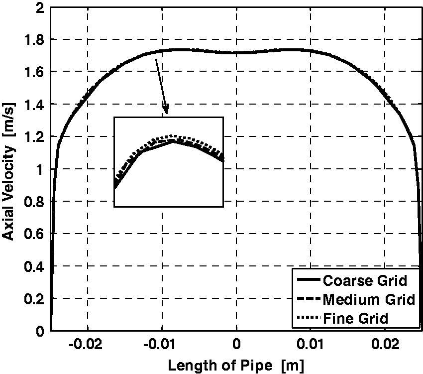

Results and discussion

Tangential velocity distribution

Figure 8 shows the tangential velocity profiles at different sections along the sides of the pipe. At z = 0.2 m section, the free vortex at the inlet evolves into a combination of free and forced vortices with the forced vortex existing at the core. Tangential velocity distribution in a free vortex is proportional to the inverse of the radius; however, in a forced vortex, it is proportional to the radius. Figure 8 indicates that, at z = 0.2 m section, a forced vortex with a radius of 0.01 m from the center of the pipe clearly forms, but in the vicinity of the pipe wall, there exists a free vortex. As the flow continues along the pipe, the radius of the core of the forced vortex increases. The strength of both the forced vortex at the core and the neighboring free vortex weakens from the effect of viscosity. It can be inferred that the development of a free vortex as a stable and independent phenomenon is not possible in a pipe. It can also be concluded that the free and forced vortices in combination produce stable behavior in tube-constrained free vortex flow.

Figure 8.

Tangential velocity profiles for: (a) z = 0 to 1.5 m; and (b) z = 0.2 to 1.5 m.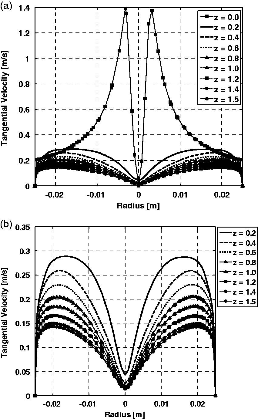

Table 2 shows the maximum tangential velocity at sections for z = 0.2, 0.4, 0.6, 0.8, 1, 1.2, 1.4, and 1.5 m. The radius at which the maximum tangential velocity occurs is also presented. It is clear that the maximum tangential velocity decreases in the streamwise direction from the effect of viscosity. The radius at which maximum velocity occurs increases, demonstrating the evolution of the free vortex structure to a forced vortex structure.

Table 2.

Maximum tangential velocity at different pipe sections.

Pipe section	Maximum tangential velocity (m/s)	Radius of maximum tangential velocity (m)
z = 0.2 m	0.288764	0.0160242
z = 0.4 m	0.259218	0.0181262
z = 0.6 m	0.229383	0.0181262
z = 0.8 m	0.204424	0.0189625
z = 1 m	0.184499	0.0189625
z = 1.2 m	0.165616	0.0197653
z = 1.4 m	0.150113	0.0198646
z = 1.5 m	0.143566	0.0198646

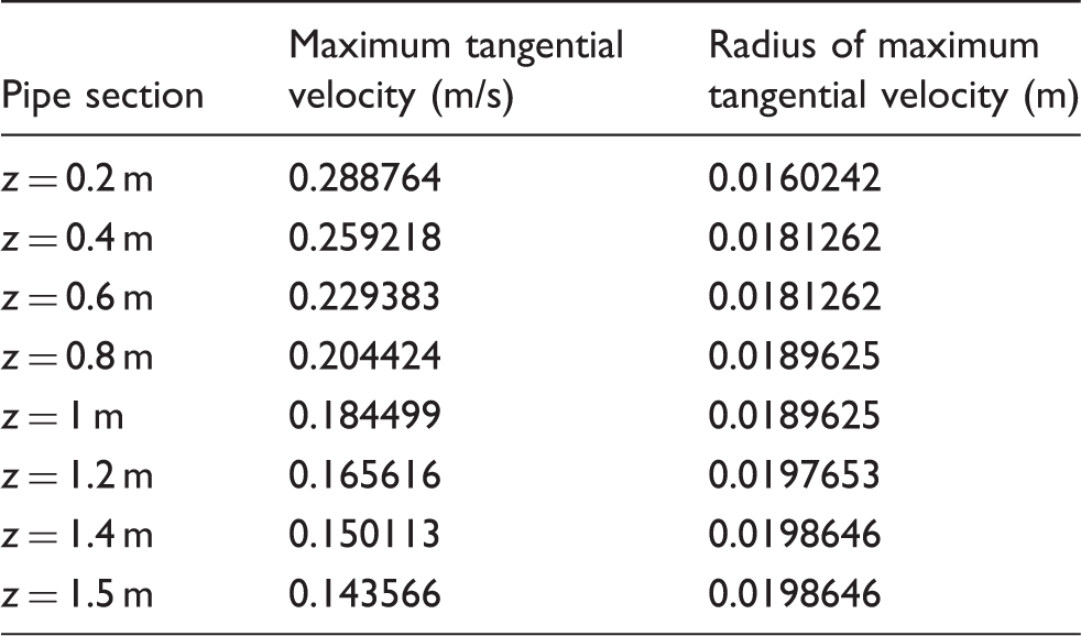
The results show a decrease of 10.23%, 20.56%, 29.21%, 36.11%, 42.65%, 48.02%, and 50.28% at maximum tangential velocities at z = 0.4, 0.6, 0.8, 1, 1.2, 1.4, and 1.5 m, respectively, compared with the maximum tangential velocity at z = 0.2 m. The maximum tangential velocity decreased from z = 0.2 m to z = 1.5 m by 50.28% and the radius at which it occurred increased.

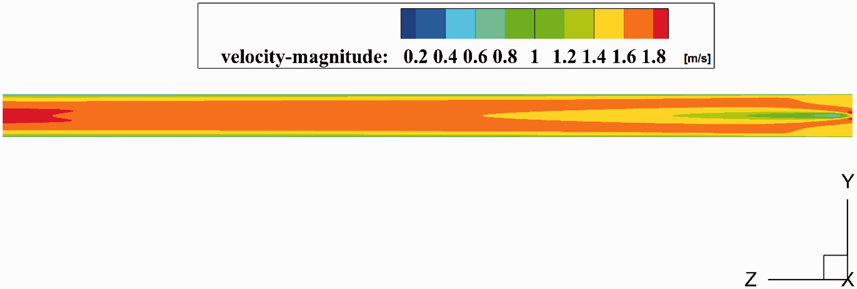
The contour of the tangential velocity in the longitudinal sections and the magnitude of mixture velocity are shown in Figures 9 and 10, respectively. It was observed that, as the flow passes down the length of the pipe, the structure of the free vortex at the point at which the velocity around the core is greater than the velocity at larger diameters forms combined forced and free vortices. This is clearly shown at the outlet section; the tangential velocity increases as the diameter increases (forced vortex structure) up to a specific diameter, above which the velocity decreases as the diameter increases (free vortex structure).

Figure 9.

Contour of tangential velocity at longitudinal section.

Figure 10.

Contour of mixture velocity magnitude.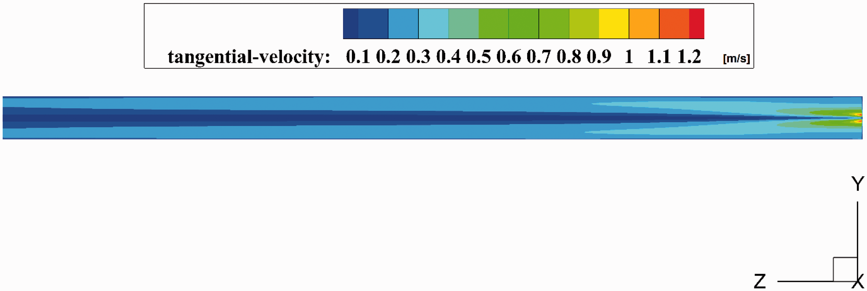

Discrete phase concentration

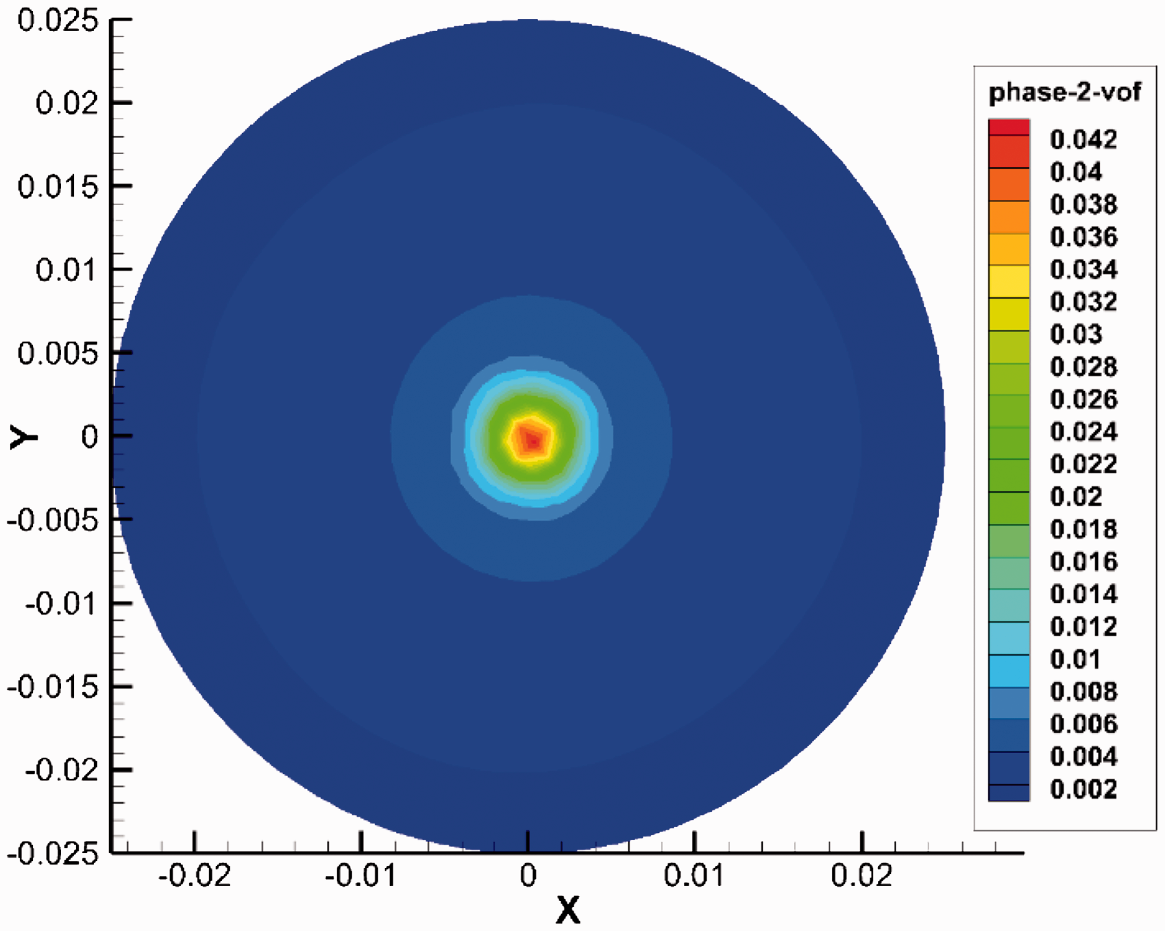
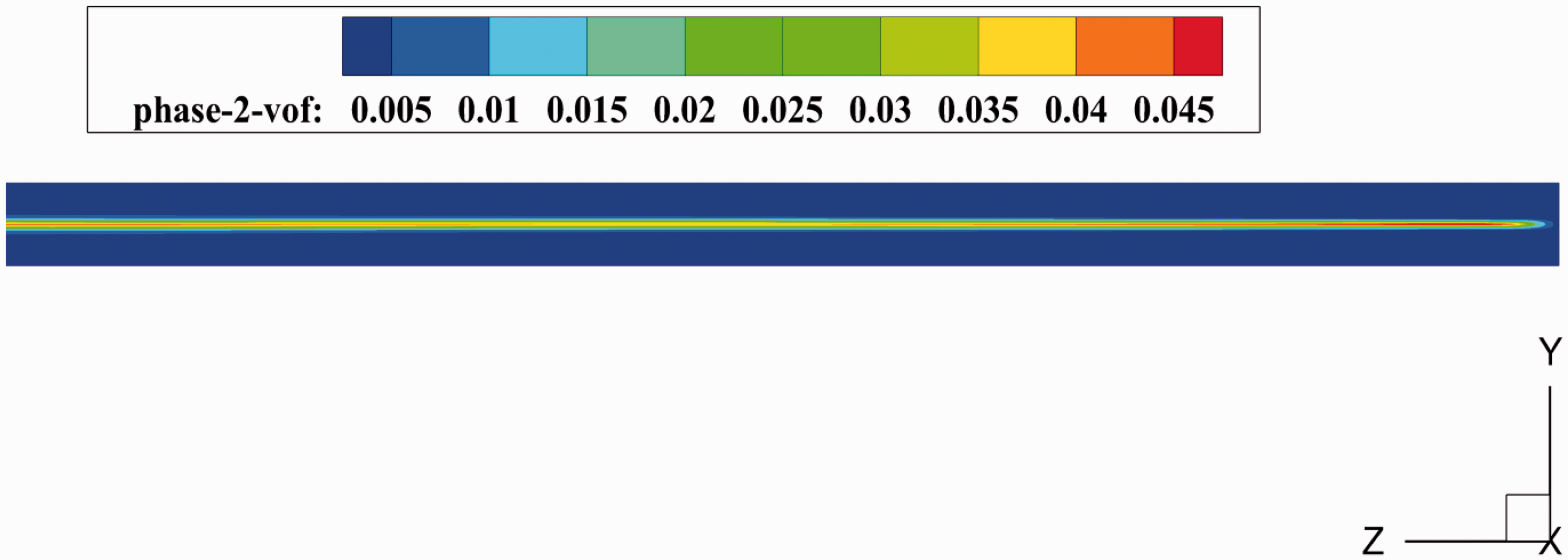
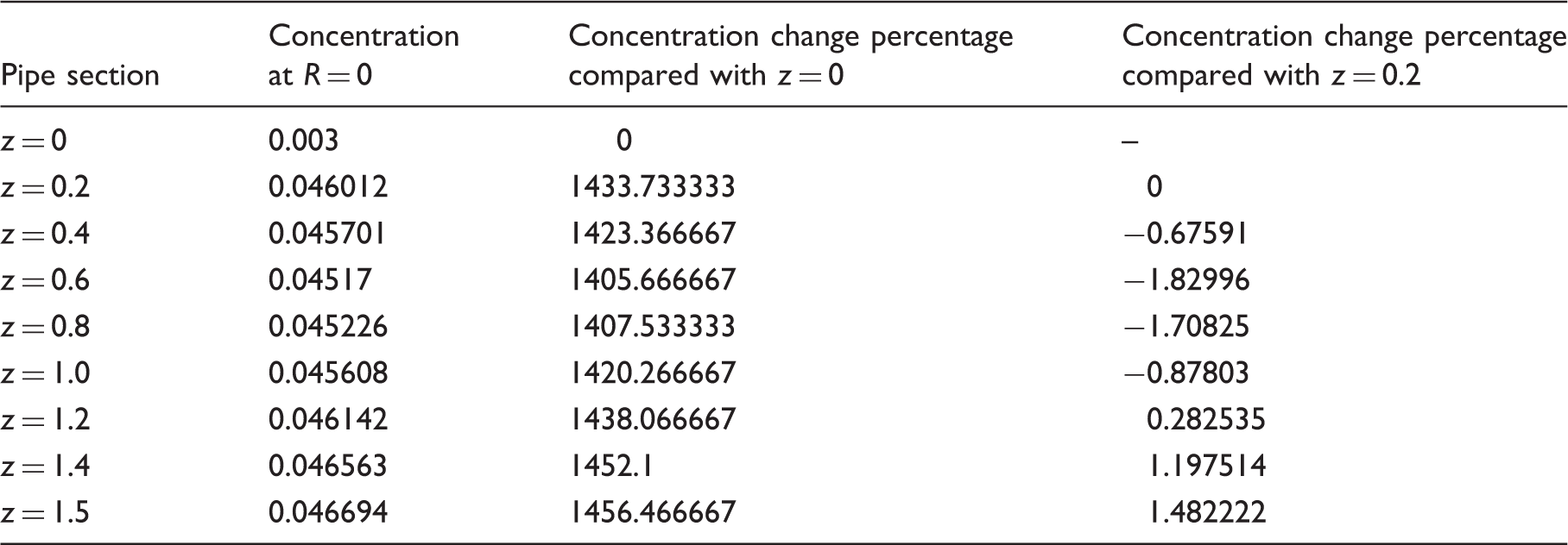
Figure 11 shows the concentration of the discrete phase at different sections along the pipe. Figure 12 shows the concentration contour at the outlet section of the pipe. Figure 13 shows the contour in the longitudinal section for the discrete phase concentration. The concentration of the second (discrete) phase is highest at the center of the pipe at the vortex core. Table 3 shows the discrete phase concentration at the center of the pipe in different sections. The maximum concentration of discrete oil in the center of the diagram is a sign of the power of the vortex. At the beginning, the vortex has higher tangential velocity, so maximum separation occurs at the center.

Figure 11.

Volume fraction of discrete phase in different sections.

Figure 12.

Second phase volume fraction contour for z = 1.5 m.

Figure 13.

Contour of second phase concentration.

Table 3.

Discrete phase concentration at pipe center in different sections.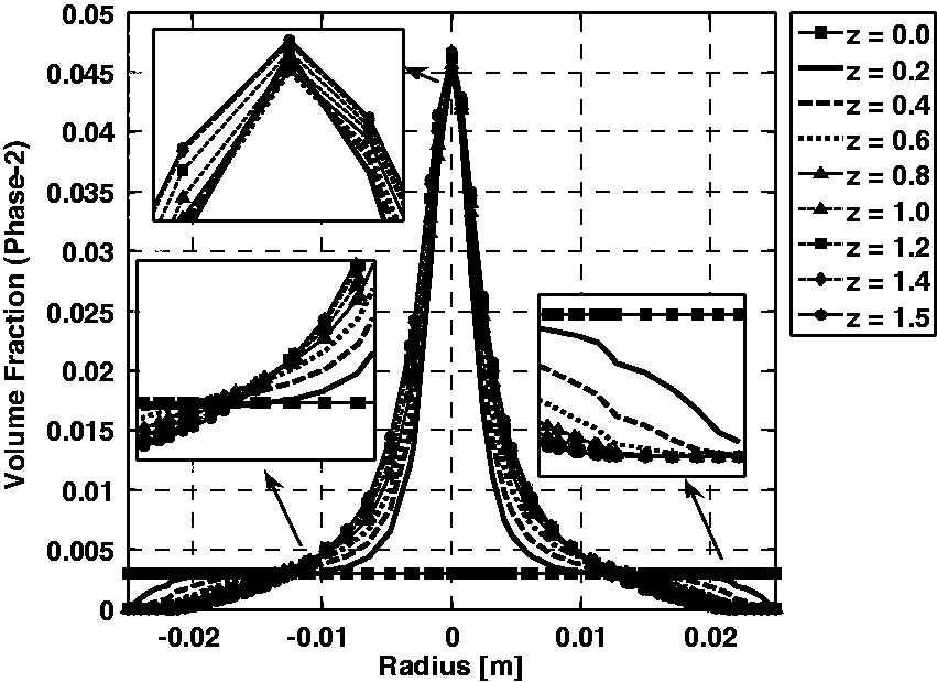

Pipe section	Concentration at R = 0	Concentration change percentage compared with z = 0	Concentration change percentage compared with z = 0.2
z = 0	0.003	0	–
z = 0.2	0.046012	1433.733333	0
z = 0.4	0.045701	1423.366667	−0.67591
z = 0.6	0.04517	1405.666667	−1.82996
z = 0.8	0.045226	1407.533333	−1.70825
z = 1.0	0.045608	1420.266667	−0.87803
z = 1.2	0.046142	1438.066667	0.282535
z = 1.4	0.046563	1452.1	1.197514
z = 1.5	0.046694	1456.466667	1.482222

To separate the discrete phases, the flow was exposed to an axial vortex. Continuation of the vortex stabilizes the axial vortex and it moves from a transitional to a stable state (at which the rate of variation is not intense). This occurs as the stream continues, where it can be observed that the concentration of the discrete oil phase near the pipe wall decreases and it moves toward the vortex core. This behavior increases the concentration near the core.

As the axial vortex continues, the power and strength of the vortex decrease compared with the transitional state. Continuation of the vortex as time passes influences the stream and causes the discrete phase to accumulate, resulting in further separation and an increase in concentration at the vortex core. The continuation and separation of the discrete phase in the streamwise direction increases the maximum concentration of the discrete phase at the vortex core at the pipe outlet. If a smaller pipe with a diameter that approximately equals the vortex core diameter is used, the second phase can be segregated from the base phase. This could be an effective method of segregation in multi-phase flows because the combined free and forced vortices become stable in tube-constrained free vortex flow.

In a free vortex flow, particles are scattered in a way that particles with lower density (as compared to dominant phase of the flow) are collected in vortex core and heavier particles are observed near pipe walls. For the reason that oil phase has smaller density than dominant phase, and due to the force which is implemented on the oil phase droplets (centrifugal effect of the vortex flow on the fluid particles), they are gathered in vortex core. That is why the concentration of the second (discrete) phase is highest at the center of the pipe at the vortex core. At the beginning, the vortex has higher tangential velocity, so maximum separation occurs at the center. To separate the discrete phases, the flow was exposed to an axial vortex. Continuation of the vortex stabilizes the axial vortex. This occurs as the stream continues, where it can be observed that the concentration of the discrete oil phase near the pipe wall decreases and it moves toward the vortex core. This behavior increases the concentration near the core. As the axial vortex continues, the power and strength of the vortex decreases compared with the transitional state. Continuation of the vortex influences the stream and causes the discrete phase to accumulate, resulting in further separation and an increase in the concentration at the vortex core.

Conclusion

Numerical simulation was used to model the evolution of a free vortex structure in a two-phase flow in tube-constrained geometry. The model was validated using an empirical relation for turbulent flows. Assigning a Rankine vortex to the inlet boundary allowed investigation of the evolution of an oil–water two-phase flow in a free vortex structure.

It was shown that at 0.2 m from the inlet, a forced vortex core clearly forms and extends. As it extends to larger radiuses, the strength of both the free and forced vortices, the tangential velocity, decreases in response to the effects of viscosity. The core of the forced vortex also extends and the velocity at higher radiuses decreases as the fluid flows down the side of the pipe.

The results also show that the concentration of the discrete phase is at a maximum at the center of the pipe at the core of the vortex. This concentration increases as the flow continues down the length of the pipe after the vortex reaches a stable state. The concentration at the core is at a maximum at the outlet.

It can be inferred that the production of a free vortex as a stable and independent phenomenon is not possible. It can also be concluded that the combined free and forced vortices can produce stable behavior in the tube-constrained free-vortex flow. It was shown that this combination is a useful and effective method for separation of two-phase flows that are typical of the petroleum industry.

Footnotes

Declaration of conflicting interests

The author(s) declared no potential conflicts of interest with respect to the research, authorship, and/or publication of this article.

Funding

The author(s) received no financial support for the research, authorship, and/or publication of this article.

References

Tennekes

Lumley

. A first course in turbulence, Cambridge, MA: MIT Press, 1972.

Hunt

JCR

. Vorticity and vortex dynamics in complex turbulent flows. Trans Can Soc Mech Engrs 1987; 11: 21.

Hussain

Melander

. Understanding turbulence via vortex dynamics. In: The Lumley symposium: Studies in turbulence, New York: Springer, 1991, pp. 157–178.

Lamb

. Hydrodynamics, Mineola, NY: Dover, 1945.

Lugt

. The dilemma of defining a vortex. In: Recent development in theoretical and experimental fluid mechanics, New York: Springer, 1979, pp. 309–321.

Chong

Perry

Cantwell

. A general classification of three-dimensional flow field. Phys Fluid A 1990; 2: 765.

Hunt JCR, Wary AA and Moin P. Eddies, streams, and convergence zones in turbulent flows. Center for Turbulence Research Report CTR-S88, 1988, p. 193.

Jeong

Hussain

. On the identification of a vortex. J Fluid Mech 1995; 285: 69–94.

Doligalski

Smith

Walker

JDA

. Vortex interactions with walls. Annu Rev Fluid Mech 1994; 26: 573–616.

10.

Zheng

. A consistent boundary condition for vorticity – Stream function simulation of wall-bounded vortex flow. Appl Math Comput 2008; 206: 205–213.

11.

Chen

et al.

Experimental and numerical investigation of free surface vortex. J Hydrodyn 2008; 20: 485–491.

12.

Chen

et al.

Formation and influencing factors of free surface vortex in a barrel with a central orifice at bottom. J Hydrodyn 2009; 21: 238–244.

13.

Chen

et al.

Hydraulic characteristics of vertical vortex at hydraulic intakes. J Hydrodyn B 2007; 19: 143–149.

14.

Hite

Mih

. Velocity of vertical vortices at hydraulic intakes. J Hydraulic Eng ASCE 1994; 120: 284–297.

15.

Kabiri-Samani

Borghei

. Effects of anti-vortex plates on air entrainment by free vortex. Scient Iran A 2013; 20: 251–258.

16.

Jain

Ranga Raju

Garde

. Vortex formation at vertical pipe intakes. J Hydraul Div ASCE 1978; 104: 1429–1448.

17.

Denny

. An experimental study of air-entraining vertices in pump. J Instn Mech Engrs 1956; 170: 106–116.

18.

Daggett

Keulegan

. Similitude conditions in free-surface vortex formation. J Hydraul Div ASCE 1974; 170: 1565–1581.

19.

Y-j

Guo

Z-z

. Flow upstream of intake. J Hydrodyn A 1989; 4: 74–78.

20.

Henderson

Gwynllywa

Barenghi

. Particle tracking in Taylor–Couette flow. Eur J Mech B 2007; 26: 738–748.

21.

El-Naggar

Kholeif

. Motion of a small spherical particle in a fluid vortex. J Basic Appl Sci Res 2012; 2: 3631–3635.

22.

Domon

Watanabe

. Mass transport by a vortex ring. J Phys Soc Jpn 2000; 69: 120–123.

23.

Uchiyama T and Yagami H. Vortex simulation for the interaction between a vortex ring and solid particles. In: Proceedings of 6th international conference on multiphase flow, Leipzig, 2007.

24.

Uchiyama

Yagami

. Numerical simulation for the collision between a vortex ring and solid particles. Powder Technol 2008; 188: 73–80.

25.

Candelier

Angilella

Souhar

. On the effect of the Boussinesq-Basset force on the radial migration of a Stokes particle in a vortex. Phys Fluids 2004; 16: 1765–1777.

26.

Salari

Karmozdi

Maddahian

et al.

Analytical study of single particle tracking in both free and forced vortices. Scient Iran B 2013; 20: 351–358.

27.

Hartmann

Derksen

Montavon

et al.

Assessment of large eddy and RANS stirred tank simulations by means of LDA. Chem Eng Sci 2004; 59: 2419–2432.

28.

Zakrzewska

Jaworski

. CFD modelling of turbulent jacket heat transfer in a Rushton turbine stirred vessel. Chem Eng Technol 2004; 27: 237–242.

29.

Orszag SA, Yakhot V, Flannery WS, et al. Renormalization group modeling and turbulence simulations. In: International conference on near-wall turbulent flows, Tempe, AZ, USA, 1993.

30.

Schlichting

. Boundary layer theory, 4th ed. New York: McGraw-Hill Book Co., Inc., 1960.

Two-phase flow separation in axial free vortex flow

Abstract

Keywords

Introduction

Model

Governing equations

Model geometry and boundary conditions

Numerical description

Validation

Grid independence study

Results and discussion

Tangential velocity distribution

Discrete phase concentration

Conclusion

Footnotes

Declaration of conflicting interests

Funding

References