Sage Journals: Discover world-class research

Abstract

A gust wind tunnel designed to generate predictable wind patterns for aerodynamic testing was developed. From the detailed wind speed measurements in the test section, a wind gust model was constructed to characterize the time and positional variation of the wind speed and direction. The wind gust model, verified using hot-wire velocimetry, exhibited an error of less than 1%. The constructed wind gust model enabled the identification of the flight dynamics of objects in free flight, such as flapping insects. The dynamic model of a bumblebee flying in gusty winds was analyzed in a wind tunnel, and the transfer functions for the pitch angle and z-directional velocity in response to gust inputs were identified. Singular value analysis of the identified dynamics revealed that the control gain was adjusted either to decrease gust responses or improve robust stability according to wind conditions.

Keywords

gust generator wind tunnel control system identification wind gust model insect flight flight control

Introduction

Unmanned aerial vehicles (UAVs) have recently been used in a wide range of fields. One such application involves carrying payloads, thereby replacing manned aircraft in certain applications. In particular, micro unmanned aerial vehicles (MAVs) can access confined spaces in which manned aircraft cannot operate. Although there is a strong demand for MAVs to replace manned aircraft in certain operations, designing an MAV that can fly stably under turbulent wind conditions while maintaining control of its posture, all within the constraints of limited payload capacity and size, presents a significant challenge.

In the MAV design process, information based on the biomimetics of small insects enhances the flight performance of MAVs. Insects have performed flight tasks under turbulent wind conditions that humans have yet to accomplish. Therefore, studies on insect flights have been conducted to apply control systems to manmade MAVs.

The aerodynamic characteristics of flapping wings at low Reynolds numbers were modeled in wind tunnel experiments.¹ For flapping insects, the leading-edge vortex generated a large lift force. This effect was confirmed by experiments in which the MAVs were flapped.¹ Structural analyses of insect wings were performed to mimic insect flight mechanisms.^2,3 Both flapping insects and flapping MAVs are inherently unstable.^4,5 By varying the flap amplitude and offset of the flapping linkage,⁶ as well as the stroke plane and wing twist,⁷ the control moment required for stabilization was generated. In Ref.,⁸ an attempt was made to stimulate flight muscles by electrical stimulation to reproduce the flapping motion of insects. Additionally, studies have been conducted on the development of flapping robots that are relatively larger than insects, and wind tunnel tests.^9–17 Recent research includes the aerodynamic optimization of flapping wings,¹⁸ analysis of clapping wing mechanisms,¹⁹ and the development of MAVs with cyclorotors inspired by insect flight dynamics.^20,21 Therefore, research on the aerodynamics and structure of insect flights has increased. 　

The dynamics of flying insects under disturbed flow conditions were also investigated. Although high-performance and stable flight has been observed,^22–25 it is difficult to study the flight control system directly, which is implemented in the muscle nervous system. The responses of the tethered insects to visual information or wind velocity changes were observed.^4,26–28 However, ensuring that tethered insects behave exactly as they do under free-flight conditions in natural environments is difficult.

Despite progress in insect flight control research, neuromuscular system flight strategies under gusty disturbances remain unclear. To analyze the flight dynamics of insects, it is necessary to model their flight in conditions that mimic their natural environment, allowing them to fly freely in turbulent winds. The dynamic model of insects flying under turbulent wind conditions can be identified by analyzing the input and output of the system. The inputs are the wind speed and direction encountered by the insect, and the outputs are the position and attitude of the insect. The time histories of both inputs and outputs must be accurately measured to obtain an insect flight model. However, directly measuring the variable wind conditions encountered by a free-flying object requires installing sensors, recording devices, or wireless modules on the flying object, which is virtually impossible for insect-sized objects. Therefore, a new system is required to measure the wind encountered by free-flying objects without affecting the flow field or altering their dynamics.

Previous turbulent wind tunnels generated isolated gusts with a definite time history^29,30 or continuous gusts with a guaranteed statistical value.^31–33 However, it is difficult to identify the wind conditions encountered by insects flying freely in existing turbulent wind tunnels, which is necessary for flight dynamics identification.

This study aims to develop a method for analyzing insect dynamics and control using wind tunnels. First, a free-flight wind tunnel was developed to generate repeatable wind disturbances with a definable time-variation history (Section 2). This allowed measurement of the wind speed and direction encountered by a flying object within the test section. For the output acquisition, the motion and posture of a flying object can be obtained using a stereo camera system with a high-speed camera. In addition, free-flight experiments on bumblebees were conducted in a turbulent wind tunnel to model the flight dynamics of bees flying under gusty wind conditions (Section 3). Finally, the control system design strategies of the bumblebees were analyzed.

Development of the wind tunnel with gust generator

A wind tunnel that generates periodic gusts as input signal for the dynamic identification of flying objects was developed. The spatial distribution and time variation of the wind speed were modeled by measuring the wind velocity in the test section, and the accuracy of the constructed model was evaluated.

Gust generator

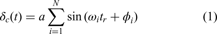
A gust generator was installed in the suction-type wind tunnel (Figure 1). The test section was 0.2 m wide, 0.2 m high, and 0.54 m long. The gust vane was made from a 2 mm-thick aluminum flat plate that is 0.18 m wide and 0.15 m long. A two-dimensional gust was generated by an oscillating vane around the 0.83 chord length position. The vane was moved by a servomotor (Kondo Kagaku, KRS-5032HV ICS) with commands generated by the Arduino Uno. To precisely identify flying object dynamics in response to gust input, the bandwidth of the gust must be high to excite the dynamic modes and make the responses visible. In this study, the command of the vane angle $δ_{c} [\circ]$ is defined as follows:

δ_{c} (t) = a \sum_{i = 1}^{N} \sin (ω_{i} t_{r} + ϕ_{i})

(1)

t_{r} = \mod (t, T_{c})

(2)

where a is the amplitude,

ω_{i}

is the angular velocity,

ϕ_{i}

is the initial phase of the i^th oscillating element, N is the total number of oscillating elements, and

\mod (t, T_{c})

is the remainder of t divided by

T_{c}

. The single-command history of the period

T_{c}

was repeated several times.

Figure 1.

Wind tunnel with gust generator.

Let $v_{g} (x, y, z, t)$ be the wind velocity vectors at positions $(x, y, z)$ and time t. If the following equation is satisfied at any position in the test section, the wind speed and direction that the flying object encounters can be determined from the measured object position and wind distribution model for a period $T_{c}$ that should be formulated.

v_{g} (x, y, z, t) = v_{g} (x, y, z, t + j T_{c}), j = 0, 1, 2, \dots

(3)

Wind speed distribution

The target dynamics of this study were based on those of insect flies. The bandwidth of the gust input should be determined based on the frequency of the bee flight to be analyzed. The bee response to gust input may contain high-frequency dynamics at the flapping frequency, which is above 100 Hz. However, it is difficult to vibrate and measure the attitude of the bee at this frequency. Therefore, the vibration frequency and amplitude of the vane were determined through preliminary flight tests to ensure that the generated wind field could effectively excite and capture the relevant bee dynamics. Table 1 lists the determined vane oscillation parameters. The oscillation of the vane had four frequencies: 0.1, 0.7, 1.3, and 1.8 Hz. The time histories of these commands are presented in Figure 2. The time histories corresponding to these control commands over a 5 s interval were repeated cyclically, as illustrated in Figure 2.

Figure 2.

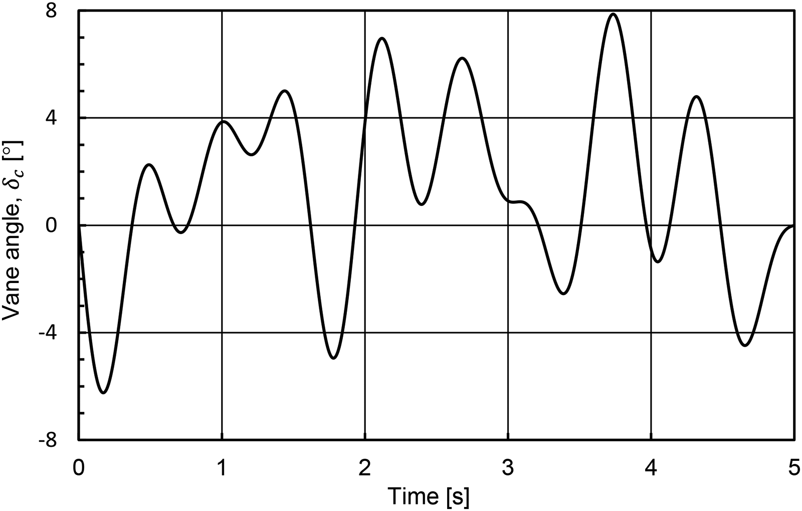
Single time history of the vane angle command.

Table 1.

Parameter values of the vane command history.

Parameter	Value
N	4
$a$ [°]	2.5
$ω_{1}$ , $ω_{2}$ , $ω_{3}$ , $ω_{4}$ [rad/s]	0.628, 4.40, 8.17, 11.3
$ϕ_{1}$ , $ϕ_{2}$ , $ϕ_{3}$ , $ϕ_{4}$ [rad]	$π$ , 0, 0, 0

The gust distribution and time history were measured to construct the wind gust models. The X-type probe of a hot-wire anemometer (KANOMAX, Smart CTA Model 7250) was inserted at the measurement point on the grid to simultaneously measure the wind velocity in the X- and Z-directions. (Figure 3). The time histories of wind velocity were measured at 910 grid points: five in the X-axis direction, 14 in the Y-axis direction, and 13 in the Z-axis direction. The mainstream velocity was set to 1.5 m/s. This was lower than the flying speed of the bees, and the bees could fly upwind in the test section. This speed was optimized through trial and error to ensure that sufficient flight data could be captured.

Figure 3.

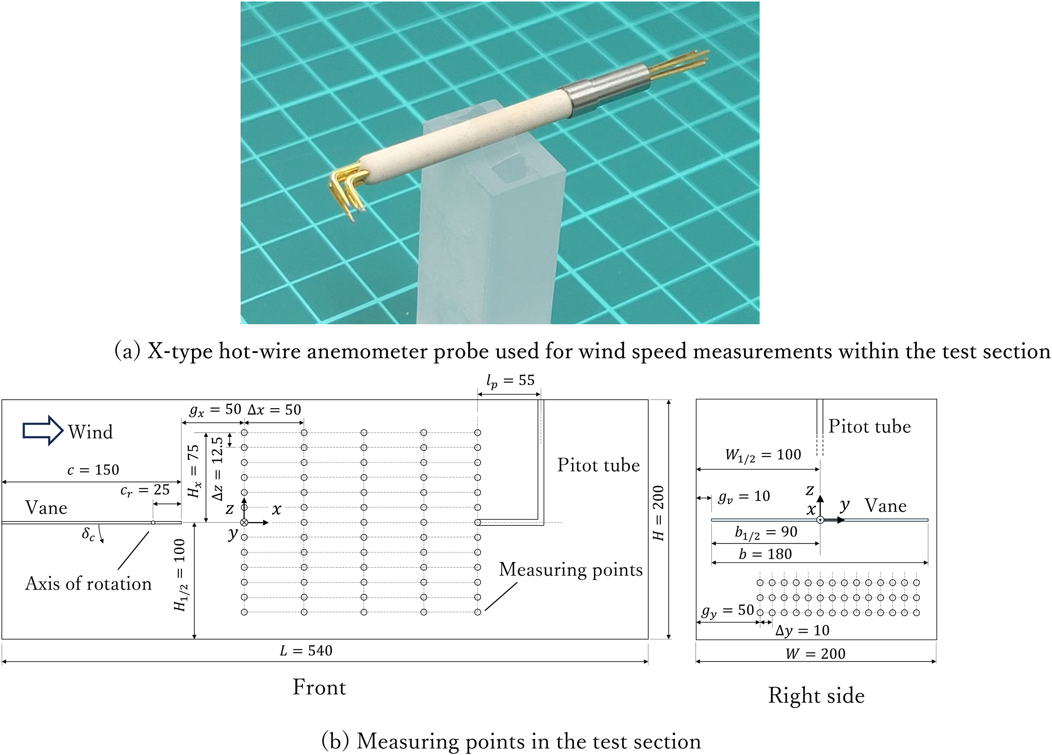
Equipment and layout for wind speed measurements. (a) X-type hot-wire anemometer probe used for wind speed measurements within the test section. (b) Measuring points in the test section.

The ensemble averages of measured wind speed are calculated as follows:

{\bar{v}}_{g} (x, y, z, t) = \frac{1}{N_{s} + 1} \sum_{j = 0}^{N_{s}} v_{g} (x, y, z, t + j T_{c}) (0 \leq t < T)

(4)

Figure 4 shows the ensemble averages of the measured wind speeds at $y = 0$ mm. The wind profile generated upwind of the test section shifted downwind while maintaining its shape. However, the flow at the same height as the vane, $z = 0$ mm, was disturbed.

Figure 4.

Measured wind speed history at y = 0 mm during vane oscillation. (a) z = -50 mm. (b) z = 0 mm. (c) z = 50 mm.

The similarity of the wind profiles was evaluated by cross-correlation along the flow direction on the longitudinal plane of the wind tunnel center ( $y = 0 mm$ ). Cross-correlations were calculated as follows:

C (τ)_{x y} = \frac{1}{T} \int_{0}^{T} (\frac{x (t)}{{‖ x (t) ‖}_{p}}) (\frac{y (t + τ)}{{‖ y (t) ‖}_{p}}) d t

(5)

‖ ∙ (t) ‖_{p} = \sqrt{lim_{T \to \infty} \frac{1}{T} \int_{0}^{T} ∙ {(t)}^{2} d t}

(6)

The cross-correlation of the wind speed at x = 0 (the most upwind measuring position) to x = 50, 100, 150, and 200 mm (the downwind measuring positions of the same z-axis value) was analyzed. The maximum cross-correlation values and lag times at the maximum cross-correlation are shown in Figure 5. The lag time increased gradually as the flow moved downwind. This indicates that the wind profiles shifted downwind while maintaining the wind profile. 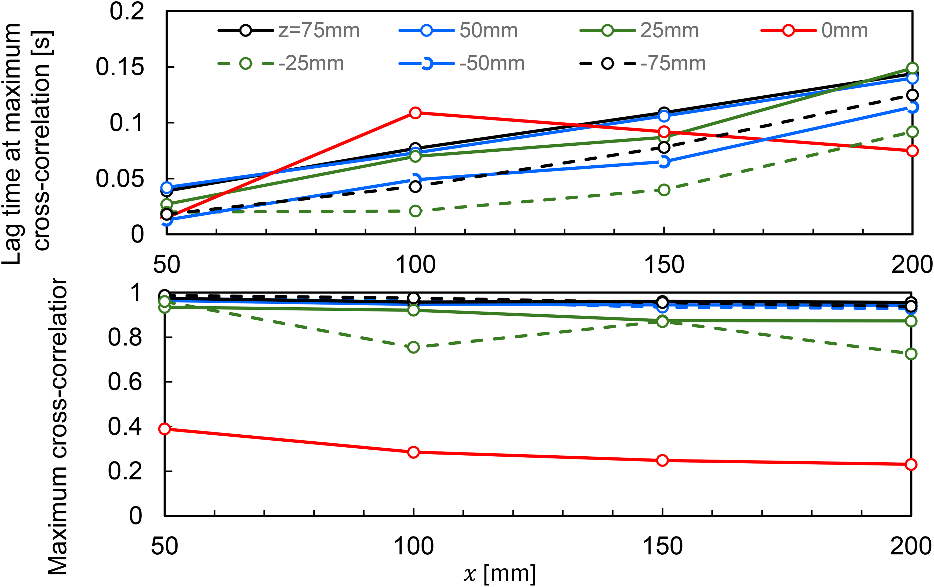However, the flow at the same height as the vane, $z = 0 mm$ , did not exhibit this tendency. The maximum cross-correlation values were smaller than those at other z positions. A disturbed flow was generated from the trailing edge of the vane, which increased the flow uncertainties.

Figure 5.

Cross-correlation of wind speed to the most upwind profile (x = 0 mm).

Wind gust model

The analysis of the measured wind histories demonstrated the reproducibility of the wind profile. Wind speed has a strong correlation with the surrounding position. The wind speed model was constructed by interpolating the wind speed at the vertices of the rectangle containing the modeling point (Figure 6, Eqs. (7)).

\begin{aligned} v_{g_{m o d e l}} (x, y, z, t) = & [{\bar{v}}_{g_{1}} (t_{r}) \times (L_{x} - x_{r}) (L_{y} - y_{r}) z_{r} + {\bar{v}}_{g_{2}} (t_{r}) \times (L_{x} - x_{r}) (L_{y} - y_{r}) (L_{z} - z_{r}) \\ + {\bar{v}}_{g_{3}} (t_{r}) \times x_{r} (L_{y} - y_{r}) (L_{z} - z_{r}) + {\bar{v}}_{g_{4}} (t_{r}) \times x_{r} (L_{y} - y_{r}) z_{r} \\ + {\bar{v}}_{g_{5}} (t_{r}) \times (L_{x} - x_{r}) y_{r} z_{r} + {\bar{v}}_{g_{6}} (t_{r}) \times (L_{x} - x_{r}) y_{r} (L_{z} - z_{r}) \\ + {\bar{v}}_{g_{7}} (t_{r}) \times x_{r} y_{r} (L_{z} - z_{r}) + {\bar{v}}_{g_{8}} (t_{r}) \times x_{r} y_{r} z_{r}] / (L_{x} L_{y} L_{z}) \end{aligned}

(7)

Figure 6.

Grid point configuration used for wind speed modeling.

$t_{r}$ denotes the time from the start of the repeated vane angle history (Eq. (2)). $x_{r}, y_{r}, and z_{r}$ represent the distances from the origin of the rectangle. $L_{x}, L_{y}, and L_{z}$ denote the lengths of the sides of the rectangles. ${\bar{v}}_{g_{i}}$ denotes the ensemble averages and Eq. (4) of the measured wind speed at the vertex point $p_{i}$ . Eq. (7) is a velocity model weighted by the cuboid volume corresponding to each grid point. The position of the flying object in the wind-tunnel test section was measured using a camera. Therefore, the gust input encountered by a flying object can be obtained by constructing the disturbance model shown in Eq. (7) and the position of the bee was measured without a direct measurement.

The smallest rectangle was suitable for precise modeling. When the smallest rectangle could be constructed from the measured points, $L_{x}, L_{y}, and L_{z}$ became 50, 10, and 12.5 mm, respectively. The modeling errors were evaluated by comparing the model and measured wind speeds. In the evaluation, the wind speed, which was not used for modeling, should be compared. A rectangle twice the size of the smallest rectangle was used for interpolation. $L_{x}, L_{y}, and L_{z}$ were 100, 20, and 25 mm, respectively, and the evaluation points were at the center of the rectangle.

The modeling error is evaluated as follows:

\begin{aligned} J_{v} (x, y, z) = \frac{{‖ v_{g_{m o d e l}} (x, y, z, t) - v_{g_{s a m p l e}} (x, y, z, t) ‖}_{p}}{{‖ v_{g_{s a m p l e}} (x, y, z, t) - v_{g_{a v}} (x, y, z) ‖}_{p}} \times 100 \end{aligned}

(8)

where

v_{g_{s a m p l e}}

represents a single measured wind speed history without an ensemble average and

v_{g_{a v}}

represents the time average of

v_{g_{s a m p l e}}

. Figure 7 shows the modeling error distributions calculated using Eq. (8) on the horizontal plane. Figure 8 shows the average modeling error in the x-y plane. The modeling error behind the vane, z = 0 mm, was large owing to the disturbance generated by the trailing edge of the vane.

Figure 7.

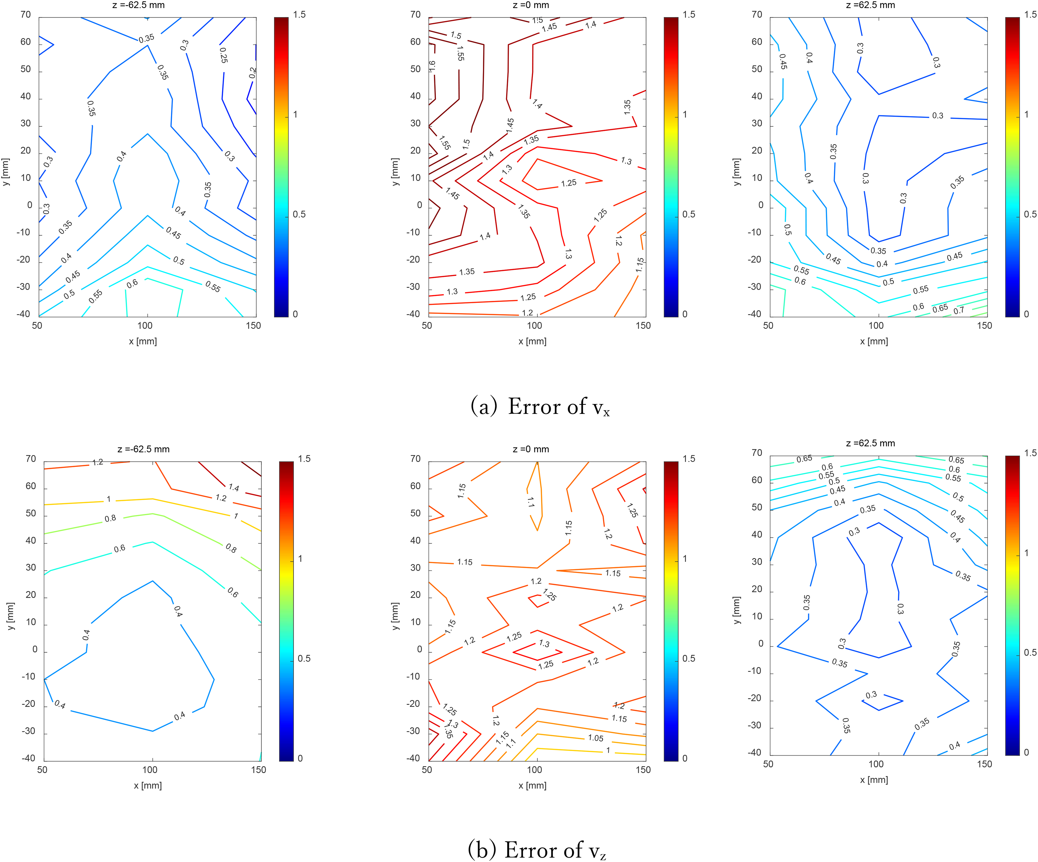
Distribution of wind speed modeling errors on the xy plane. (a) Error of v_x. (b) Error of v_z.

Figure 8.

Averaged modeling error of the x-y plane.

Figure 9 shows the measured and modeled wind speeds at (x,y,z) = (100, 0,0) and (100,0,-62.5). The position z = 0 was behind the vane. At z = -62.5, the measured wind speed histories are smooth compared to the ones behind the vane. The modeled wind speeds were in good agreement with the measured wind speeds. However, the measured wind speeds behind the vane oscillated at higher frequencies and did not agree with the modeled wind speeds.

Figure 9.

Comparison of modeled wind speeds and measured sample values. (a) v_x (x,y,z) = (100, 0, −62.5). (b) v_z (x,y,z) = (100, 0, −62.5). (c) v_x (x,y,z) = (100, 0, 0). (d) v_z (x,y,z) = (100, 0, 0).

Modeling errors were analyzed in the frequency region. The modeling error of the wind speed is defined as follows:

e_{x} = v_{z_{m o d e l}} - v_{x}

(9)

e_{z} = v_{z_{m o d e l}} - v_{z}

(10)

The power spectral densities (PSD) of the measured wind speeds and modeling errors were analyzed (Figures 10 and 11). The PSD of the wind speed at (x,y,z) = (100, 0, 0) when the vane was stationary at an angle of 0° was also plotted for comparison (Figure 12). The $f^{- 5 / 3}$ slope ( $f$ is the frequency) was plotted as a reference. In the frequency range with a slope of −5/3, the turbulent component was dominant in the inertial subrange.^34,35 In the frequency range where the slope is steeper than −5/3, turbulence is damped by viscosity. In the PSD of the static vane (Figure 12), strong peaks are observed at 72 Hz and higher frequencies, owing to a vortex generated from the trailing edge. In the frequency range above 72 Hz, the average slope is approximately −5/3, and turbulence is dominant. However, in the PSD, when the vane was moved (Figures 10 and 11), the peaks decreased. It can be assumed that the effect of the trailing edge vortex was reduced by the motion of the vane. The flow at z = -62.5 does not have a clear turbulent-dominated frequency band, and the power of flow above approximately 20 Hz is small. However, the flow behind the vane (z = 0) has a slope of −5/3 and is steeper in the frequency band above 72 Hz. The PSD of modeling errors shows that the flow behind the vane has large turbulence components compared to flow at z = -62.5 (Figure 11). It is assumed that the main component of the modeling error is high-frequency turbulence owing to the trailing-edge vortex of the vane. The wind speed model was valid at frequencies lower than the turbulence-dominant frequency.

Figure 10.

PSD of the measured wind speed. (a) vx (x,y,z) = (100, 0, −62.5). (b) vz (x,y,z) = (100, 0, −62.5). (c) vx (x,y,z) = (100, 0, 0). (d) vz (x,y,z) = (100, 0, 0).

Figure 11.

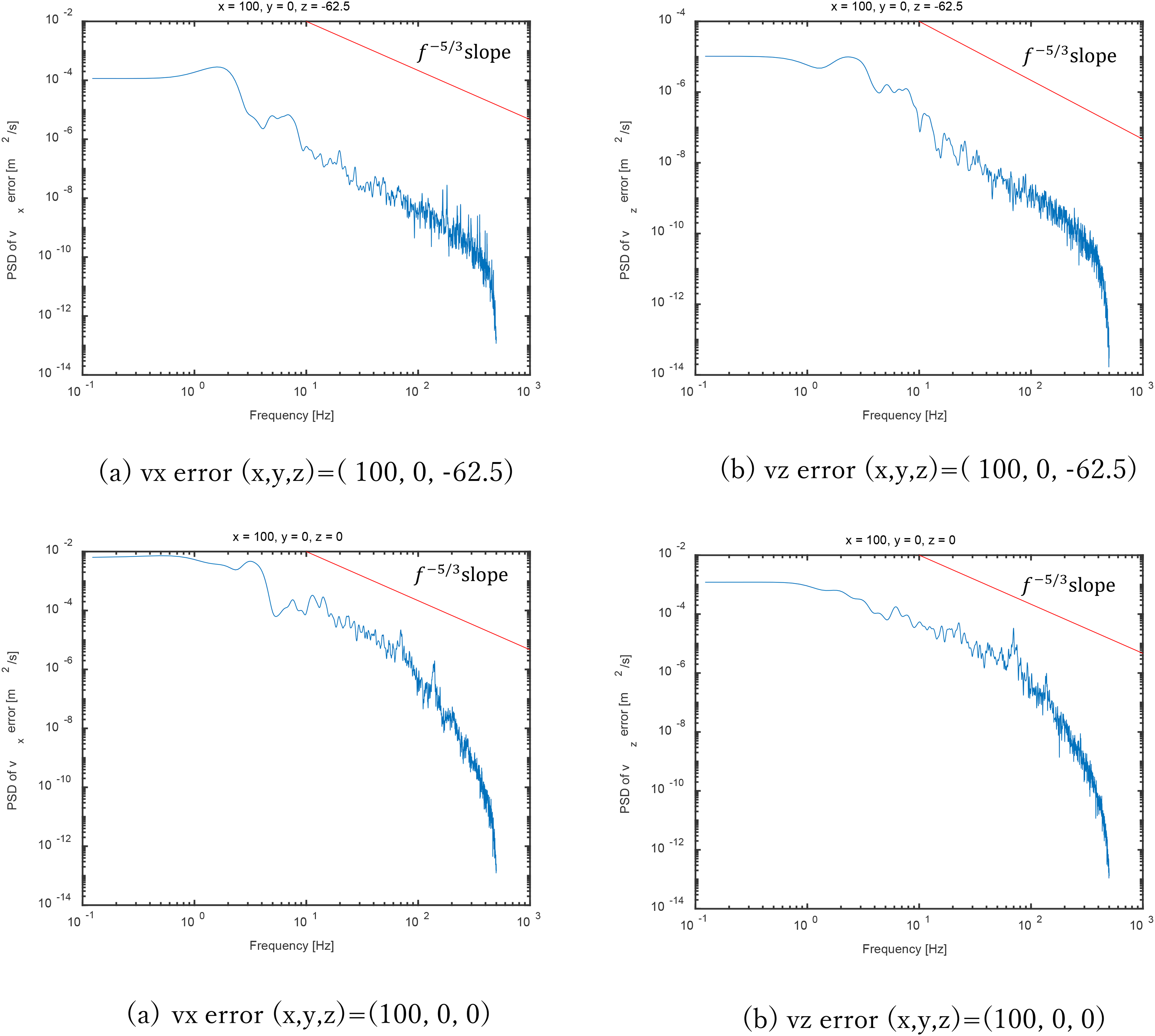
PSD of the modeling error of wind speed. (a) vx error (x,y,z) = (100, 0, −62.5). (b) vz error (x,y,z) = (100, 0, −62.5). (c) vx error (x,y,z) = (100, 0, 0). (d) vz error (x,y,z) = (100, 0, 0).

Figure 12.

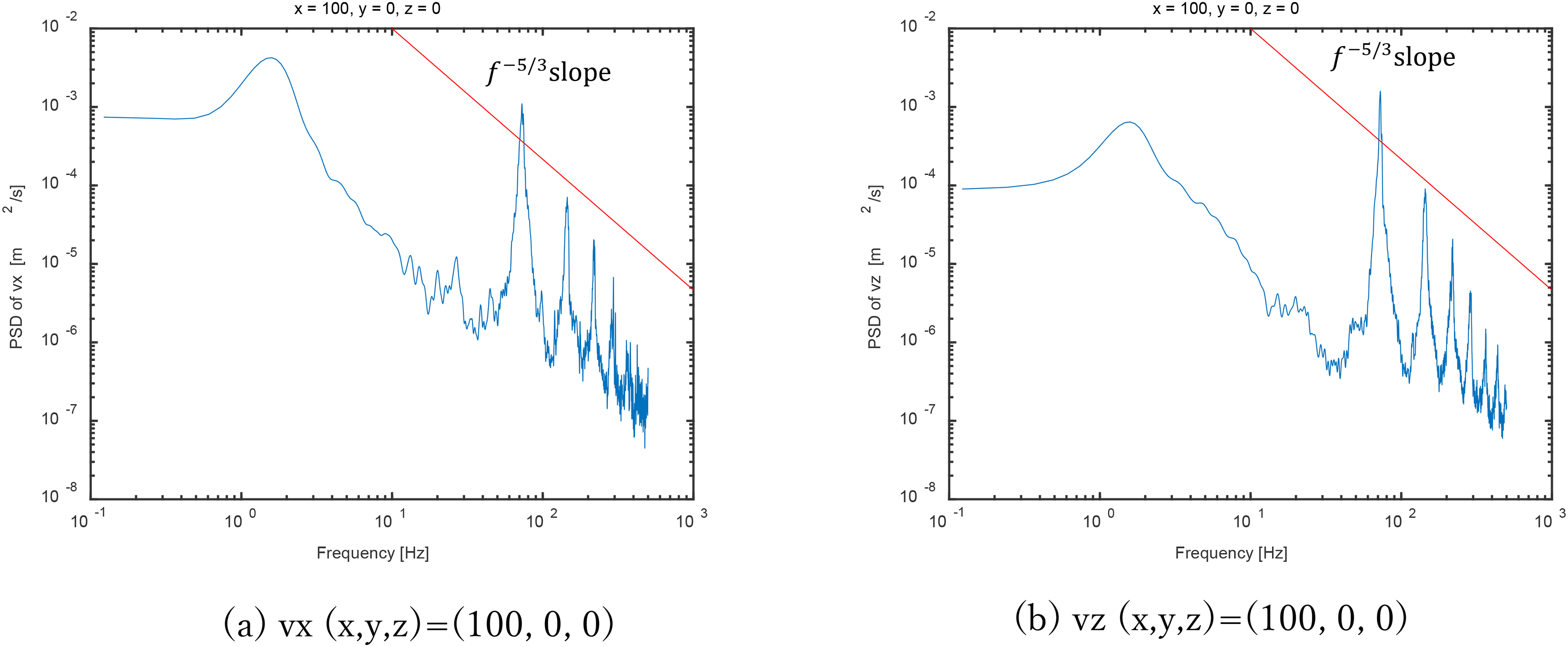
PSD of the measured wind speed (static vane). (a) vx (x,y,z) = (100, 0, 0). (b) vz (x,y,z) = (100, 0, 0).

Flight dynamics analysis of bumblebees using the wind tunnel

The oscillating wind histories in the test section were modeled, which can be applied to the dynamic identification of flying objects in a wind tunnel. Free-flight tests of bumblebees in gusts were conducted, and flight dynamics were identified and analyzed based on the captured videos.

Setup and position capture method

Figure 13 shows the experimental apparatus. Flight tests of bumblebees were conducted in the wind tunnel test section where wind modeling was performed. The sidewalls and ceiling were made of transparent plates. Flying bumblebees were filmed using two high-speed cameras (DITECT, HAS-D73), and their position and attitude were analyzed using motion capture software (DITECT, DIPP-MotionV). The frame rate was 500 fps, and the pixel count was 1280 × 1028.

Figure 13.

Experimental apparatus used for flight testing of bumblebee.

Flight experiments

The vane was moved by repeating the same 5 s history (Figure 2). A bumblebee is released into the test section of the wind tunnel and flies freely in the generated gust. The bumblebees used in the experiments were sourced from a commercial breeder (Agri Top Kuromaru Cube; Agrisect Inc., Ibaraki, Japan). Numerous flights were observed to crash owing to large changes in attitude caused by gusts. Figure 14 shows an example of a filmed flight. Figure 14(a) shows a stable flight in which the bumblebee flies forward without significant changes in attitude, while its attitude and position are affected by the gust. Figure 14(b) shows the bumblebee crashing to the ground on its back owing to a large pitch-up attitude caused by the gust. The gust encountered by bumblebees varies depending on their position and time of flight. These observations indicate that the flight control laws employed by bumblebees may not be sufficient to achieve a stable flight. Strategies for designing flight control laws for bumblebees were analyzed by identifying and analyzing stable flight dynamics. Two continuous stable flight datasets were obtained for the same bee (Flights 1 and 2). Flight 1 precedes Flight 2. Figure 15 shows the measured histories of the position and attitude. From the measured flight data, a dataset suitable for the precise identification of flight dynamics was extracted. In particular, the flight in the area with a modeling error of gust wind speed was smaller than almost 1% (Figures 7 and 8). From the extracted position history and gust wind model, Eq. (7), gust input histories along the ground-fixed axis were calculated. Figure 16 shows the gust input history of the bees. To eliminate the gust at high frequencies, a low-pass filter with a cutoff frequency of 50 Hz was applied to the measured data before the identification process.

Figure 14.

Typical bumblebee flights under gusty wind conditions. (a) Stable flight in gust wind. (b) Unstable flight in gust wind.

Figure 15.

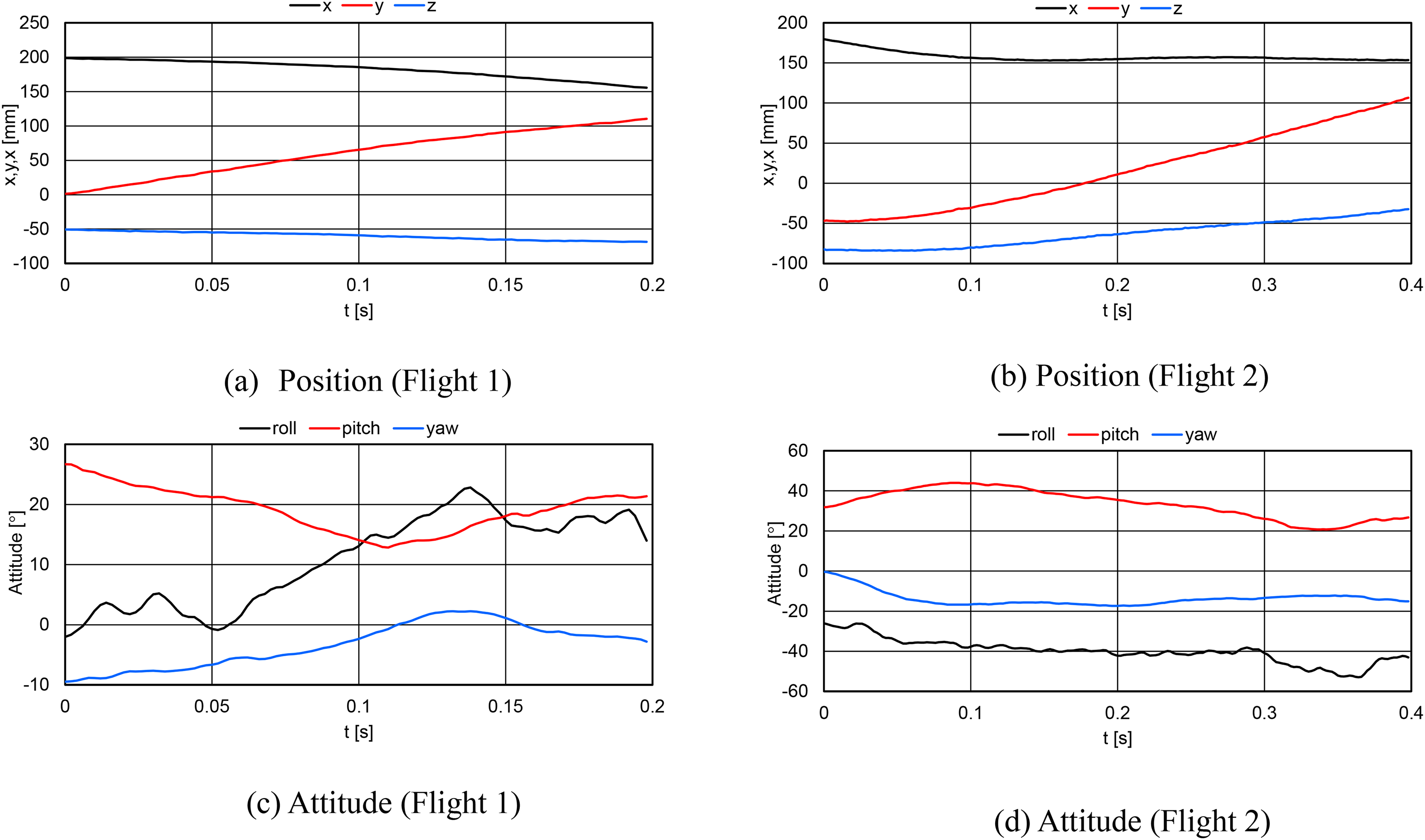
Position and attitude of flying bumblebee in gust wind . (a) Position (Flight 1). (b) Position (Flight 2). (c) Attitude (Flight 1). (d) Attitude (Flight 2).

Figure 16.

Gust input to the flying bumblebee. (a) Flight 1. (b) Flight 2.

Model identification

The observed attitude and position histories shown in Figure 15 are those of a successful flight, which is accomplished by the bee's flight control system that compensates for the gust response. This successful gust response history was modeled using a mathematical equation. The resulting model included bee-specific aerodynamics and feedback structure dynamics consisting of sensing, computation, and actuators. The precise modeling of a bee's flight requires a high-order linear or nonlinear model and a wide bandwidth for the disturbance input. However, the constructed disturbance wind tunnel generated a limited input frequency, enabling precise wind velocity modeling. Therefore, the dynamics of the bee for the bandwidth of the input disturbance are modeled with a low-order system.

The pitch angle and z-directional speed responses $θ$ and $\dot{z}$ to the gust inputs, $[v_{x} v_{z}]^{T}$ , which are important in longitudinal flight, are identified in the second-order, two-input, single-output state-space model. This can be equivalently expressed as a strictly proper second-order transfer function model with the same denominator coefficients.

θ (s) = \frac{b_{θ x 1} s + b_{θ x 0}}{s^{2} + a_{θ 1} s + a_{θ 0}} v_{x} (s) + \frac{b_{θ z 1} s + b_{θ z 0}}{s^{2} + a_{θ 1} s + a_{θ 0}} v_{z} (s)

(11)

\dot{z} (s) = \frac{b_{\dot{z} x 1} s + b_{\dot{z} x 0}}{s^{2} + a_{\dot{z} 1} s + a_{\dot{z} 0}} v_{x} (s) + \frac{b_{\dot{z} z 1} s + b_{\dot{z} z 0}}{s^{2} + a_{\dot{z} 1} s + a_{\dot{z} 0}} v_{z} (s)

(12)

Here, s denotes complex variable, and the coefficients of the rational polynomials are unknown parameters determined by optimization calculations.

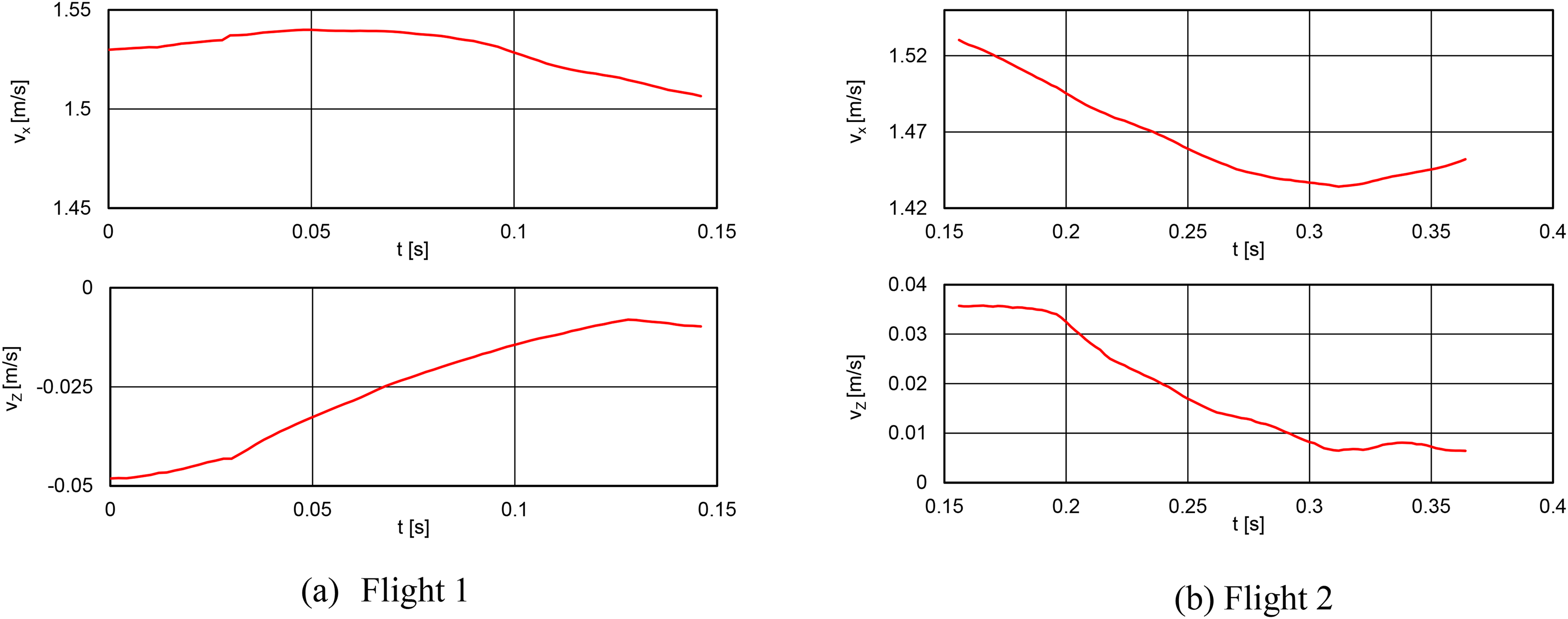
Figure 17 shows the power spectral density of the gust input. The generated gust contained frequency components up to 10 Hz. Therefore, the analysis of the flight dynamics of bees is reliable at this frequency. The deflection from the mean value was provided, and the second-order model was identified. Figure 18 shows the measured pitch angle and z-directional speed (downward positive) and the calculated outputs from the identified model. The measured values were offset such that the average value was zero. The response of Flight 1 was modeled with good accuracy. In Flight 2, the response at the same frequency as that in Flight 1 was modeled with good accuracy. However, it is not possible to model high-frequency oscillations.

Figure 17.

PSD of the gust input to flying bumblebee. (a) Flight 1. (b) Flight 2.

Figure 18.

Measured responses and model output of flying bumblebee in gust wind. (a) Flight 1. (b) Flight 2.

The preciseness of the identified model is evaluated by output error as follows:

J_{#} = \frac{{‖ #_{m o d e l} (t) - # (t) ‖}_{p}}{{‖ # (t) ‖}_{p}} \times 100, # : θ, {\dot{z}}_{E}

(13)

here,

θ and {\dot{z}}_{E}

denote the measured angle of the attack, which is the longitudinal angle of bees relative to wind speed vector and the ze-directional speed, respectively.

#_{m o d e l}

denotes the calculated output from identified models. The evaluated modeling errors in Table 2 also indicate that Flight 2 is less accurate.

Table 2.

Identification errors in the gust response model.

	Flight 1	Flight 2
$J_{θ}$	8.97%	27.8%
$J_{{\dot{z}}_{E}}$	10.5%	29.8%

Analysis of control strategy

The identified model should represent the response resulting from tuning the control system for certain purposes. In the design of control systems for artificial objects, the loop-shaping method³⁶ is often used to suppress the disturbance response. Because the identified model has two inputs, the frequency responses of the largest singular value of $G_{θ} (j ω)$ and $G_{\dot{z}} (j ω)$ , which are the identified transfer functions with an output of pitch angle and z-directional speed and gust input ${[\begin{matrix} v_{x} & v_{z} \end{matrix}]}^{T}$ are plotted (Figure 19). Both the pitch angle and velocity output gains were smaller for Flight 1 than for Flight 2 at low frequencies but larger at high frequencies. A frequency band with a small disturbance response indicates that a large feedback gain was provided. In the large feedback gain frequency band, the sensitivity function decreases, and the tracking performance improves. The smoothness of the measured history of Flight 1 compared with that of Flight 2 suggests successful disturbance suppression and tracking. Flight 2 has a larger disturbance response owing to the use of smaller feedback gains in the low-frequency range. However, highly robust stability against model uncertainties, such as variations in the aerodynamic properties of a flapping wing in a continuously fluctuating gust wind, can be attained. This bumblebee was selected for high robust stability at the expense of disturbance suppression after a flight with good disturbance suppression. Thus, it can be inferred that the control system was adapted using this strategy.

Figure 19.

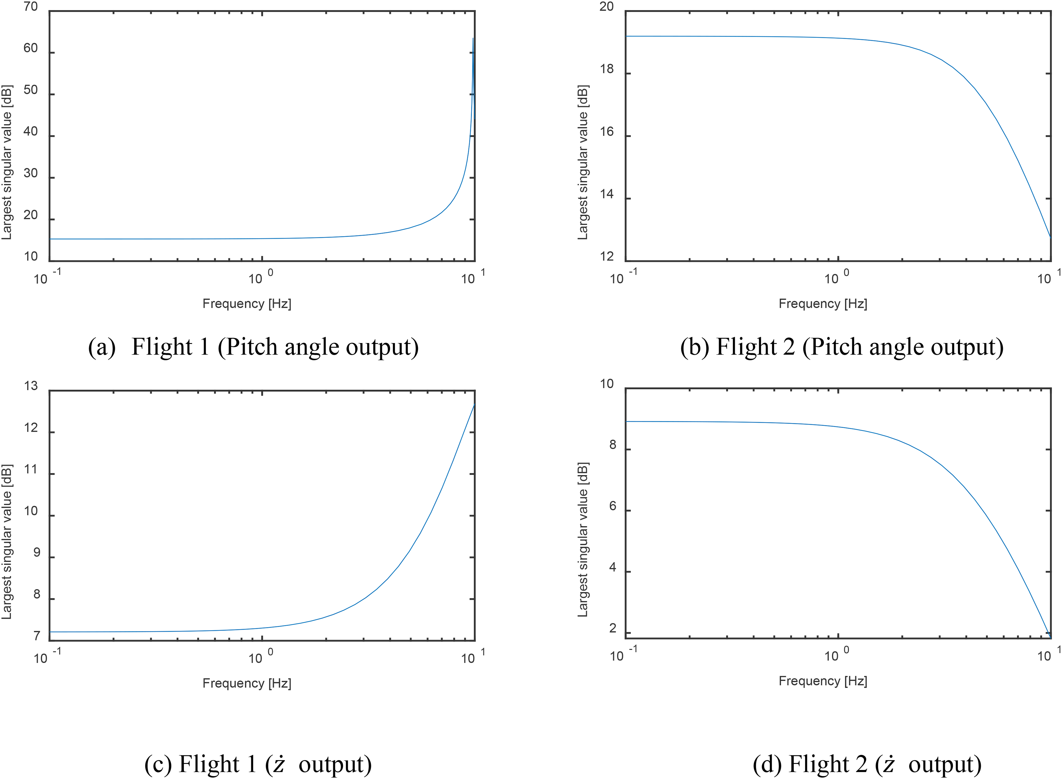
Frequency responses of disturbance responses gust response model of bumblebee. (a) Flight 1 (Pitch angle output). (b) Flight 2 (Pitch angle output). (c) Flight 1 ( $\dot{z}$ output). (d) Flight 2 ( $\dot{z}$ output).

Conclusions

A turbulent wind tunnel was developed to identify the motion of free-flying objects. Oscillating vanes were installed upstream of the test section to measure the wind velocity distribution in the test section and its temporal variations. The wind velocity distribution in the wind tunnel was modeled using the measured data to obtain the wind speed and direction encountered by the flying object from the position and time of the object. Except for the downstream of the vanes, the modeling error for wind speed was less than 1%. A flight test of a free-flying bumblebee in a continuous gust was conducted, and the gust response transfer function of the bee was identified based on the measured position and attitude and the established wind distribution model. It was found that, depending on the flight, the bee adapts by selecting a large feedback gain that suppresses the gust response or a small gain that improves robust stability. The inference for the bee control system design strategy was based on the identified models of the two flights. Further experiments with various disturbances may reveal more detailed adaptation policies and learning processes among bees. The developed experimental setup can also be extended to investigate the dynamics of MAVs under turbulent conditions. Moreover, the bee dynamics model, derived through multiple unstable flight attempts, can inform adaptive flight control strategies in MAVs to improve their robustness against wind disturbances.

Footnotes

ORCID iDs

Hiroshi Tokutake

Hikaru Otsuka

Funding

The authors disclosed receipt of the following financial support for the research, authorship, and/or publication of this article: This work was supported by JSPS KAKENHI (grant number 23K17320).

Declaration of conflicting interests

The authors declared no potential conflicts of interest with respect to the research, authorship, and/or publication of this article.

References

Thielicke

Kesel

Stamhuis

. Reliable force predictions for a flapping-wing micro air vehicle: a “vortex-lift” approach. Int J Micro Air Veh 2011; 3: 201–215.

Reid

Zhou

Maxcer

, et al. Toward the design of dynamically similar artificial insect wings. Int J Micro Air Veh 2021; 13.

Sims

Palazotto

Norris

. A structural dynamic analysis of a manduca sexta forewing. Int J Micro Air Veh 2010; 2: 119–140.

Taylor

Thomas

ALR

. Dynamic flight stability in the desert locust Schistocerca gregaria. J Exp Biol 2003; 206: 2803–2829.

Sun

Xiong

. Dynamic flight stability of a hovering bumblebee. J Exp Biol 2005; 208: 447–459.

Karásek

Hua

Nan

, et al. Pitch and roll control mechanism for a hovering flapping wing MAV. Int J Micro Air Veh 2014; 6: 253–264.

Phan

Aurecianus

Kang

, et al. KUBeetle-S: An insect-like, tailless, hover-capable robot that can fly with a low-torque control mechanism. Int J Micro Air Veh 2019; 11.

Tubbs

Palazotto

Willis

. Biological investigation of wing motion of the manduca sexta. Int J Micro Air Veh 2011; 3: 101–117.

Koopmans

Tijmons

De Wagter

, et al. Passively stable flapping flight from Hover to fast forward through shift in wing position. Int J Micro Air Veh 2015; 7: 407–418.

10.

De Clercq

KME

de Kat

Remes

, et al. Aerodynamic experiments on DelFly II: unsteady lift enhancement. Int J Micro Air Veh 2009; 1: 255–262.

11.

de Croon

GCHE

de Clercq

KME

Ruijsink

, et al. Design, aerodynamics, and vision-based control of the DelFly. Int J Micro Air Veh 2009; 1: 71–97.

12.

De Wagter

Koopmans

de Croon

, et al. Autonomous wind tunnel free-flight of a flapping wing MAV. In: Advances in aerospace guidance, navigation and control. Berlin, Heidelberg: Springer Berlin Heidelberg, 2013, pp.603–621.

13.

Phan

Kang

Park

. Design and stable flight of a 21g insect-like tailless flapping wing micro air vehicle with angular rates feedback control. Bioinspir Biomim 2017; 12: 036006.

14.

Karásek

Hua

Nan

, et al. Pitch and roll control mechanism for a hovering flapping wing MAV. Int JMicro Air Veh 2014; 6: 253–264.

15.

Pérez-Arancibia

Galloway

, et al. First controlled vertical flight of a biologically inspired microrobot. Bioinspir Biomim 2011; 6: 036009.

16.

Keennon

Klingebiel

Won

. Development of the nano hummingbird: a tailless flapping wing micro air vehicle. In: 50th AIAA Aerospace Sciences Meeting including the New Horizons Forum and Aerospace Exposition. Reston, Virigina: American Institute of Aeronautics and Astronautics, 2012; AIAA 2012-0588.

17.

Karásek

Muijres

De Wagter

, et al. A tailless aerial robotic flapper reveals that flies use torque coupling in rapid banked turns. Science (1979) 2018; 361: 1089–1094.

18.

Sheng

Liu

, et al. Experimental study on the aerodynamic optimization design of flexible wings for tailless flapping wing micro air vehicles. Int J Micro Air Veh 2025; 17.

19.

Zhang

Wang

. An experimental study of the unsteady vortex structures of a clapping-wing micro air vehicle. Int J Micro Air Veh 2022; 14.

20.

Runco

Benedict

. Flight dynamics model identification of a meso-scale twin-cyclocopter in hover. Int J Micro Air Veh 2023; 15.

21.

Runco

Benedict

. Design, development, and flight testing of a 70-gram micro quad-cyclocopter. Int J Micro Air Veh 2023; 15.

22.

Jakobi

Kolomenskiy

Ikeda

, et al. Bees with attitude: the effects of directed gusts on flight trajectories. Biol Open 2018; 7: 1–10.

23.

Matthews

Sponberg

. Hawkmoth flight in the unsteady wakes of flowers. J Exp Biol 2018; 221: jeb179259.

24.

Burnett

Badger

Combes

. Wind and obstacle motion affect honeybee flight strategies in cluttered environments. J Exp Biol 2020; 223: jeb222471.

25.

Nakata

Noda

Kumagai

, et al. A simulation-based study on longitudinal gust response of flexible flapping wings. Acta Mech Sin 2018; 34: 1048–1060.

26.

Tanaka

Kawachi

. Response characteristics of visual altitude control system in Bombus terrestris. J Exp Biol 2006; 209: 4533–4545.

27.

Dickinson

Lighton

JRB

. Muscle efficiency and elastic storage in the flight motor of Drosophila. Science (1979) 1995; 268: 87–90.

28.

Lawson

KKK

Srinivasan

. Flight control of fruit flies: dynamic response to optic-flow and headwind. J Exp Biol 2017; 220: 2005–2016.

29.

Balatti

Khodaparast

Friswell

, et al. Improving wind tunnel “1-cos” gust profiles. J Aircr 2022; 59: 1514–1528.

30.

Hamada

Saitoh

Kobiki

. Gust alleviation control using prior gust information: Wind tunnel test results. IFAC-PapersOnLine 2019; 52: 128–133.

31.

Kobayashi

Hatanaka

. Active generation of wind gust in a two-dimensional wind tunnel. J Wind Eng Ind Aerodyn 1992; 42: 959–970.

32.

Hart

Sytsma

Ukeiley

. An aerodynamic characterization facility for micro air vehicle research. Int J Micro Air Veh 2016; 8: 79–91.

33.

David

. Spectral feedback control of turbulent spectra in a wind tunnel. Exp Fluids 2020; 61: 175.

34.

Kolmogorov

. The local structure of turbulence in incompressible viscous fluid for very large reynolds numbers. Dokl Akad Nauk SSSR 1941; 30: 301–304.

35.

Champagne

. The fine-scale structure of the turbulent velocity field. J Fluid Mech 1978; 86: 67–108.

36.

Zhou

Doyle

Glover

. Robust and optimal control. Upper Saddle River: Prentice Hall, 1996.

Design of a gust-generating wind tunnel for dynamic identification of micro air vehicles and bumblebee flight

Abstract

Keywords

Introduction

Development of the wind tunnel with gust generator

Gust generator

Wind speed distribution

Wind gust model

Flight dynamics analysis of bumblebees using the wind tunnel

Setup and position capture method

Flight experiments

Model identification

Analysis of control strategy

Conclusions

Footnotes

ORCID iDs

Funding

Declaration of conflicting interests

References