Improved moving horizon estimation for ultra-wideband localization on small drones

Abstract

Moving Horizon Estimation (MHE) offers multiple advantages over Kalman Filters when it comes to the localization of drones. However, due to the high computational cost, they can not be used on Micro Air Vehicles (MAVs) with limited computational power. We have previously shown, that with a few assumptions and simplifications, MHE can be made more efficient while retaining good localization performance. In this paper, we present two additional improvements: the introduction of dynamic step sizes to the gradient descent algorithm, which leads to a significant increase in robustness, and the use of switching variables for outlier rejection, which further reduces the computational load. Both improvements are implemented and assessed in simulation and experiments. Using dynamic step sizes makes it possible to reliably use the estimator on board a real drone, and the use of Newton’s method specifically opens the option to add different types of measurements. The new outlier rejection method on the other hand is shown to reduce the computational load significantly without impacting the accuracy.

Introduction

Self-localization is an important task for autonomous drones, especially when operating in indoor environments. ¹ Since navigation using Global Navigation Satellite Systems (GNSS) exhibits a significant decrease in performance when used inside buildings, other solutions are needed. Ultra-wideband (UWB) technology has been investigated as a promising alternative in scenarios where the environment can be prepared in advance.^2–4 UWB localization works in a similar fashion as GNSS, but instead of ranging with respect to satellites, it uses fixed beacons at known locations in the environment. ⁵

The UWB range measurements can be used for triangulation, ⁶ but are more commonly fused with measurements from an inertial measurement unit (IMU) for more accurate results. ³ Kalman filter variants such as the Extended Kalman Filter (EKF) are often used due to their speed and efficiency. ⁷ However, they are not ideal when working with highly non-linear dynamics or non-Gaussian noise, both of which are present in the system in question. ⁸

Moving Horizon Estimators (MHEs) are better suited for state estimation in non-linear systems with non-Gaussian noise, ⁹ but are computationally expensive, which makes them impractical to use on small drones with limited computational power. In our previous work, we investigated several simplifications that reduce the load for localization of small drones using an MHE. ⁸ While the resulting estimator performed well in offline evaluations on real measurement data, its robustness was found to be lacking. Specifically in situations where the number of incoming measurements varies a lot, the tuning had to be quite conservative to avoid unstable behaviour when many measurements were coming in. Furthermore, while we were happy with the performance of Random Sample Consensus (RANSAC) for outlier rejection, its computational cost was quite high for an algorithm aimed at computationally extremely limited systems, like the micro-controllers on board of nano-drones.

In this paper, we will present the following two improvements to efficient moving horizon estimation for localization with UWB:

Using a dynamic step size in the gradient-descent step to improve robustness

Outlier rejection based on switching variables to further improve the computational efficiency

Preliminaries

Computationally efficient MHE

Let us quickly review the computationally efficient MHE presented in Pfeiffer et al. ⁸ to highlight some of its shortfalls. We again consider the discrete-time non-linear dynamic system given by (1), expressed in terms of the system state $\mathit{\xi }$ , input vector $\mathit{u}$ , measurement vector $\mathit{y}$ , process noise $\mathit{w}$ and measurement noise $\mathit{v}$ , all at timestep $t$ respectively.

$$\{\begin{array}{cc}{\mathit{\xi }}_{t+1}& =\mathit{f}({\mathit{\xi }}_t,{\mathit{u}}_t)+{\mathit{w}}_t\\ {\mathit{y}}_t& =\mathit{h}({\mathit{\xi }}_t,{\mathit{u}}_t)+{\mathit{v}}_t\end{array}$$

(1)

The full MHE problem for a horizon of length $N+1$ is given by the optimization problem (2), formulated in terms of the decision variables $\mathit{\xi }$ , $\mathit{w}$ and $\mathit{v}$ . Put into words, the MHE tries to minimize the squared observed process and measurement noise, as well as changes to the prior estimate (also called the arrival cost). The prior ${\overline{\xi }}_{t-N}$ is calculated from the previous estimate using the prediction equation, ${\overline{\xi }}_{t-N}=\mathit{f}({\hat{\xi }}_{t-N-1})$ .

$$\begin{array}{c}\underset{\mathit{\xi },\mathit{w},\mathit{v}}{min}\mu \Vert {\mathit{\xi }}_{t-N}-{\overline{\xi }}_{t-N}{\Vert }^2+\sum _{k=t-N}^{t-1}{\mathit{w}}_k^2+\sum _{k=t-N}^t{\mathit{v}}_k^2\\ \text{s.t.}{\mathit{\xi }}_{k+1}=\mathit{f}({\mathit{\xi }}_k,{\mathit{u}}_k)+{\mathit{w}}_k\\ {\mathit{y}}_k=\mathit{h}({\mathit{\xi }}_k,{\mathit{u}}_k)+{\mathit{v}}_k\end{array}$$

(2)

By assuming negligible process noise ( $\mathit{w}=\mathbf{0}$ ), the problem can be reduced to an output error MHE. Furthermore, by defining the composite prediction and measurement equations ${\mathcal{F}}_k({\mathit{\xi }}_{t-N})$ and ${\mathcal{H}}_{i,k}({\mathit{\xi }}_{t-N})$ , we can merge the constraints into the cost-function $J$ , which now only depends on the decision variable ${\mathit{\xi }}_{t-N}$ . Note that the number of measurements $m_t$ can differ between timesteps.

$${\mathcal{F}}_k({\mathit{\xi }}_{t-N})={\mathit{f}}^{u_k}\circ \dots \circ {\mathit{f}}^{u_{t-N}}({\mathit{\xi }}_{t-N})$$

(3)

$${\mathcal{H}}_{i,k}({\mathit{\xi }}_{t-N})=h_i^{u_k}\circ {\mathcal{F}}_{k-1}({\mathit{\xi }}_{t-N})$$

(4)

$$\begin{array}{rl}J({\mathit{\xi }}_{t-N})=& \mu \Vert {\mathit{\xi }}_{t-N}-{\overline{\xi }}_{t-N}{\Vert }^2\\ & +\sum _{k=t-N}^t\sum _{i=1}^{m_t}(\Vert y_{i,k}-{\mathcal{H}}_{i,k}({\mathit{\xi }}_{t-N}){\Vert }^2)\end{array}$$

(5)

To save computation time, instead of fully solving the optimization problem at every timestep, only a single gradient descent step is performed as suggested by Alessandri and Gaggero. ¹⁰

$${\hat{\xi }}_{t-N}={\overline{\xi }}_{t-N}-\alpha \mathrm{\nabla }J({\overline{\xi }}_{t-N})$$

(6)

Using the chain rule, the gradient of the cost function is easily calculated analytically. When using only a single iteration, the gradient is calculated with the prior best estimate ${\mathit{\xi }}_{t-N}={\overline{\xi }}_{t-N}$ , thus the arrival cost term is zero.

$$\mathrm{\nabla }J({\overline{\xi }}_{t-N})=-2\sum _{k=t-N}^t\sum _{i=1}^{m_t}[(y_{i,k}-{\mathcal{H}}_{i,k}({\overline{\xi }}_{t-N}))\mathrm{\nabla }{\mathcal{H}}_{i,k}({\overline{\xi }}_{t-N})]$$

(7)

To save computational power, the gradient of the composite measurement equation can be simplified by iterative computation of the Jacobian of the composite prediction equation (chain rule):

$$\mathrm{\nabla }{\mathcal{H}}_{i,k}({\overline{\xi }}_{t-N})={(\mathrm{D}{\mathcal{F}}_{k-1}({\overline{\xi }}_{t-N}))}^T\cdot \mathrm{\nabla }{h}_i({\overline{\xi }}_k,{\mathit{u}}_k)$$

(8)

$$\mathrm{D}{\mathcal{F}}_{k-1}({\overline{\xi }}_{t-N})=\mathrm{D}\mathit{f}({\overline{\xi }}_{k-1},{\mathit{u}}_{k-1})\cdot \mathrm{D}{\mathcal{F}}_{k-2}({\overline{\xi }}_{t-N})$$

(9)

For outlier rejection, a RANSAC scheme was used, which can identify outliers very well but requires a significant amount of computational power.

Drone and measurement model

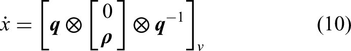
We use the drone model in Mueller et al., ³ but represent the attitude in quaternions and simplify the drag forces. For the use in our estimator, we discretize the model using the forward Euler method.

$$\dot{x}={[\mathit{q}\otimes \left[\begin{array}{c}0\\ \mathit{\rho }\end{array}\right]\otimes {\mathit{q}}^{-1}]}_v$$

(10)

$$\dot{\rho }=\frac{f}{m}{\mathit{e}}_{\mathbf{3}}+({\mathbf{K}}_a-[[{\mathit{\omega }}_{\times }]])\mathit{\rho }-{[{\mathit{q}}^{-1}\otimes \left[\begin{array}{c}0\\ \mathit{g}\end{array}\right]\otimes \mathit{q}]}_v$$

(11)The six dimensional state vector $\mathit{\xi }=[{\mathit{x}}^T,{\mathit{\rho }}^T{]}^T$ contains the position $\mathit{x}\in {\mathbb{R}}^3$ in the global frame and the drone’s velocities $\mathit{\rho }\in {\mathbb{R}}^3$ in the body frame. The system inputs are the total thrust $f$ , the attitude quaternion $\mathit{q}\in {\mathbb{R}}^4$ , and the angular velocities measured by the IMU, $\mathit{\omega }\in {\mathbb{R}}^3$ . $m$ is the drone’s mass and ${\mathbf{K}}_{\text{a}}=\text{diag}(k_{\perp },k_{\perp },k_{\Vert })$ are the linear drag coefficients. The quaternion product is noted as $\otimes$ , while the subscript $0$ and $v$ refer to the scalar and vector portion of the quaternion respectively. Finally, $\mathit{g}$ is the acceleration due to gravity and $[[{\mathit{\omega }}_{\times }]]$ is the skew-symmetric matrix defined as

$$[[{\mathit{\omega }}_{\times }]]=\left[\begin{array}{ccc}0& -{\omega }_3& {\omega }_2\\ {\omega }_3& 0& -{\omega }_1\\ -{\omega }_2& {\omega }_1& 0\end{array}\right]$$

(12)

We consider two different types of UWB measurements. Two-way ranging (TWR) can be used to determine the distance between the drone and a fixed beacon located at ${\mathit{p}}_A$ . Time-difference of Arrival (TDOA) measurements on the other hand represent the difference in the distance of the drone to two fixed beacons at positions ${\mathit{p}}_A$ and ${\mathit{p}}_B$ . The measurement noise is represented by ${\eta }_{\text{twr}}$ and ${\eta }_{\text{TDOA}}$ respectively.

$$y_{\text{twr}}=\Vert {\mathit{p}}_A-\mathit{x}\Vert +{\eta }_{\text{twr}}$$

(13)

$$y_{\text{TDOA}}=\Vert {\mathit{p}}_A-\mathit{x}\Vert -\Vert {\mathit{p}}_B-\mathit{x}\Vert +{\eta }_{\text{TDOA}}$$

(14)

Dynamic step size

A serious problem with the approach in Pfeiffer et al. ⁸ is the fixed step size used in the gradient descent algorithm. Specifically in situations where the number of measurements $m_t$ varies between steps, the fact that the gradient of the cost function is the sum of $m_t$ individual measurement terms can lead to large variations in the gradient’s magnitude. As a result, a value for $\alpha$ that is optimal with 4 UWB beacons, might cause the estimator to become unstable for 8 beacons. A solution to this problem is to dynamically adjust the step size of the gradient descent algorithm. We investigated two options for choosing the step size dynamically: linesearch and Newton’s method. While robustness is of course an important property of any state estimation algorithm, it should be noted that we are sacrificing computational efficiency to achieve it.

Linesearch

With the linesearch method, different values for the step size $\alpha$ are tested at each time step. The step size resulting in the estimate with the lowest cost is then retained for the next step. The algorithm is laid out in Algorithm 1.

Algorithm 1

Linesearch Method

$t\leftarrow 0\mathit{\xi }\leftarrow {\mathit{\xi }}_0\alpha \leftarrow {\alpha }_0$ $s\leftarrow \{0.5,0.8,1.0,1.25,2.0\}$ while running do     $t\leftarrow t+1$    calculate $\mathrm{\nabla }J({\mathit{\xi }}_{t-N})$    for $s_i\in s$ do        ${\mathit{\xi }}_i={\mathit{\xi }}_{t-N}-s_i\cdot \alpha \mathrm{\nabla }J({\mathit{\xi }}_{t-N})$       calculate $J_i({\mathit{\xi }}_i)$    end for     $i_{\text{opt}}\leftarrow {\mathrm{argmin}}_i(J_i)$     ${\mathit{\xi }}_{t-N}\leftarrow {\mathit{\xi }}_{i_{\text{opt}}}$     $\alpha \leftarrow s_{i_{\text{opt}}}\cdot \alpha$ end while

The linesearch method is easy to implement in the existing algorithm but has the downside of scaling the step size for all state variables at once. If different types of measurements are available, this can lead to problems. As an example, if a lot of velocity estimates are available but only a few position estimates, it would be good to choose different step sizes for the different states. An approach that allows for this flexibility is the use of Newton’s method.

Newton’s method

Newton’s method is more complex to implement than linesearch, but offers two additional advantages. First, there is no need to calculate the cost of multiple estimates (which requires several predictions through the complete horizon) and second, Newton’s method allows to adjust the step size along different axes. Specifically, instead of using a scalar step size $\alpha$ , the gradient of the cost function is multiplied by the inverse Hessian matrix of the cost function:

$${\hat{\xi }}_{t-N}={\overline{\xi }}_{t-N}-{({\mathrm{D}}^{2}J({\overline{\xi }}_{t-N}))}^{-1}\mathrm{\nabla }J({\overline{\xi }}_{t-N})$$

(15)

The Hessian matrix of the cost function can be obtained by calculating the Jacobian of the cost function gradient.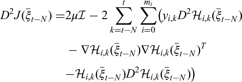

$$\begin{array}{rl}{\mathrm{D}}^{2}J({\overline{\xi }}_{t-N})=& 2\mu \mathcal{I}-2\sum _{k=t-N}^t\sum _{i=0}^{m_t}(y_{i,k}{\mathrm{D}}^2{\mathcal{H}}_{i,k}({\overline{\xi }}_{t-N})\\ & -\mathrm{\nabla }{\mathcal{H}}_{i,k}({\overline{\xi }}_{t-N})\mathrm{\nabla }{\mathcal{H}}_{i,k}({\overline{\xi }}_{t-N}{)}^T\\ & -{\mathcal{H}}_{i,k}({\overline{\xi }}_{t-N}){\mathrm{D}}^2{\mathcal{H}}_{i,k}({\overline{\xi }}_{t-N}))\end{array}$$

(16)

As with the gradients, the Hessian matrices of the cost and measurement functions can be calculated algebraically in an iterative manner while stepping through the horizon. Making use of the chain rule, we find the following expression: ¹¹

$$\begin{array}{rl}{\mathrm{D}}^2{\mathcal{H}}_{i,k}(\mathit{\xi })=& {(\mathrm{D}{\mathcal{F}}_{k-1}(\mathit{\xi }))}^T\cdot {\mathrm{D}}^{2}h({\mathcal{F}}_{k-1}(\mathit{\xi }))\cdot \mathrm{D}{\mathcal{F}}_{k-1}(\mathit{\xi })\\ & +\sum _{j=1}^n\frac{\mathrm{\partial }h}{\mathrm{\partial }{\xi }_j}({\mathcal{F}}_{k-1}(\mathit{\xi }))\cdot {\mathrm{D}}^2{\mathcal{F}}_{k-1}^j(\mathit{\xi })\end{array}$$

(17)

Luckily, many of the terms appearing in this equation are already needed when calculating the cost function gradient. Furthermore, since the prediction model we use is linear in terms of the states, the Hessian matrix of the composite prediction equations turns out to be zero. The simplified expression for the Hessian matrix of the cost function thus only depends on the Hessian matrix of the measurement function and the Jacobian matrix of the composite prediction equation:

$${\mathrm{D}}^2{\mathcal{H}}_{i,k}(\mathit{\xi })=(\mathrm{D}{\mathcal{F}}_{k-1}(\mathit{\xi }){)}^T\cdot {\mathrm{D}}^{2}h({\mathcal{F}}_{k-1}(\mathit{\xi }))\cdot \mathrm{D}{\mathcal{F}}_{k-1}(\mathit{\xi })$$

(18)

Switching variable outlier rejection

Since using RANSAC for outlier rejection has the disadvantage of being computationally heavy, we decided to look for a more efficient method. The need for outlier rejection in optimization problems also arises in Simultaneous Localization and Mapping (SLAM), where incorrectly identified loop-closures can cause large errors in the resulting map. A possible approach to deal with this issue is the addition of switching variables that multiply the constraints in question. ¹² Applying this concept to our MHE, we introduce for each measurement $y_{i,k}$ an associated switching variable $s_{i,k}$ . By giving the optimization algorithm the ability to change these switching variables, the algorithm can enable and disable measurements based on how they impact the value of the cost function.

To use the switching variables as decision variables, they must be continuous. At the same time, for their function to enable and disable measurements, binary values would be more useful. Following Sünderhauf and Protzel, ¹² we use a sigmoid function to convert the continuous switching variables into values between 0 and 1, which then multiply the measurement equation. A simple sigmoid function to use is the logistic function (19).

$$\mathrm{sig}(s_{i,k})=\frac{1}{1+e^{-s_{i,k}}}$$

(19)

In the context of calculating gradients, it is also helpful to note the derivative of the logistic function (20).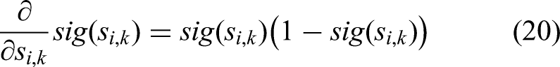

$$\frac{\mathrm{\partial }}{\mathrm{\partial }{s}_{i,k}}\mathrm{sig}(s_{i,k})=\mathrm{sig}(s_{i,k})(1-\mathrm{sig}(s_{i,k}))$$

(20)

It is important to penalize the estimator for ignoring a measurement. We do this by adding a term similar to the arrival cost, that penalizes switching variables that deviate from a prior value $\overline{s}$ , which enables the measurement (e.g. $\overline{s}=5$ ). To simplify notation, we collect all switching variables in a single column vector $\mathit{s}=[s_{i,j}]$ . The resulting cost function including switching variables then looks like this:

$$\begin{array}{rl}J({\mathit{\xi }}_{t-N},\mathit{s})=& \mu {\Vert {\mathit{\xi }}_{t-N}-{\overline{\xi }}_{t-N}\Vert }^2\\ & +{\mu }_s\cdot \sum _{k=t-N}^t\sum _{i=1}^m{(s_{i,k}-\overline{s})}^2\\ & +\sum _{k=t-N}^t\sum _{i=1}^m(\mathrm{sig}(s_{i,k})\cdot {\Vert y_{i,k}-{\mathcal{H}}_{i,k}({\mathit{\xi }}_{t-N})\Vert }^2)\end{array}$$

(21)

When calculating the gradient of the cost function, we now also need to consider the derivative with respect to the individual switching variables. Luckily, each switching variable only appears once in each of the two sums and the corresponding derivative is easily calculated:

$$\begin{array}{rl}\frac{\mathrm{\partial }J}{\mathrm{\partial }{s}_{i,k}}({\mathit{\xi }}_{t-N},\mathit{s})=& 2{\mu }_s(s_{i,k}-\overline{s})\\ & +\mathrm{sig}(s_{i,k})(1-\mathrm{sig}(s_{i,k}))\cdot \\ & {\Vert y_{i,k}-{\mathcal{H}}_{i,k}({\mathit{\xi }}_{t-N})\Vert }^2\end{array}$$

(22)

The changes to the derivatives with respect to 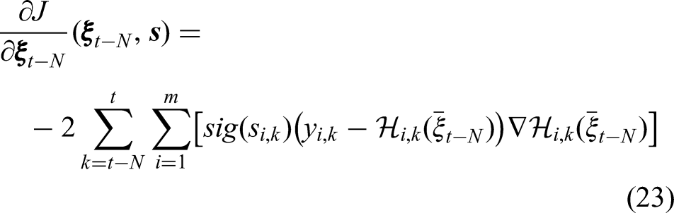${\mathit{\xi }}_{t-N}$ are also small, one only has to add the sigmoid multiplication to each of the terms of the sums:

$$\begin{array}{rl}& \frac{\mathrm{\partial }J}{\mathrm{\partial }{\mathit{\xi }}_{t-N}}({\mathit{\xi }}_{t-N},\mathit{s})=\\ & -2\sum _{k=t-N}^t\sum _{i=1}^m[\mathrm{sig}(s_{i,k})(y_{i,k}-{\mathcal{H}}_{i,k}({\overline{\xi }}_{t-N}))\mathrm{\nabla }{\mathcal{H}}_{i,k}({\overline{\xi }}_{t-N})]\end{array}$$

(23)

The full gradient could now be formed from the partial derivatives with respect to the state and the individual switching variables, but since the switching variables are decoupled from the rest of the system, it makes sense to update them individually using Newton’s method: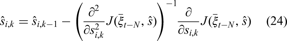

$${\hat{s}}_{i,k}={\hat{s}}_{i,k-1}-{(\frac{{\mathrm{\partial }}^2}{\mathrm{\partial }{s}_{i,k}^2}J({\overline{\xi }}_{t-N},\hat{s}))}^{-1}\frac{\mathrm{\partial }}{\mathrm{\partial }{s}_{i,k}}J({\overline{\xi }}_{t-N},\hat{s})$$

(24)

For large outliers, even with the use of a switching penalty, the switching variable can take very large negative values, resulting in a variable overflow for the intermediate result of $e^{-s_{i,k}}$ . To avoid this issue, it makes sense to place a lower limit on the value of $s_{i,k}$ .

There is one final consideration regarding switching outlier rejection, which is the initial value of the switching variable. For simplicity, we decided to use the Mahalanobis distance based on only the measurement noise (the MHE doesn’t estimate state covariance) of the associated measurement.

Offline evaluation

The presented improvements were evaluated offline, using real UWB measurements gathered in the ”Cyberzoo” test arena at TU Delft. ¹³ We simulated the performance on 12 different flights for TWR and 9 different flights for TDOA. The simulations were performed 10 times with different seeds for the random number generator, for a total of 120 simulations for TWR and 90 simulations for TDOA. For every simulation, all estimators were executed in parallel and saw therefore the same noise. For comparison, we also simulated the initial version of the MHE using the simple gradient (SG) method with a fixed step size and RANSAC for outlier rejection from Pfeiffer et al., ⁸ as well as the EKF from Mueller et al. ³

We compared the different estimators based on three metrics, which are presented in Figure 2 for TWR and in Figure 3 for TDOA.

Success rate: We defined a run to be successful if the root-mean-square error (RMSE) on the position stays below 0.5 m. This definition is somewhat arbitrary but is meant to reflect a value at which the estimator’s accuracy is good enough to allow navigation in spacious indoor environments.

Accuracy: The accuracy of the estimators is assessed using the position RMSE. Unsuccessful runs were removed from the data prior to plotting the accuracy statistics since unsuccessful runs for only a few beacons can easily reach errors of tens of meters and therefore have a tendency to distort the plots.

Normalized computation time: To assess the computational efficiency, we calculated the average computation time per step. For every run, we normalize the average by dividing by the average computation time of the EKF. This was done to reduce the effect of the hardware used and the system load from other sources.

At first glance, we can see, that TWR yields more stable results. The success rate of all estimators is nearly identical and reaches 100% at 5 or 6 beacons. Looking at the accuracy, we can see that all MHE versions outperform the EKF slightly, but no difference can be seen between the different versions.

Figure 1.

Moving Horizon Estimators (MHEs) usually require a lot of computational power. Improvements to our previous work on computationally efficient MHEs allow for on-board execution of the algorithm to localize a nano-copter using Ultra-Wideband measurements.

Figure 2.

Performance of MHE configurations in simulation using TWR measurements: Simple gradient (SG), linesearch (LS) and Newton’s method to solve the minimization problem, random sample consensus (RANSAC) and switching variable outlier rejection (SVOR) for outlier rejection. Shaded regions represent the standard error of the mean.

Figure 3.

Performance of MHE configurations in simulation using TDOA measurements: Simple gradient (SG), linesearch (LS) and Newton’s method to solve the minimization problem, random sample consensus (RANSAC) and switching variable outlier rejection (SVOR) for outlier rejection. Shaded regions represent the standard error of the mean.

The TDOA results are a bit messier. The success rate is quite different between different versions and for many estimators never reaches 100%. It is therefore more interesting to compare the quality of the estimates based on the success rate, rather than based on the accuracy of the successful runs. All MHE variants surpass the EKF in terms of success rate up to 7 beacons. The effect of a constant step size for varying numbers of measurements can be seen in the decreased performance of the simple gradient MHE when the number of beacons increases to 8. Interestingly, using switching variables for outlier rejection (SVOR) seems to be another suitable method for reducing this problem, as seen in the higher success rate. This is likely due to the fact, that SVOR can turn off measurements to keep the magnitude of the gradient closer to constant. This does however mean, that the estimator does not profit from the increased number of measurements, which becomes apparent when looking at the accuracy plots. The most successful approach for dealing with variable gradient magnitudes seems to be the linesearch (LS) approach. We suspect however, that in scenarios that incorporate other measurements (e.g. velocity from optic flow), using Newton’s method will be advantageous.

Let’s finally have a look at the computational efficiency. The EKF clearly still outperforms all versions of the MHE, but as expected, SVOR clearly reduces the computation time compared to RANSAC. Looking at the methods for choosing dynamic step sizes, Newton’s method is more efficient than Linesearch, but still adds some additional cost compared to the simple gradient method.

On-board experiments

To verify our simulation results and demonstrate that the MHE is indeed capable of running on computationally limited devices, we implemented the code on a Crazyflie 2.1. The Crazyflie 2.1. is a small (38 g), versatile platform that can be equipped with a variety of expansion boards, such as the UWB Deck for UWB ranging and the Flow Deck, for altitude and flow measurements. To make full use of the Flow Deck and challenge the versatility of our estimator, we not only used the time-of-flight measurements for altitude, but also incorporated the measurement equations for flow and adjusted the MHE formulation to enable the use of measurements with different units (the flow measurements are in pixels per second). Specifically, we use Newton’s method with SVOR and introduce the inverse covariance matrix of the prior, ${\mathit{P}}^{-1}$ , and the inverse measurement variance, ${\sigma }^2$ as weights in the cost function: ¹⁴

$$\begin{array}{rl}J({\mathit{\xi }}_{t-N},\mathit{s})=& \mu {({\mathit{\xi }}_{t-N}-{\overline{\xi }}_{t-N})}^T{\mathit{P}}^{-1}({\mathit{\xi }}_{t-N}-{\overline{\xi }}_{t-N})\\ & +{\mu }_s\cdot \sum _{k=t-N}^t\sum _{i=1}^m{(s_{i,k}-\overline{s})}^2\\ & +\sum _{k=t-N}^t\sum _{i=1}^m(\mathrm{sig}(s_{i,k})\cdot \frac{\Vert y_{i,k}-{\mathcal{H}}_{i,k}({\mathit{\xi }}_{t-N}){\Vert }^2}{{\sigma }^2})\end{array}$$

(25)

This way, the units of the measurement errors are removed and the measurements are immediately weighted according to their reliability. Each estimator was flown at least five times for a given number of beacons (4, 6 and 8) with the UWB ranging set to TWR. The results in Figure 4 show, that the MHE is indeed able to compete with the EKF in terms of performance for the given scenarios. In terms of computational requirements, we limited the number of measurements the MHE keeps in memory to 80 and used a quality measure based on the switching variable to remove bad measurements before they fall out of the window. With these changes, the MHE runs on-board, using about 25% of the available computational resources, whereas the EKF operates with only about one-fifth of this number. This actually matches quite well with the observations from the offline evaluation.

Figure 4.

Comparison of MHE and EKF using Two-Way Ranging (5 flights per setting).

Conclusion

Moving Horizon Estimation holds a lot of potential, even for computationally limited platforms. By simplifying the problem to an output error MHE and approximating the optimization problem with a single-step gradient descent algorithm, the computational requirements of MHE can be reduced significantly, albeit at the cost of a bit of accuracy. In the end, the MHE slightly outperforms the extended Kalman Filter, which is a popular option for any non-linear state estimation problem.

The use of dynamic step sizes in a single-step gradient descent algorithm helps alleviate problems that occur when the number of incoming measurements varies greatly. Both a linesearch approach and Newton’s method are suitable, but Newton’s method offers more flexibility when dealing with different kinds of measurements.

To further reduce the computational cost, we employed outlier rejection based on switching variables, which offers advantages over RANSAC in terms of computation time.

The improved MHE shows promise in simulation and experiments, where it outperforms a classical EKF and previous iterations of our computationally efficient MHE. The main limitations of the approach are the more complex formulation and the still non-negligible increase in computational cost.

In its current formulation, the MHE only estimates position and velocity, while attitude estimates are provided by the complementary filter. This approach is suitable for pitch and roll, since the gravitational pull can be used as a reference. The yaw estimates on the other hand are subject to drift and currently require proper initialization. This problem should be addressed in future work by including yaw (error) as an additional state in the model.