Trajectory optimization for fully actuated hexacopters: Enhancing maneuverability and applications

Abstract

Several factors need to be taken into account when generating a feasible optimized trajectory. The optimization process heavily relies on the dynamic model of the system. Currently, there are various drone designs available, categorized based on their actuation status. In this study, we apply a trajectory optimization technique to a fully actuated hexacopter (FA-Hex), which is a new application to the best of our knowledge. This type of vehicle has been successfully integrated into several practical applications. Unlike the under-actuated hexacopter (UA-Hex), the FA-Hex can perform maneuvers with minimal banking angles, significantly enhancing the drone’s maneuverability. Our research focuses specifically on trajectory optimization for the FA-Hex and demonstrates the adaptability of our method to different scenarios. We discuss two specific applications: a drone filming without a gimbal joint and a drone with a cable-suspended pendulum. We compare the simulation results with the UA-Hex model to highlight the differences in maneuverability between the two systems. The trajectory optimization is performed offline using CasADi in the MATLAB framework.

Introduction

Aerial robotic systems have found extensive applications in various fields, including package delivery, photography, rescue operations, and construction inspection.^1,2 These missions have led to the development of different types of vehicles tailored to meet specific requirements. Nowadays, aerial systems utilize cable-suspended loads for package delivery in various environments. Additionally, vehicles designed for photography and inspection purposes often integrate a gimbal joint to ensure optimal camera positioning. In these cases, minimizing drone weight and optimizing trajectory and energy consumption are essential objectives. However, striking a balance between control and vehicle design is critical to achieving optimal performance. Aerial vehicle systems can be classified based on their actuation level as under-actuated (UA), fully-actuated (FA), and over-actuated (OV) systems. ³ A quad-rotor drone serves as a common example of an UA system, which relies on total thrust and three torques as virtual control inputs. However, these virtual control inputs are insufficient to directly control all 6 degrees of freedom (DoF) of the system. On the other hand, a FA system possesses a number of virtual controllers equal to the DoF, matching the number of actuators. Conversely, OV drones have an excess number of actuators, enabling them to handle actuator failures using various control allocation techniques. FA vehicles have a more extensive range of maneuvers compared to UA ones. Some drones can adapt to online actuation changes by employing additional servo motors that consider the tilt angle of the motors.

Indeed, hexacopters can be classified as either UA or FA systems based on their actuator configuration. Hexacopters with actuators in one plane, which typically means they have fixed propellers, are considered UA systems. On the other hand, hexacopters equipped with tilting actuators, often known as coaxial hexacopters or hexacopters with tilting propellers, are recognized as FA systems. The ability of the latter to tilt their actuators provides them with greater control authority and maneuverability, allowing them to be fully actuated and perform more complex maneuvers compared to the former.

This work’s primary contribution lies in its flexible approach to solving trajectory optimization problems, which can be adapted to suit a wide range of drone applications. The emphasis lies on scenarios where drones track specific objects through photography. In such cases, it is vital for the drone to maintain a clear field of view of the target by moving with minimal banking angles. Improving the trajectory sent to the low-level controller enhances the drone’s ability to accomplish assigned tasks effectively. Additionally, the FA-Hex can be used for package delivery with the help of a cable-suspended pendulum mechanism. This setup enables the drone to reduce oscillations and perform precise maneuvers, even in challenging and static environments.

Design and control strategies

Various vehicle design and control strategies have been developed and utilized to manage the dynamics of FA drones. Employing these vehicles offers the key advantage of independent attitude and altitude control by decoupling their dynamics. ⁴ Non-linear control based on full geometric control, ensuring precise position tracking, is applied by Franchi et al. ⁵ and Ryll et al. ⁶ Stability of the resulting controller is established using Lyapunov techniques. Furthermore, Rajappa et al. ⁷ proposes an optimal design for the tilted angle based on the active set of possible wrenches exerted by the FA drone, using a feedback linearization control approach with a PID controller to decouple position and orientation control. Another approach is presented in Odelga et al., ⁸ by adding a tilting mechanism to the motors of the UA drone, incorporating two servo actuators to rotate the rotor’s angle in radial and tangential directions around the arm. Feedback-linearization control is employed for managing the drone’s dynamics. To handle environmental perturbations, Arizaga et al., ⁹ uses adaptive control for the FA-Hex drone. Similarly, Arizaga et al. ¹⁰ proposes adaptive sliding mode control for FA-Hex drones with a cable-suspended pendulum, compensating for the inability to measure the load’s position by developing an extended gain observer-based adaptive sliding mode approach.

Trajectory optimization

Generating a reference trajectory to be tracked by the lower-level controllers is a demanding task when working with FA vehicles. Currently, the literature review on trajectory optimization primarily focuses on UA vehicles. Therefore, it becomes a challenging problem to develop an optimal controller that generates desired positions and orientations for FA vehicles. The research in this area can be categorized into two main approaches. Firstly, a differential flatness approach is utilized to obtain a smooth and feasible trajectory.^11–14 Secondly, the dynamical model is incorporated as a constraint in the optimization problem.^15–17 Utilizing the differential flatness approach in formulating the optimization problem has shown to reduce computational time. It has been demonstrated by Sreenath and Lee ¹⁴ that the UA quad-rotor drones are differential flat systems, which can be characterized by the following flat output vector: position $(x,y,z)$ and heading $(\psi )$ , of the system. In contrast, FA vehicles are considered to be differential flat based on the full dynamics of the drone. In our approach, we have chosen to incorporate the dynamical system as a constraint in the optimization problem. Differential flatness is utilized to generate the trajectory of an UA vehicle, which is then used as an initial condition for the optimization problem of the FA-Hex vehicle. This overview is the basis of our contribution to the study of a trajectory optimization problem for FA vehicles, taking into account specific objectives.

We organize the remainder of the paper as follows. In Sections and, we present the mathematical model of the FA-Hex and the extended model that incorporates a cable-suspended pendulum, and in Section “Trajectory optimization problem”, we formulate the proposed trajectory optimization problem. In Section “Simulations” the simulation results are presented based on the defined optimization problem.

Model and system variables

The importance of the dynamical system in achieving workable results, as mentioned earlier, makes it necessary to define the mathematical model of the system we’re looking at. In this section, we present the dynamic model of the FA-Hex and its extension to include the cable-suspended pendulum. The model is derived from Newton’s Euler equation, while taking into account the following assumptions:

The drone is assumed to be a rigid body.

The drone is assumed to be symmetric with respect to its axis, and its inertia matrix is diagonal and denoted as $I_B=\left[\begin{array}{ccc}{I}_{xx}& 0& 0\\ 0& I_{yy}& 0\\ 0& 0& I_{zz}\end{array}\right]$ .

FA-Hex modeling

The modeling approach of the drone involves two main frames: the inertial frame $({\mathcal{F}}_I)$ defined by $(x_I,y_I,z_I)$ axis, and the body frame $({\mathcal{F}}_{\mathcal{B}})$ defined by $(x_B,y_B,z_B)$ axis, as illustrated in Figure 1. The rotation between ${\mathcal{F}}_{\mathcal{I}}$ and ${\mathcal{F}}_{\mathcal{B}}$ is defined by the Euler angles $\mu =[\varphi ,\theta ,\psi {]}^T$ and the corresponding rotational matrix $R(\mu )$ where:

$$R(\mu )=\left[\begin{array}{ccc}{C}_{\psi }{C}_{\theta }& C_{\psi }{S}_{\theta }{S}_{\varphi }-S_{\psi }{C}_{\varphi }& C_{\psi }{S}_{\theta }{C}_{\varphi }+S_{\psi }{S}_{\theta }\\ S_{\psi }{C}_{\theta }& S_{\psi }{S}_{\theta }{S}_{\varphi }+C_{\psi }{C}_{\varphi }& S_{\psi }{S}_{\theta }{C}_{\varphi }-C_{\psi }{S}_{\varphi }\\ -S_{\theta }& C_{\theta }{S}_{\varphi }& C_{\theta }{C}_{\varphi }\end{array}\right]$$

with the notations $C_{*}=cos(*)$ and $S_{*}=sin(*).$

Figure 1.

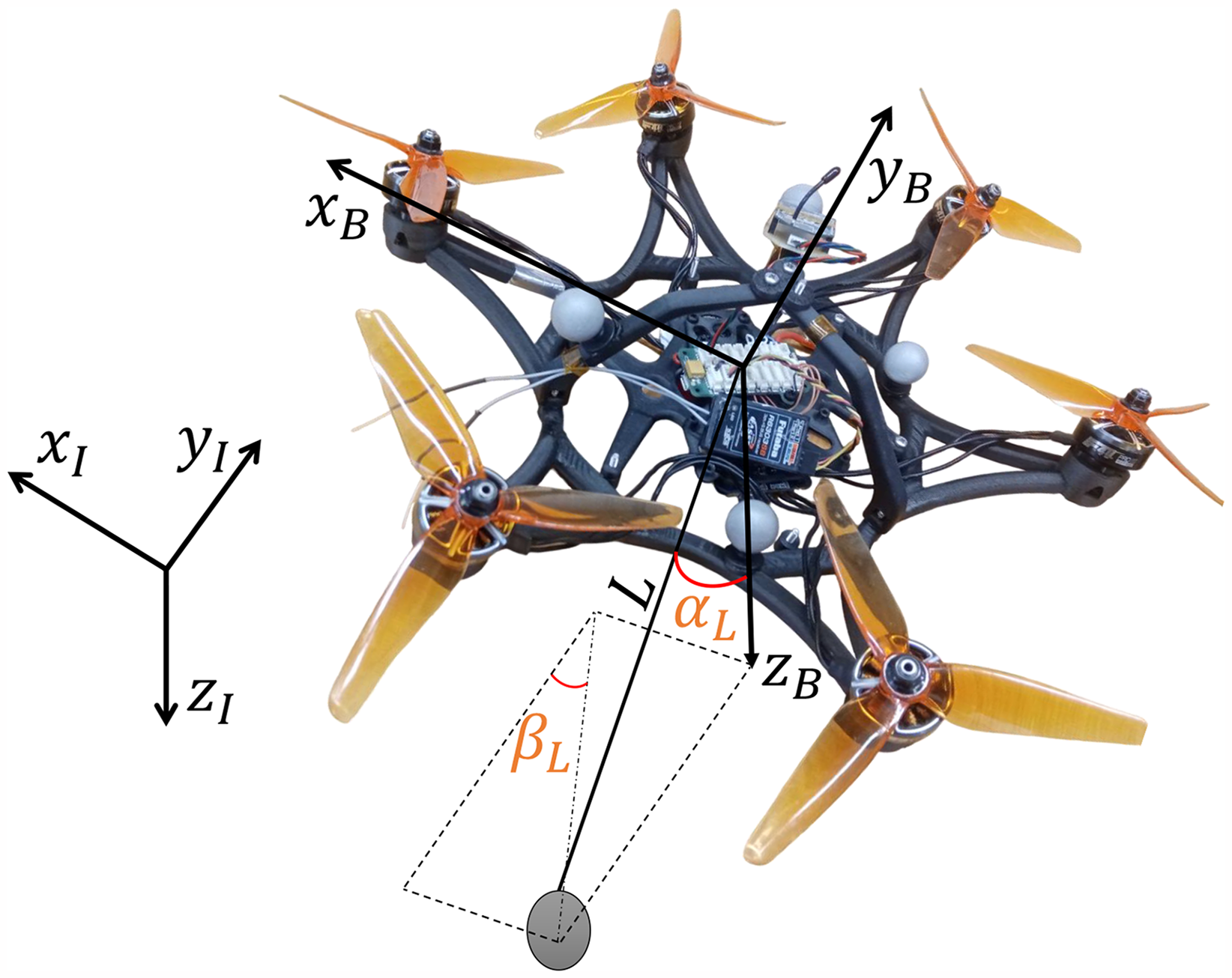
Fully Actuated Hexacopter attached to a payload with Inertial ( ${\mathcal{F}}_{\mathcal{I}}$ ) and Body ( ${\mathcal{F}}_{\mathcal{B}}$ ) Frames. The cable suspended pendulum is described by two angles ${\alpha }_L$ and ${\beta }_L$ along the z-axes and the inertial lateral plane $(x_I{y}_I)$ respectively.

The position of the drone in the inertial frame is denoted as $\xi =[x,y,z{]}^T$ , and its translation velocity is represented by $v=[v_x,v_y,v_z{]}^T$ . The angular velocity in the body frame is given by $\mathrm{\Omega }=[p,q,r{]}^T$ . The relationship between the Euler rates $\dot{\mu }$ and the angular body rates $\mathrm{\Omega }$ is expressed by the transformation matrix $W(\mu )$ , where $\dot{\mu }=W(\mu {)}^{-1}\mathrm{\Omega }$ such that

$$\left[\begin{array}{c}\dot{\varphi }\\ \dot{\theta }\\ \dot{\psi }\end{array}\right]=\left[\begin{array}{ccc}1& S_{\varphi }{T}_{\theta }& C_{\varphi }{T}_{\theta }\\ 0& C_{\varphi }& -S_{\varphi }\\ 0& S_{\varphi }/C_{\theta }& C_{\varphi }/C_{\theta }\end{array}\right]\left[\begin{array}{c}p\\ q\\ r\end{array}\right]$$

where $T_{*}=tan(*)$ . The states of the FA-Hex are defined as $x=[{\xi }^T,v^T,{\mu }^T,{\mathrm{\Omega }}^T{]}^T$ , and the system dynamics are expressed as follows:

$$\dot{\xi }=v$$

(1)

$$m\ddot{\xi }=mg+R(\mu )\sum _{i=1}^6{F}_{B_i}$$

(2)

$$I_B\dot{\mathrm{\Omega }}=\sum _{i=1}^6{\tau }_{B_i}-\mathrm{\Omega }\times I_B\mathrm{\Omega }$$

(3)

Here, $\times$ is the cross product operator, whereas $F_{B_i}=[F_{x_i}{F}_{y_i}{F}_{z_i}{]}^T$ and ${\tau }_{B_i}=[{\tau }_{x_i}{\tau }_{y_i}{\tau }_{z_i}{]}^T$ represent the forces and torques exerted by the $i$ -th motor expressed in the body frame, respectively. $F_{B_i}$ and ${\tau }_{B_i}$ depend on the propeller’s angular speed ${\omega }_i$ , as well as the motor’s orientation ${\alpha }_i$ within the drone’s geometric frame, and the tangential orientation $\beta$ defined as the angle between the motor’s axis $z_{m_i}$ and the drone’s $z_B$ axis. This is represented in Figure 2, where $F_i=\sqrt{F_{x_i}^2+F_{y_i}^2}$ is the projection of $F_{B_i}$ in the $(x_B\text{,}{y}_B)$ plane. The expressions of $F_{B_i}$ and ${\tau }_{B_i}$ are given in Table 1. It can be checked that $F_{B_i}=F_{thrus{t}_i}$ , where $\Vert F_{thrus{t}_i}\Vert =k_t{\omega }_i^2$ , while ${\tau }_{B_i}={\tau }_{thrus{t}_i}+{\tau }_{dra{g}_i}$ , where $\Vert {\tau }_{thrus{t}_i}\Vert =k_{t}l{\omega }_i^2$ and $\Vert {\tau }_{dra{g}_i}\Vert =k_q{\omega }_i^2$ . $k_t$ , $k_q$ and $l$ stand for the thrust coefficient, the drag coefficient, and the distance between the $i$ -th motor and the drone’s center of mass respectively.

Figure 2.

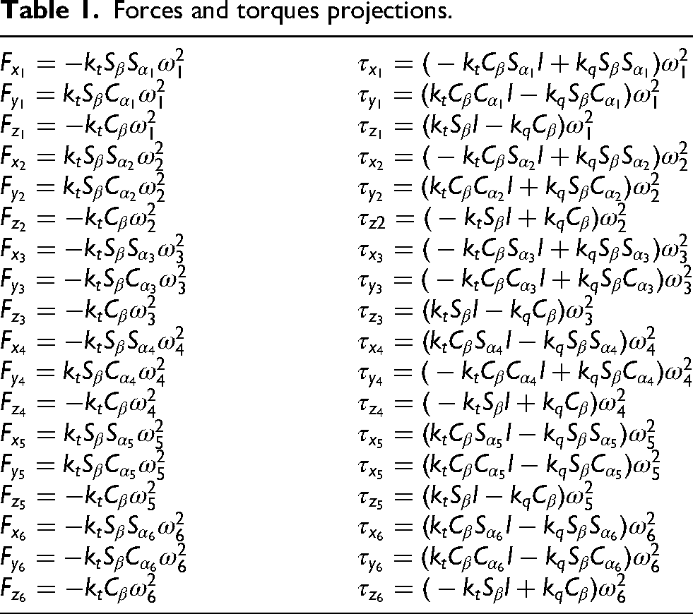
Forces projection in the lateral plane with the motor tilting angles $\beta$ between $z_B$ and $z_{m_i}$ the axis of the $i$ -th motor.

Table 1.

Forces and torques projections.

$F_{x_1}=-k_t{S}_{\beta }{S}_{{\alpha }_1}{\omega }_1^2$	${\tau }_{x_1}=(-k_t{C}_{\beta }{S}_{{\alpha }_1}l+k_q{S}_{\beta }{S}_{{\alpha }_1}){\omega }_1^2$
$F_{y_1}=k_t{S}_{\beta }{C}_{{\alpha }_1}{\omega }_1^2$	${\tau }_{y_1}=(k_t{C}_{\beta }{C}_{{\alpha }_1}l-k_q{S}_{\beta }{C}_{{\alpha }_1}){\omega }_1^2$
$F_{z_1}=-k_t{C}_{\beta }{\omega }_1^2$	${\tau }_{z_1}=(k_t{S}_{\beta }l-k_q{C}_{\beta }){\omega }_1^2$
$F_{x_2}=k_t{S}_{\beta }{S}_{{\alpha }_2}{\omega }_2^2$	${\tau }_{x_2}=(-k_t{C}_{\beta }{S}_{{\alpha }_2}l+k_q{S}_{\beta }{S}_{{\alpha }_2}){\omega }_2^2$
$F_{y_2}=k_t{S}_{\beta }{C}_{{\alpha }_2}{\omega }_2^2$	${\tau }_{y_2}=(k_t{C}_{\beta }{C}_{{\alpha }_2}l+k_q{S}_{\beta }{C}_{{\alpha }_2}){\omega }_2^2$
$F_{z_2}=-k_t{C}_{\beta }{\omega }_2^2$	${\tau }_{z2}=(-k_t{S}_{\beta }l+k_q{C}_{\beta }){\omega }_2^2$
$F_{x_3}=-k_t{S}_{\beta }{S}_{{\alpha }_3}{\omega }_3^2$	${\tau }_{x_3}=(-k_t{C}_{\beta }{S}_{{\alpha }_3}l+k_q{S}_{\beta }{S}_{{\alpha }_3}){\omega }_3^2$
$F_{y_3}=-k_t{S}_{\beta }{C}_{{\alpha }_3}{\omega }_3^2$	${\tau }_{y_3}=(-k_t{C}_{\beta }{C}_{{\alpha }_3}l+k_q{S}_{\beta }{C}_{{\alpha }_3}){\omega }_3^2$
$F_{z_3}=-k_t{C}_{\beta }{\omega }_3^2$	${\tau }_{z_3}=(k_t{S}_{\beta }l-k_q{C}_{\beta }){\omega }_3^2$
$F_{x_4}=-k_t{S}_{\beta }{S}_{{\alpha }_4}{\omega }_4^2$	${\tau }_{x_4}=(k_t{C}_{\beta }{S}_{{\alpha }_4}l-k_q{S}_{\beta }{S}_{{\alpha }_4}){\omega }_4^2$
$F_{y_4}=k_t{S}_{\beta }{C}_{{\alpha }_4}{\omega }_4^2$	${\tau }_{y_4}=(-k_t{C}_{\beta }{C}_{{\alpha }_4}l+k_q{S}_{\beta }{C}_{{\alpha }_4}){\omega }_4^2$
$F_{z_4}=-k_t{C}_{\beta }{\omega }_4^2$	${\tau }_{z_4}=(-k_t{S}_{\beta }l+k_q{C}_{\beta }){\omega }_4^2$
$F_{x_5}=k_t{S}_{\beta }{S}_{{\alpha }_5}{\omega }_5^2$	${\tau }_{x_5}=(k_t{C}_{\beta }{S}_{{\alpha }_5}l-k_q{S}_{\beta }{S}_{{\alpha }_5}){\omega }_5^2$
$F_{y_5}=k_t{S}_{\beta }{C}_{{\alpha }_5}{\omega }_5^2$	${\tau }_{x_5}=(k_t{C}_{\beta }{C}_{{\alpha }_5}l-k_q{S}_{\beta }{C}_{{\alpha }_5}){\omega }_5^2$
$F_{z_5}=-k_t{C}_{\beta }{\omega }_5^2$	${\tau }_{z_5}=(k_t{S}_{\beta }l-k_q{C}_{\beta }){\omega }_5^2$
$F_{x_6}=-k_t{S}_{\beta }{S}_{{\alpha }_6}{\omega }_6^2$	${\tau }_{x_6}=(k_t{C}_{\beta }{S}_{{\alpha }_6}l-k_q{S}_{\beta }{S}_{{\alpha }_6}){\omega }_6^2$
$F_{y_6}=-k_t{S}_{\beta }{C}_{{\alpha }_6}{\omega }_6^2$	${\tau }_{y_6}=(k_t{C}_{\beta }{C}_{{\alpha }_6}l-k_q{S}_{\beta }{C}_{{\alpha }_6}){\omega }_6^2$
$F_{z_6}=-k_t{C}_{\beta }{\omega }_6^2$	${\tau }_{z_6}=(-k_t{S}_{\beta }l+k_q{C}_{\beta }){\omega }_6^2$

FA-Hex modeling with cable suspended pendulum

The FA-Hex system with the cable-suspended payload operates in a hybrid mode, which relies on the tension force in the cable, as discussed in Sreenath and Lee. ¹⁴ The payload’s behavior is modeled under two main scenarios: taut and slack cables. The transition between these modes adds intricacy to the modeling approach, thus augmenting the complexity of the optimization function. Nevertheless, by introducing a linear complementary constraint into the optimization problem, it is feasible to eliminate the necessity for the hybrid model. ¹⁵

The state vector of the model is expanded and modified to incorporate both the position and velocity of the load. This state is denoted as $x=[{\xi }^T,v^T,{\mu }^T,{\mathrm{\Omega }}^T,{\xi }_L^T,v_L^T{]}^T$ , where ${\xi }_L=[x_L,y_L,z_L{]}^T$ represents the load’s position in the inertial frame, and $v_L=[v_{L_x},v_{L_y},v_{L_z}{]}^T$ represents the load’s velocity. With the presence of the load, a new tension force $T$ comes into play, affecting the drone’s dynamics. Furthermore, due to the cable’s rotation around the inertial axis, a unit vector describing a rotation $R_L(\eta )$ is introduced to take account of the drone’s orientation in relation to the load. Here, $\eta =[{\alpha }_L,{\beta }_L{]}^T$ , as depicted in Figure 1.

$$R_L(\eta )=\left[\begin{array}{c}\sin ({\alpha }_L)\cos ({\beta }_L)\\ \sin ({\alpha }_L)\sin ({\beta }_L)\\ \cos ({\alpha }_L)\end{array}\right]$$

The extended dynamic model is then represented as follows:

$$\dot{\xi }=v$$

(4)

$$(m+m_L)\ddot{\xi }=(m+m_L)g+R(\mu )\sum _{i=1}^6{F}_{B_i}+T{R}_L(\eta )$$

(5)

$$I_B\dot{\mathrm{\Omega }}=\sum _{i=1}^6{\tau }_{B_i}-\mathrm{\Omega }\times I_B\mathrm{\Omega }$$

(6)

$${\xi }_L=\xi +R_L(\eta )L$$

(7)

$${\dot{\xi }}_L=v_L$$

(8)

$${\ddot{\xi }}_L=m_{L}g-T{R}_L(\eta )$$

(9)

where $T$ is the tension in the cable, $L$ is the length of the cable, and $m_L$ is the mass of the load respectively.

Trajectory optimization problem

Optimization methods are employed to address trajectory optimization problems by minimizing a cost function, while taking into account different constraints. To achieve a viable and physically relevant solution, the optimization problem needs to encompass the system dynamics along with the practical restrictions on the states and inputs. Broadly, optimization problems fall into two primary categories: direct methods ¹⁸ and indirect methods. ¹⁶

The indirect method involves formulating the optimization problem as a boundary value problem (BVP) and solving it by defining the co-state vector. It is worth mentioning that the model of the system is incorporated into the Hamiltonian-Jacobian-Bellman equation, which is solved using the BVP approach. On the other hand, the direct optimization problem takes into account a discrete dynamical model along with its constraints. The main distinction between the two methods lies in the integration aspect. Direct methods are known for incorporating integrated solutions for the dynamical model within their approach. It is worth noting that indirect methods generally tend to be more accurate than direct methods, provided that a good initial guess can be obtained, which can be challenging in practice. However, in the realm of robotics applications, direct methods are widely utilized for designing optimal controllers. This preference is largely attributed to their expansive region of convergence. ¹⁹

In this work, our focus is on utilizing a direct method to obtain the optimal trajectory. Direct methods can be formulated using shooting and collocation methods, with the choice depending on the specific dynamical equation. When an explicit model is available, the shooting method is often employed. This method involves decomposing the trajectory into sub-optimal intervals and calculating the spline between each interval. The formulation can be done through single shooting, where only the state variables are optimized, or multiple shooting, where both control inputs and states are optimized at each control interval. The resulting discrete problem is then addressed using non-linear programming methods. ¹⁸

General problem formulation

We pose our trajectory optimization problem as follows :

$$\begin{array}{cc}\underset{x,u}{min}& J(x,u)\\ \mathrm{s}.\mathrm{t}.& g(x,u)=0& f(x,u)\ge 0\end{array}$$

(10)

In this formulation, $x$ represents the state vector of the system, and $u$ denotes the angular speed of each motor. The equality constraints $g(x,u)$ encompass various constraints, including the dynamical constraint of the system, while the inequality constraints $f(x,u)$ define additional inequality restrictions. To solve the optimization problem, we divide the trajectory into N control sub-intervals. For this purpose, we employ the direct multiple shooting optimization formulation, which offers several advantages over other techniques. ¹⁸

FA-Hex

First, we will define the optimization problem for the FA-Hex targeting photography application.

Cost Function: The cost function to be minimized is defined as follows:

$$\underset{x}{min}J=S_f{t}_f+{\int }_0^{t_f}{x}^{T}Qxdt$$

(11)

Here, $x=[{\xi }^T,v^T,{\mu }^T,{\mathrm{\Omega }}^T{]}^T$ and $Q\in {\mathcal{R}}^{12\times 12}$ represents the weight cost assigned to the states of the system, $t_f$ is the time allotted to the whole scenario, and $S_f$ denotes the slack weight used to handle the priority of the specified time.

Dynamical Model Constraint: The dynamical model, defined in Section “FA-Hex modeling”, is discretized using fourth-order Runge-Kutta. This model is employed to ensure the attainment of dynamically feasible states by solving $x_{k+1}=h(x_k,u_k)$ , where $h$ is a vector field representing the discretized dynamical model of the system.

Multiple-Shooting Constraint: The method involves computing the next state using the discretized model. The computed next state is constrained to align with the optimized parameter, which can be achieved by ensuring that $x_{\text{next}}-x_k=0$ . Here, $x_k$ represents the system state at the $k$ -th interval, and $x_{\text{next}}$ corresponds to the state calculated using the discretized dynamical model.

Boundary Conditions: To ensure that the optimization problem begins and ends within feasible constraints, additional boundary constraints are included. The variables $x_{\text{initial}}$ and $x_{\text{,final}}$ are defined and incorporated into the equality constraint $g(x,u)$ as $x_0-x_{\text{initial}}=0$ and $x_N-x_{\text{,final}}=0.$

State and Input Constraint: The states and inputs of the system should not exceed their respective boundaries. To enforce this requirement, two additional equations (12, 13) are introduced to the function $f(x,u)$ .

$$x_{min}\le x_k\le x_{max}$$

(12)

$$u_{min}\le u_k\le u_{max}$$

(13)

Waypoint Navigation Constraint: The primary objective of this work is to navigate and fly over specific points. To achieve this goal, an additional constraint is introduced: $w_p-\delta <x_k<w_p+\delta$ , where $w_p$ represents the specified waypoint. The inclusion of $\delta$ in this equation ensures the robustness of the algorithm and helps avoid excessive equality constraints. It is important to note that this problem does not aim to optimize time since such optimization conflicts with the defined constraint. For more detailed information on time-optimal trajectory optimization the reader can refer to Foehn et al. ²⁰

FA-Hex with cable suspended pendulum

In this section, we will introduce the extended constraints and objective function that are used to optimize the trajectory for FA-Hex with a cable-suspended pendulum.

Cost Function: The extended cost function to be minimized on the variables is defined as follows:

$$\begin{array}{c}\underset{x,T,L}{min}J=S_f{t}_f+{\displaystyle {\int }_0^{t_f}{x}_{ext}^T{Q}_L{x}_{ext}dt}\\ +{\displaystyle {\int }_0^{t_f}({\overline{R}}_{0}T+{\overline{R}}_1(L_0-L))dt}\end{array}$$

(14)

Here, $x_{ext}=[{\xi }^T,v^T,{\mu }^T,{\mathrm{\Omega }}^T,{\xi }_L^T,v_L^T{]}^T$ , $Q_L\in {\mathcal{R}}^{18\times 18}$ and the added terms ${\overline{R}}_{0}T$ and ${\overline{R}}_1(L_0-L)$ represent the cost associated with the taut and slack modes of the cable, where ${\overline{R}}_0$ and ${\overline{R}}_1$ are scalar weights, and $L_0$ is the initial length of the load in taut mode. These terms are included in the objective function to address the hybrid modeling problem of the pendulum. The trajectory is generated with a corresponding slack and taut mode, based on the weighting values.

Dynamical Model Constraint: The extended dynamical model introduced in Section ‘FA-Hex modeling with cable suspended pendulum” is also discretized using fourth-order Runge-Kutta and incorporated into the equality constraints $g(x,u)$ .

Linear Complementary Constraint: This constraint is added to eliminate the hybrid dynamical model, assuming that either the slack mode or the taut mode is present. It is represented by $T(L_0-L)$ , where $L_0$ is the cable length when taut, and $T$ represents the tension in the cable.

Tension Boundaries Constraint: To ensure a realistic and feasible solution, it is important to impose bounds on the tension. This can be achieved by incorporating the constraint $0\le T\le T_{\text{max}}$ , where $T_{\text{max}}$ represents the maximum allowable tension. The value of $T_{\text{max}}$ can be determined based on prior information or known limitations of the system.

Cable Length Constraint: In addition to the complementary constraint, the length of the cable should be positive, $L\ge 0$ .

Payload Swung Angle Constraint: To prevent swinging and potential collisions with the drone, a constraint is introduced as ${\alpha }_L\ge {\alpha }_{L_{\text{min}}}\text{and}{\alpha }_L\le {\alpha }_{L_{\text{max}}}$ .

The other constraints defined in the FA-Hex drone are primarily utilized as constraints for this particular application.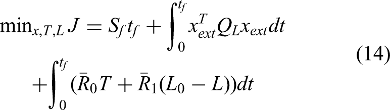

Simulations

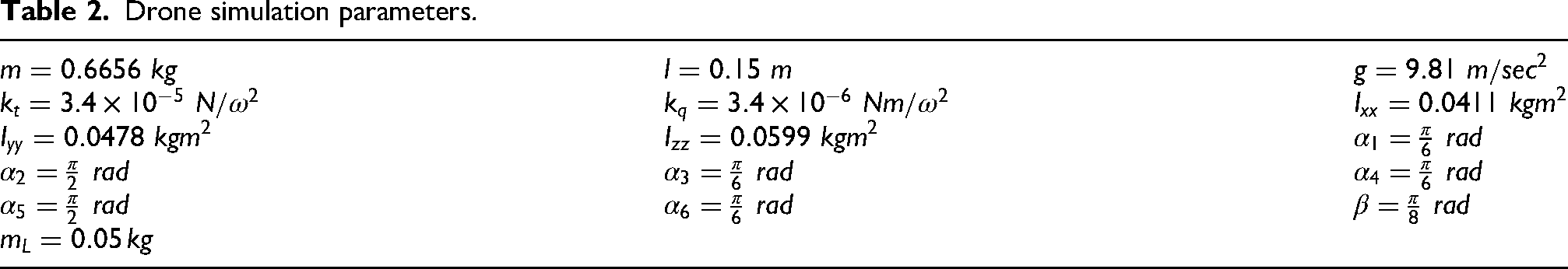
The defined optimization problem is formulated as a nonlinear optimization problem using the CasADi Toolbox. ²¹ As mentioned earlier, this study considers two primary scenarios: simple FA-Hex and FA-Hex with a cable-suspended pendulum. A comparison between FA-Hex and UA-Hex is accomplished showing the enhancing of maneuverability of the FA-Hex. The drone parameters used to simulate the drone model are presented in Table 2.

Table 2.

Drone simulation parameters.

$m=0.6656kg$	$l=0.15m$	$g=9.81{m/sec}^2$
$k_t=3.4\times {10}^{-5}N/{\omega }^2$	$k_q=3.4\times {10}^{-6}Nm/{\omega }^2$	$I_{xx}=0.0411{kgm}^2$
$I_{yy}=0.0478{kgm}^2$	$I_{zz}=0.0599{kgm}^2$	${\alpha }_1=\frac{\pi }{6}rad$
${\alpha }_2=\frac{\pi }{2}rad$	${\alpha }_3=\frac{\pi }{6}rad$	${\alpha }_4=\frac{\pi }{6}rad$
${\alpha }_5=\frac{\pi }{2}rad$	${\alpha }_6=\frac{\pi }{6}rad$	$\beta =\frac{\pi }{8}rad$
$m_L=0.05kg$

FA-Hex and UA-Hex trajectory generation

The scenario involves the drone passing through multiple waypoints. To assess the algorithm’s ability to achieve minimal banking angles, several test cases were conducted. A trajectory comprising four points is shown in Figure 3. The time allotted for this scenario is $t_f=8s$ , with $N=100$ control intervals. It’s worth noting that, as classified by Franchi et al., ⁵ FA vehicles belong to the category of Lateral Bounded Force vehicles (LBF). In these vehicles, lateral acceleration is constrained to be smaller than the vertical acceleration of the drone. The UA-Hex shares the same parameters as the FA-Hex, except for having a tilting rotor angle $\beta =0$ . The achieved velocity of the FA-Hex is approximately $1.5m/s$ when flying without banking, while the velocity of the UA-Hex can reach $2.5m/s$ . Figure 4 displays the optimized Euler angles for both the UA-Hex and FA-Hex in the considered scenario. Clearly, based on the optimized trajectory, the FA-Hex maintains banking angles close to zero degrees while striving to achieve the same trajectory.

Figure 3.

Projection in the horizontal plane of the optimized trajectory for FA-Hex and UA-Hex drones as they fly between specified points and then return to their intial positions. The points are defined by their coordinates: $P1=[0,-1,1.3]$ , $P2=[2,-1,1.3]$ , $P3=[2,1.5,1.8]$ and $P4=[0,1.5,1.8]$ .

Figure 4.

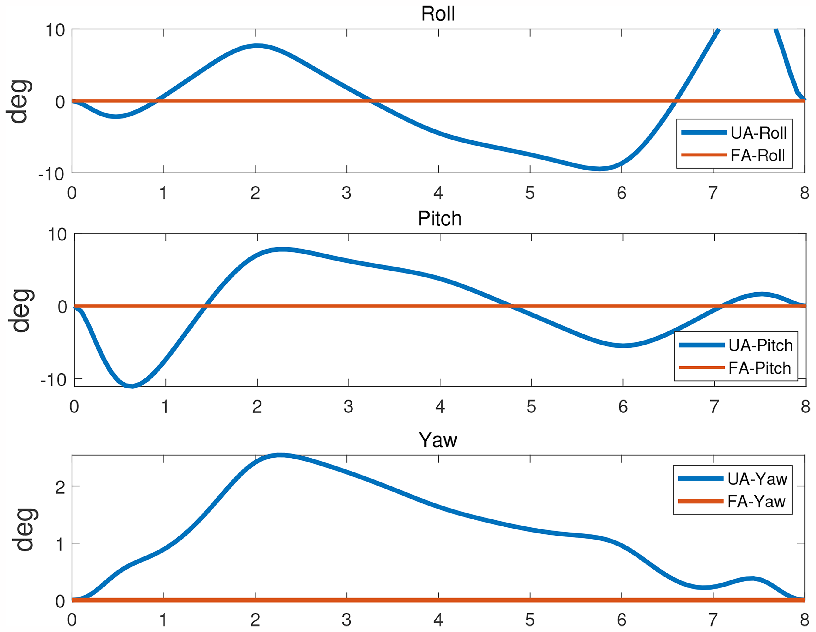
Euler angles comparison between FA-Hex and UA-Hex.

FA-Hex with cable suspended pendulum

In another application, the optimization problem is expanded, as explained in Section “FA-Hex with cable suspended pendulum”, to be solved across the optimization variables $x,u,T,L,$ and $q$ . As in Section “FA-Hex and UA-Hex trajectory generation”, the scenario involves flying between predetermined points. Utilizing linear complementary constraints, it becomes feasible to generate a trajectory with minimal slack, indicating that the cable length remains close to $L_0$ for the majority of the trajectory. The simulation results are depicted in Figure 5, illustrating both the payload and drone trajectories.

Figure 5.

Projection in the horizontal plane of the optimized trajectory for FA-Hex with cable suspended pendulum.

Initial guess

The initial guess plays a pivotal role in ensuring the optimization problem converges to its optimal solution. Providing a feasible initial guess that closely approximates the expected solution is essential. This step is critical for achieving convergence and reducing computational time needed to solve the problem. In this context, it is important to note that the drone is initially treated as a UA system. The differential flatness approach is employed to generate an initial guess for the problem. Furthermore, motion planning algorithms grounded in graph theory, such as the $A*$ and $RTT$ algorithms, can be employed. These algorithms facilitate the creation of a global path, effectively aiding in solving the trajectory planning problem.

Conclusion and extensions

In this work, we have proposed a trajectory optimization formulation for FA-Hex systems. The simulations demonstrate the feasibility of this approach by generating trajectories with minimal banking angles. However, the algorithms used in this study have certain constraints when it comes to defining the nodes and time. The algorithm shows fast performance when when the trajectory is divided into $N=100$ control intervals, taking only a few seconds to converge to the optimal solution. Future work could involve extending the problem to incorporate avoidance of static defined obstacles by implementing specific maneuvers. As an extension of this paper, we are currently working on the identification and control of the real FA-Hex system. Our objective is to conduct real experimental flights to test the optimized trajectory in the mentioned scenarios. The planned tests will utilize the Paparazzi autopilot ²² with a modified INDI controller or feedback linearization.