Sage Journals: Discover world-class research

Abstract

Unmanned Aircraft Systems (UAS) has become widespread over the last decade in various commercial or personal applications such as entertainment, transportation, search and rescue. However, this emerging growth has led to new challenges mainly associated with unintentional incidents or accidents that can cause serious damage to civilians or disrupt manned aerial activities. Machine failure makes up almost 50% of the cause of accidents, with almost 40% of the failures caused in the propulsion systems. To prevent accidents related to mechanical failure, it is important to accurately estimate the Remaining Useful Life (RUL) of a UAS. This paper proposes a new method to estimate RUL using vibration data collected from a multi-rotor UAS. A novel feature called mean peak frequency, which is the average of peak frequencies obtained at each time instance, is proposed to assess degradation. The Long Short-Term Memory (LSTM) is employed to forecast the subsequent 5 mean peak frequency values using the last 7 computed values as input. If one of the estimated values exceeds the predefined 50 Hz threshold, the time from the estimation until the threshold is exceeded is calculated as the RUL. The estimated mean peak frequency values are compared with the actual values to analyze the success of the estimation. For the 1st, 2nd, and 3rd replications, RUL results are 4 s, 10 s, and 10 s, and root mean square error (RMSE) values are 3.7142 Hz, 1.4831 Hz, and 1.3455 Hz, respectively.

Keywords

Unmanned Aircraft Systems machine learning predictive maintenance vibration signals remaining useful life

Introduction

Although unmanned aircraft systems (UAS) have been used in military operations for a long time, they have recently become more appealing in civil aviation such as commercial and healthcare applications that are subjected to fly across urban areas to deliver packages or medical products.^1–3

With the increase in civilian use of UAS, there has been a significant increase in UAS accident rates, with a recorded accident rate of 100 times more than manned aircraft.^4–6 It was found that 33 to 67% of accidents involving UAS were caused by failures associated with mechanical or electrical components.^7,8 In addition, it was determined that 23 to 53% of the system failures occurred in the propulsion system of the UAS, where the main components are the rotor and propeller.^9,10 Even though many developments within the design of UAS have taken place over the years, potential errors still occur in the propulsion system.^11,12 Hence, it is crucial to prevent machine failures in the propeller systems of UAS.

In 2019, the EU published very tight regulations to enforce safe, sustainable, and secure UAS operations.^13–15 Consequently, new UAS must be individually reliable and equipped with systems to mitigate or avoid both aerial and ground risks, such as collisions with other flying objects or collisions with humans and critical infrastructures. Since a major malfunction that may occur during the flight may increase the ground risks, the current and anticipated health state of the UAS should be constantly monitored, and at the same time, the possible landing spots are visually identified and stored.

The current work aims to develop data-driven predictive maintenance (PdM) model that can predict remaining useful life (RUL). Thus, it can predict a malfunction that may occur and a landing decision can be made accordingly. The model employs vibration data collected from a multi-rotor UAS, signal processing, and machine learning methods. To the best of the authors’ knowledge, this is the first benchmark research study that employs the time-frequency domain feature in the RUL prediction of UAS. Accordingly, in this study, the short-time Fourier Transform was applied to pre-processed vibration data to obtain the spectrogram. After obtaining the spectrograms for each time interval, peak frequencies were found and averaged. This article contributes to knowledge by also providing an open-source vibration data that can be utilized for RUL estimation in UAS.

The paper is organized as follows: Section ‘Literature review’ reviews existing solutions and the related work in the area of predictive maintenance. In Section ‘Methodology for RUL estimation’, the materials and methods used in the study are explained in detail. Section ‘Testing and results’ illustrates the results of the proposed methodology. Finally, it is followed by a conclusion in Section ‘Conclusions’.

Literature review

The idea of Industry 4.0 has greatly encouraged the use of digital technologies in the manufacturing industry to manufacture faster, cheaper and less error-prone.^16–18 With the use of digital technologies in the manufacturing industry, production errors caused by malfunctions that may occur in machines and even planned and unplanned downtimes that increase production costs excessively are reduced with appropriate maintenance strategies.^19–21 The PdM is a maintenance strategy that utilizes collected data from sensors, monitoring machine/equipment status, and processing data by statistical/ machine learning methods to estimate the future condition of machine/equipment, the time of failure or the RUL that is the time until the machine can no longer perform its desired function and maintenance or replacement is needed.^22–24 In this regard, there are three main approaches to estimating the RUL of a machine: the survival model,^25,26 which is used when only data from the time of failure is available, the degradation model,^27,28 which is used when failure data is not available but a safety threshold that signals failure is known, and the similarity model,^29,30 which is used when the entire history of a similar machine, from good health to failure, is known.

The PdM can be defined into four main categories knowledge-based, physics-based, data-driven and digital twin methods,^31–33 each of which has some pros and cons. The knowledge-based method relies on experience identifying the fault by evaluating the similarity between a monitored case and a library of previously known faults. The drawbacks are the difficulty in obtaining accurate information from experience and limited access to knowledgeable experts.^34,35 Similarly, the physics-based method is based on the laws of physics and mathematics to evaluate the degradation behavior with sparse data collection. However, it is very difficult to create such a model as most machines consist of complex mechanical and electrical systems that are difficult to formulate mathematically.^35,36 In data-driven methods, the data obtained from the sensors is processed by machine learning methods and used to examine the deterioration of components or the current health status of the system or its RUL. However, these models use computational power and a large amount of data.^37,38 Digital Twin integrates physics-based with real-time data to have a virtual representation of the physical system or process.³⁹ Among these approaches, the data-driven model has emerged as a powerful tool for predictive maintenance applications since these models are capable of dealing with and capturing complex relationships among data, which is difficult to obtain using physics-based or knowledge-based models as well as the degradation behaviour, the health status and its RUL can be mined by data processing and machine learning methods.

Due to the development of sensor technology in recent years, data obtained from temperature, pressure, lubricant, noise and vibration sensors are used in predictive maintenance activities. The decision about which sensor data to use depends on both the type of problem to be investigated and the operating conditions of the machine. Vibration analysis has been the most widely used PdM technique in rotating or reciprocating equipment, as it can indicate the degradation behavior of the machine.^40–42 Machines can generate vibration signals of different characteristics in different periods. At an early stage, lower noise and smaller amplitude of vibrations at different frequencies may be present, as the severity of fault level increases these symptoms might become more dominant. Vibration signals can be analysed using the time, frequency and time-frequency domains.

The time-domain analysis is a simple approach that basically exploits traditional statistical features.^43–45 The most used features can be listed as: mean value and standard deviation are used to represent the change in amplitude, kurtosis and skewness are employed to observe the asymmetry behavior of the vibration signal, and finally, root mean square and crest factor are applied to detect the energy of the vibration signal. These features are widely used due to the light computational cost, but it is difficult to get an idea of how many frequency components are represented in the signal using only the time-domain features. Thus, the frequency-domain analysis is mainly utilized to determine the spectral content of the signal.^46–48 The most common feature employed in the frequency-domain analysis is peak frequency. The spectral content is specific to the health status. If a malfunction occurs, the spectrum contains many different frequencies rather than a unique frequency. The limitation is the signal change over time with respect to the degradation and these temporal changes are not visible in the frequency domain analysis. Therefore, a novel feature, mean peak frequency is proposed in this study to characterize these evolving changes. The mean peak frequency is a measure of the spectrum of frequencies of a signal as it changes over time, obtained by averaging the peak frequencies from a spectrogram. It is a useful tool for analyzing machine vibration data, as it tends to increase significantly as defects in the machine become more severe. As such, it can be used to identify and label potential faults in unlabeled machine vibration datasets.^49–52 The vibration analysis has been regarded as an effective tool for the estimation of RUL and fault diagnostics used for rotating machinery in the machinery industry. However, little research has been conducted on estimating the RUL of the UAS propulsion system which is required to implement the PdM strategy.^53–55 In multi-rotor UAS applications, it is assumed that rotor degradation is proportional to the value of mass imbalance, which is gradually induced to simulate the RUL of the rotor. In addition, the mass imbalance can be easily detected by monitoring the vibration signals in the rotor. The mass imbalance is a result of the misalignment between the center of mass and the center of rotation leading to the shaft displacement; and hence, vibrations. It often occurs when one side of the rotor or propeller is heavier than the other; this is due to additional mass taken by the propeller from the environment or a reduction in mass due to wear. Therefore, this study proposes a data-driven PdM model to estimate RUL using rotor vibration signals in a multi-rotor UAS.

Methodology for RUL estimation

The steps required to compute the RUL are described in three main sections: data preprocessing, feature extraction, and RUL estimation. The flowchart of the proposed methodology is illustrated in Figure 1.

Figure 1.

Process flow of the proposed RUL estimation method.

Data preprocessing

In this study, the data preprocessing step consisted of three sub-steps. First, the linear trend was removed by subtracting the mean from the data. A linear trend typically indicates a systematic increase or decrease in the data. Removing a trend from the data allows it to focus on fluctuations in the data rather than the trend. The linear detrend is expressed in Equation 1.

x_{d t} (t) = x (t) - \bar{x}

(1)

where

x_{d t} (t)

is the detrend data,

x (t)

is the raw data, and

\bar{x}

is the average of the raw data.

Secondly, a moving median filter was applied to remove large spikes in data, which is a common data smoothing technique that slides a window along the data, computing the median of the points inside of each window. The main reason for using the median filter is that the median is a robust estimator and is not affected by spikes in data. The mathematical equation of the moving median filter is as follows:

x_{d n} (t) = m e d i a n (x_{d t} (t) : x_{d t} (t + M - 1))

(2)

where

x_{d n} (t)

is the denoise data, and

M

is the window size. To determine the optimum window size, first the sum of the absolute differences (SAD) between the filtered and detrend data for different window sizes was calculated; and then, the smallest window size at which SAD starts to flatten was selected. The SAD formulation is given in Equation 3.

S A D = \sum_{M = 1}^{N_{M}} | x_{d n} (t, M) - x_{d t} (t) |

(3)

where

N_{M}

is the number of window size, and

x_{d n} (t, M)

is the denoise data for given window size.

Lastly, a two-stage bandpass filter was employed to isolate the signals which are outside of the specific frequency range. According to initial screening experiments results, bandpass cutoff frequencies were determined as 20 Hz and 120 Hz to attenuate low and high frequency noises. A detailed formulation of the two-stage bandpass filter is provided by Shenoi⁵⁶.

Feature extraction

This step focuses on the feature extraction from the preprocessed data. The three main parts of this step are data segmentation, converting the segmented data in the time-domain into the time-frequency-domain, and computing the mean peak frequency as a feature representing health status.

Data segmentation is the process of dividing the data into small segments based on the defined parameters so that the behavior of the data does not change during a given data segment. In this study, the data was divided into segments without overlapping according to the given time interval to keep the sampling rate constant.

Features represent the health status of the system in an anticipated manner as the system itself deteriorates. Features are typically extracted from the time-domain (root mean square, peak value, signal kurtosis, etc.) or frequency-domain features (peak frequency, mean frequency, etc.). As explained, the time-domain features are statistical information which has difficulty in explaining the frequency content of the data, whereas the frequency-domain features have difficulty in explaining the temporal changes in the frequency that indicate degradation. Since the time-frequency-domain (i.e. spectrogram) for data from healthy and faulty data are different, representative features can be extracted from the spectrogram and used for RUL estimation. In this study, each segment of data in the time-domain was transformed into the time-frequency-domain using the short-time Fourier transform to obtain the spectrogram of each segment, as follows:^57,58

X (τ, ω) = \int_{- \infty}^{\infty} x_{s g} (t) ω (t - τ) e^{- i ω t} d t

(4)

where

x_{s g} (t)

is the segmented data to be transformed from the time-domain to the time-frequency-domain,

X (τ, ω)

is spectrogram of the segmented data,

ω (τ)

is the window function,

τ

is the time index, and

ω

is the frequency index. Spectrogram depicts how the frequency content of a signal changes over time. It displays the power spectrum of the segmented data in each time instance. The peak frequency at a time instance

(P F (τ))

is simply the frequency that gives the maximum power as written in Equation 5.

P F (τ) = a r g m a x_{ω} X (τ, ω)

(5)

Since the peak frequency is obtained for a time instance, the mean peak frequency, which is the average of peak frequencies as defined in Equation 6, was employed as a feature to represent the degradation in this study.

m e a n P e a k F r e q = \frac{1}{t_{f} - t_{i}} \int_{t_{i}}^{t_{f}} P F (τ) d τ

(6)

where

t_{i}

, and

t_{f}

are the initial and final time of the segmented data, respectively. Generally, features are fused into a single health indicator, but only the mean peak frequency was computed as a feature in the presented work, thus it was directly used as the health indicator.

RUL estimation

There are three common models for the RUL estimation listed as: the survival model is selected when only the data from the time of failure is known, the degradation model is employed when failure data is not available, but a safety threshold indicating the failure is known, and the similarity model is applied when the full history (from health to malfunction) from similar machines is known.

The degradation model is employed to estimate the RUL in this study because the computed mean peak frequencies during the flight form a time series and the mean peak frequencies that will occur are estimated utilizing Long Short Term Memory (LSTM) neural network. The LSTM networks are generally employed to make classifications or predictions on time series data. The LSTM network consists of cells, and each cell has input, output, and forget gates with the ability to add or remove information. This reduces the weight of redundant information transmitted from the past on the output. A detailed description of the LSTM network is provided by Hochreiter and Schmidhuber⁵⁹.

The network utilized in this study includes two LSTM layers containing 100 and 50 cells, two drop layers, and one fully connected output layer. The dropout rates and the training batch size are chosen as 0.2 and 200, respectively. Also the activation function of the fully connected layer is assigned as a linear function. The hyperparameters are optimised using Bayesian optimization, which is is a popular choice of optimisation algorithm to tune hyperparameters in machine learning.^60,61 The training is done with a maximum of 250 epochs and the best model is used for the test. The training input data is standardized to have zero mean and unit variance, and after the estimation, the output is unstandardized using the same mean and variance values.

The LSTM network is constructed using the last 7 computed values of the mean peak frequency as inputs to estimate the 5 mean peak frequency values following the last input value, respectively. If one of the estimated peak frequencies surpasses the failure threshold, the time from the estimation is made ( $t_{A}$ ) to the time where the failure occurs ( $t_{B}$ ) is calculated as the RUL, as defined in Equation 7. If the estimated mean peak frequencies do not exceed the failure threshold, the actual value of the first estimated mean peak frequency is added to the time series, and then the last 7 mean peak frequency values are used as the new input of the LSTM network model. This process continues iteratively until one of the estimated mean peak frequencies exceeds the threshold and therefore RUL can be calculated. The failure threshold was determined as 50 Hz based on the experiment results in this study. The conceptual representation of the degradation model is shown in Figure 2.

R U L = t_{B} - t_{A}

(7)

Figure 2.

A representation of the degradation model.

Testing and results

Generation of vibration data

The subject of this research is a DJI M600 multirotor UAS which has 6 rotors with two blades each and it is controlled by a DJI N3 autopilot. The Inertial Measurement Unit (IMU) MTi-G-700 IMU, sampled at 800 Hz, was mounted below the center of the UAS. This sensor contains an accelerometer, a gyroscope and a magnetometer and is able to capture data from all axis. During the experiments, the UAS was mounted on a platform to prevent it from taking off. All experiments were carried out in a closed laboratory environment and the experimental setup is presented in Figure 3.

Figure 3.

The experimental setup: a) DJI600 tethered via vibration dampeners, b) MTi-G-700 IMU for a motion tracking system.

Experiments were carried out in three different scenarios to serve different purposes and each scenario was repeated three times. The first scenario served to characterize the health status of the UAS without having changed the mass and position of each propeller blade. Furthermore, the experiment was conducted in such a way that the throttle position was increased by 10% every 40 seconds. Thus, the data gathered from this experiment served as a basis for the other scenarios.

The second scenario was conducted to gather run-to-failure data. Since mass imbalance is the main source of vibration, a groove was deliberately made in one of the blades with a depth of approximately 75% of the blade thickness to achieve mass imbalance. The location of the groove was 9 cm from the tip of the blade and was milled with a CNC machine using a 1.5 mm cutting tool. Furthermore, the throttle position was fixed at 25% throughout the experiment. The blade modified with the groove is shown in Figure 4.

Figure 4.

The grooved propeller blade: a) Top view, b)Side view.

The third scenario was conducted to collect run-to-failure data to which the proposed methodology for estimating RUL would be applied. It could be thought of as a combination of the first and the second scenarios. Just like in the first scenario, the throttle was increased by 10% every 40 seconds and the grooved blade was used as in the second scenario.

Although other sources of data were also available, the data set used in this study was chosen from the vibration data in the z axis gathered from the accelerometer, assuming that the sudden loss of altitude due to the failure of the UAS manifests itself most significantly on the z axis.

The raw vibration data obtained from the first scenario are given in Figure 5. Since this scenario represents the health state, the acquired data are expected to have a normal distribution. To identify the normality, basic statistical quantities such as mean, standard deviation, kurtosis and skewness and histogram plots are presented in Figure 5. The statistical results obtained point out that each raw data has a normal distribution, and repetitions are similar to each other; hence, the experiment is concluded that it is repeatable. In addition, it has been determined that the mean value of the collected raw vibration data is around 10 m/s, which is the gravitational acceleration. Therefore, a linear detrend is applied in the data preprocessing step to eliminate the effect of gravitational acceleration in the raw vibration data.

Figure 5.

The raw vibration data from the experiment conducted according to the first scenario.

The second experimental scenario provides vibration data from health to failure at a constant throttle of 25% using the modified blade. During the experiment, the propeller blade was broken at around 105 s and 70 s, in the first and the second replications, respectively. The vibration data obtained from the IMU sensor for each repetition during the experiment carried out according to the second scenario also the top and cross-section views of the blade at the time of failure are given in Figure 6.

Figure 6.

The raw vibration data and the failure modes from the experiment conducted according to the second scenario.

In the third scenario, vibration data from health to failure were obtained by waiting 40 s at each throttle position to make a full characterization of the degradation pattern. Similar to the second scenario, the propeller blade was broken in each replication. The blades were broken at the throttle position 80% in the first, 30% in the second, and 40% in the third, replications respectively. The cross-section and top view of the broken blade in each experiment are shown in Figure 7. Even though it was planned to perform the experiment by increasing the throttle position by 10% every 40 seconds, the 1st replication was terminated in approximately 360 seconds without performing the full throttle position due to a software malfunction that caused the experiment to not be fully completed.

Figure 7.

The raw vibration data and the failure modes from the experiment conducted according to the third scenario.

There was a steep change in the vibration magnitude at the time of failure in the second and the third scenarios (See Figures 6 & 7), but a slight increase trend was observed in the first scenario (See Figure 5) due to the increase in the throttle position. The absence of a significant change in vibration magnitude in the time-domain prior to failure and a steep change at the time of failure indicates that vibration should be examined in other domains than the time-domain.

Implementation of the proposed methodology

In this section, the effectiveness of the proposed method was evaluated using the data obtained from the experiments. The third experimental scenario was performed as defined to generate run-to-failure data offline. After obtaining the offline data, the aforementioned feature was computed for each time interval to generate a time series. The RUL was calculated by using this time series obtained offline as if it was online.

Data preprocessing is essential for all applications of machine learning model development. The raw data collected may contain some extreme measurements, it is necessary to clean up these outliers to ensure that the data best represent the situation. In this step, a linear detrend was initially applied to the raw data to eliminate the influence of the mean value which is around 10 m/s. This means that the acceleration sensor in the z-direction captures the gravitational acceleration. A moving median filter was then applied to eliminate outliers. The window size was chosen as 27 according to the SAD results and this selected window size was employed in the denoise steps in other scenarios. As an example, the trend and noise reduction results for the 2nd replication of the 1st experimental scenario as well as the SAD values for different window sizes are presented in Figure 8.

Figure 8.

Detrend and denoise results for the 2nd replication of the 1st experimental scenario.

In this study, the last step in the data preprocessing phase was filtering. The simple assumption in filtering is that the data collected from sensors and noise are at different frequencies, so filters can be applied to separate these different sources. A two-stage bandpass filter, a high pass FIR filter at 20 Hz was applied at first, and then, in a separate filtering step, a low pass FIR filter at 120 Hz was employed to attenuate low- and high-frequency noises. Due to the wide bandwidth, filtering was done in two stages to achieve maximum attenuation while avoiding a high ripple effect. In general, the most important step of filtering is to evaluate the filter kernel in the time-domain and more importantly, in the frequency-domain. This is because, if the gain is greater than the value of 1, the filter will amplify data outside of the specified filter range. Thus, it results in the amplification of noise rather than attenuation. The filter kernel utilized in this work is illustrated in Figure 9 in the frequency domain. The kernel gain always takes a value of 1 in bandwidth, even in the edges. This kernel is applied to the data collected from all experiments. As an example, the results of this filtering applied to the 2nd replication of the 1st experimental scenario in both the time and frequency domains are also shown in Figure 9. It can be concluded that the filter works well, as the attenuation outside the specified range reaches -150 dB and no ripple effect is observed. In addition, the fundamental frequency of the filtered data is calculated as 40.54 Hz.

Figure 9.

The spectrum of the filter kernel and the filtering results of the 2nd replication of the 1st experimental scenario.

Feature selection is an essential task in predictive maintenance. The main hypothesis of this study is that the deterioration of the blade can be detected by the change in frequency. Therefore, the mean peak frequency obtained from the time-frequency domain was chosen as the primary feature to capture the temporal change of the frequency. For this purpose, the filtered data was divided into 2-second time windows then the mean peak frequency was computed for each segment in the time-frequency-domain. As mentioned earlier, the spectrogram represents the power spectrum in both the time and frequency domains. However, the most important limitation of the spectrogram is that the time and frequency resolutions cannot be arranged simultaneously.⁶² Therefore, the time window length (i.e. 2-second time window) was kept short while segmenting the data filtered in order to obtain a good time resolution, and the frequency resolution was chosen as 5 Hz when calculating the spectrogram. Thus, the spectrogram was calculated with a time interval of 0.2 s. As a result, while there were 13 peak frequencies obtained for each time interval yet only 1 mean peak frequency was computed for a segment. Figure 10 depicts a selected segment in the time-domain and its spectrogram in the time-frequency-domain as well as giving the computed mean peak frequency. The obtained peak frequencies are given as red dots and the mean peak frequency is computed as 36.78 Hz for the selected segment.

Figure 10.

The mean peak frequency computed between 90th and 92nd seconds and corresponding data in the time-domain and its spectrogram in the time-frequency-domain.

Figure 11 shows the computed mean peak frequencies for each replication of the 1st and 3rd experimental scenarios. The only difference between the first and third experiments is that in the third experiment a modified blade was used as shown in Figure 4. Thus, deterioration occurred even if it was triggered artificially and the time of failure for each replication of the third experiment is clearly indicated in Figure 11. For the 1st experimental scenario, even though the mean peak frequency values were around the fundamental frequency value of 40.54 Hz for the first two throttle positions, they decreased steadily by on average 10 Hz and reaching around 30 Hz for the final throttle position. A similar pattern was seen up to failure for the 3rd experimental scenario, but the mean peak frequency values increased very rapidly as the time of failure approached. However, after the failure, the mean peak frequency values increased steadily to 7 Hz as the throttle continued to increase. In addition, the mean peak frequency values remained nearly constant at about 70 Hz across all replications between 288 s and 400 s, throughout the last three throttle positions. This point out that the fundamental frequency for a healthy condition is 40 Hz, while it is 70 Hz for a faulty condition.

Figure 11.

The computed mean peak frequencies for the 1st and 3rd experimental scenario.

Figure 12 shows the computed mean peak frequencies for each replication of the 2nd experimental scenario. It provides vibration data from health to failure at a constant throttle of 25% using the modified blade. When the blade is broken in each replication, the failure manifests itself as a step-change in the time-domain (See Figure 6). This step change can be seen in the computed mean peak frequencies. They follow the same trend up to 60 s, but a sudden increase is seen as the time of failure approaches. However, the mean peak frequencies computed for each replication are almost 50 Hz regardless of the time of failure. It is evident that the amplitude at this frequency is much larger after the failure. Thus, the failure threshold is found to be when the mean peak frequency reaches the value of 50 Hz based on the time-frequency-domain analysis.

Figure 12.

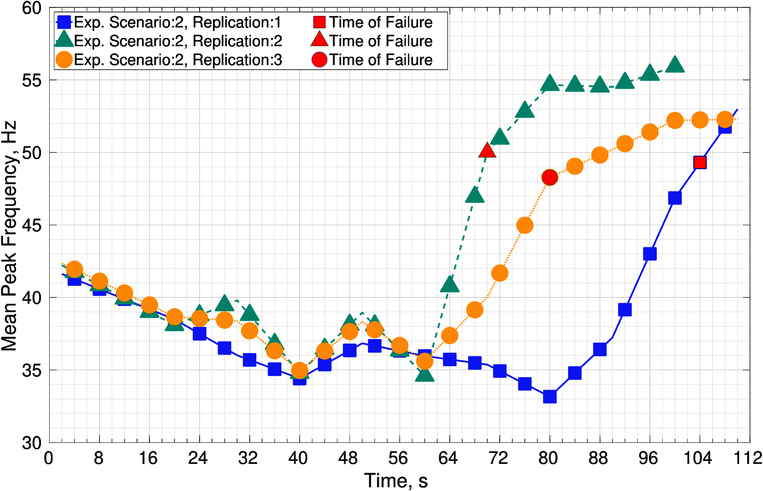
The computed mean peak frequencies for the 2nd experimental scenario.

In predictive maintenance, it is not sufficient to simply predict the class of future data as faulty or healthy. It is more important to accurately forecast the RUL so that the maintenance or other necessary actions can be taken well before the time of failure. Therefore, the problem in this study can be thought of as time series forecasting rather than a classification problem.

The computed mean peak frequency can be considered as a time series. These time series were obtained offline, that is, the calculation was done after the experiment was conducted. However, it is necessary to obtain a real-time computation for time series forecasting. Thus, the offline time series was considered as if it was obtained in real-time. This means that the time series updates itself iteratively with the new computed mean peak frequency value. As described in the methodology, the LSTM network forecasts the subsequent 5 mean peak frequency values using the last 7 values of the computed mean peak frequency as input. If one of these estimated values does not exceed the threshold value of 50 Hz, the time series is updated with the actual value of the first estimated mean peak frequency.

Figure 13 presents the forecasting results of all replications of the 3rd experimental scenario when one of the estimated mean peak frequency values exceeds the defined threshold. As a result, the RUL for the 1st, 2nd, and 3rd replications are 4 s, 10 s, and 10 s, respectively. In addition, the root mean square error (RMSE) between the estimated and the actual mean peak frequencies for the 1st, 2nd, and 3rd replications are 3.7142 Hz, 1.4831 Hz, and 1.3455 Hz, respectively.

Figure 13.

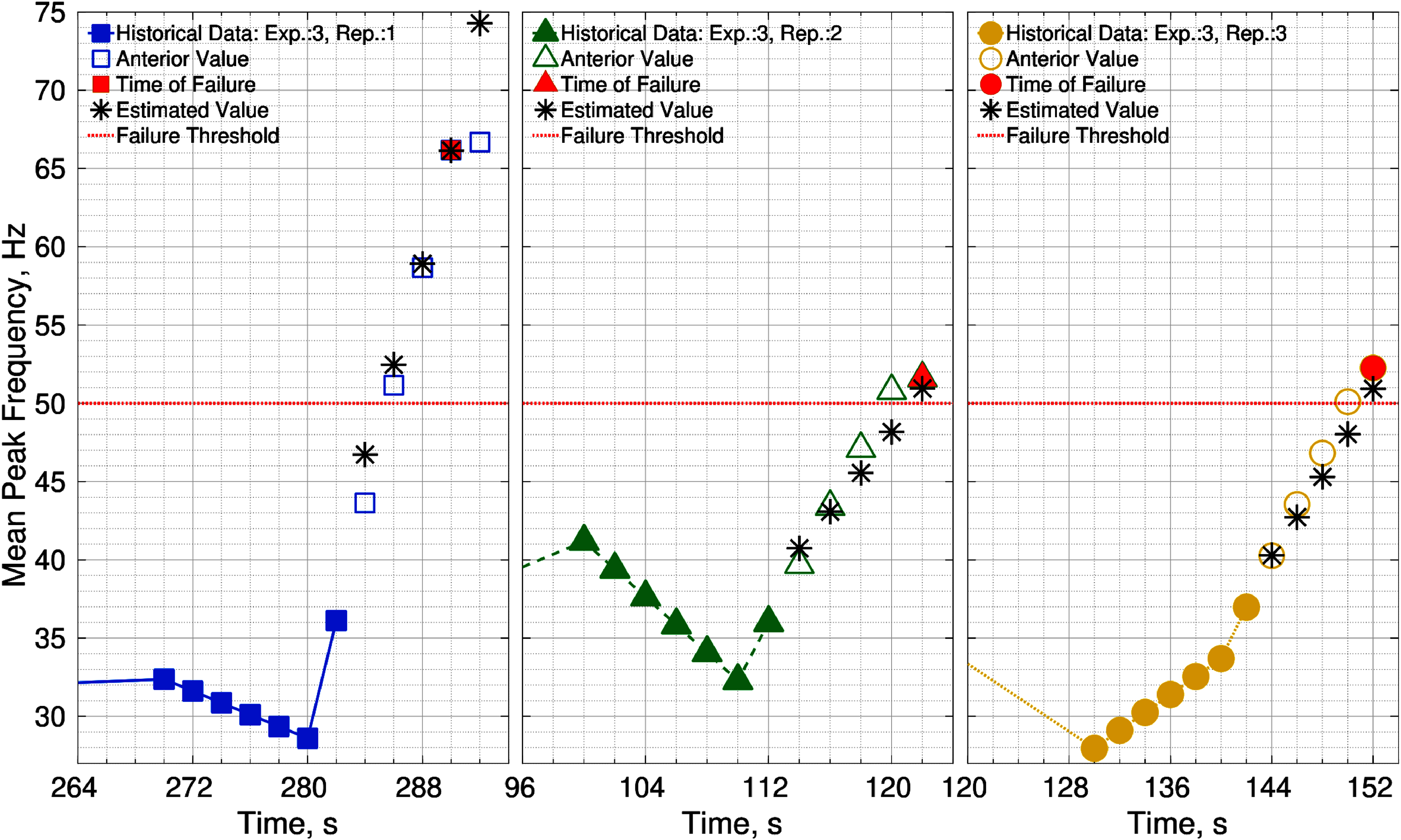
The estimated and actual mean peak frequencies for the 3rd experimental scenario.

In this study, the time window length between two mean peak frequencies is 2 s and the LTSM neural network always forecasts 5 mean peak frequency values. Thus, the maximum predictable time is 10 s. However, it can be expanded by increasing one of these two values. If the time window length was increased, it would be difficult to follow the sudden change in the time series. When the fault occurred, the estimated values would always be less than the actual values, resulting in an incorrect estimate as the estimated RUL would be longer than the actual value. On the other hand, if the estimated values were to increase, the accuracy would decrease and false alarms would occur because one of the estimated values might have exceeded the defined threshold.

Conclusions

This paper primarily used the mean peak frequency obtained from the time-frequency analysis to detect the RUL of a multi-rotor UAS. At first, the rotor vibration signals were segmented at 2-second window lengths and each segment was transformed from the time-domain into the time-frequency-domain. Then, the peak frequency was calculated for each time interval in the time-frequency-domain and the mean peak frequency was found by averaging these calculated peak frequencies.

The computed mean peak frequency values were considered as a time series and the LSTM neural network was used to estimate the values of the mean peak frequencies in the next 5 steps using the last 7 values of the computed mean peak frequency as input. If the estimated mean peak frequencies did not exceed the predefined threshold, the time series was updated with the actual value of the first predicted mean peak frequency. This way of updating the time series model captures instant trends. On the other hand, if one of the estimated peak frequencies exceeded the fault threshold, the time from estimation to fault occurrence was calculated as RUL.

The LSTM results demonstrated a strong agreement between the estimated and actual values of the mean peak frequencies. The RSME values for the 1st, 2nd, and 3rd replications were 3.7142 Hz, 1.4831 Hz, and 1.3455 Hz, respectively. The effectiveness of the proposed methodology was evaluated according to the results of the RUL estimation. In all the replications, RUL was computed before failure occurred and the maximum RUL was calculated as 10 s. The estimation depends on the selected time window length and the number of inputs and outputs of the LSTM neural network.

The subject of this research is a DJI M600, a commercial multi-rotor UAS designed not to fail. In particular, in order to make the wing structure frangible, a groove was deliberately cut in one of the wings, approximately 75% of the wing thickness. Experiment results demonstrated that the fracture was sharp and smooth and it was thought that the fracture occurred suddenly. Thus, it is difficult to forecast this sudden failure with a single feature and it is seen from the LSTM results that the forecast horizon is short. However, forecasting was still performed in the 3 cases before the failure. This information is incredibly useful for further work to broaden the forecasting horizon. The proposed feature, the mean peak frequency, performed well to detect degradation. During the healthy scenario, the mean peak frequency values were level at around 40 Hz at the first two throttle settings, as the throttle increased, they decreased up to 30 Hz because the controller of the UAS reduced the airframe vibration signals. On the other hand, during the faulty scenario, the mean peak frequency values showed a rapid increase from 40 Hz, which is the fundamental frequency, to 50 Hz as the time of failure approached, afterwards they increased slightly reaching 70 Hz at the end of the experiment. The ability to make a clear distinction between healthy and faulty operating conditions and the monotonic increase property after the failure shows that the mean peak frequency is a reliable feature in the detection of the failure.

One of the limitations of this research is to consider one flight operation (i.e. hover) to develop the RUL prediction method. In multirotor flight, the motor frequencies are constantly changing especially performing maneuvers. To increase the applicability of the developed method, real-world operations such as maneuvers or false alarms should be considered in future studies. Moreover, instead of a single feature, other features obtained in the time-domain, the frequency-domain, or a combination of these features can be utilized along with other modeling methods such as the extreme learning machine model to increase the forecasting horizon.

Footnotes

Acknowledgments

This study was partially supported by the Scientific and Technological Research Council of Turkey (TUBITAK) grant TUBITAK-2219, and partially by Innovation Fund Denmark (SafeEYE Project - no. 7049-00001). The funding parties have no role in the study design, data collection and analysis, decision to publish, or preparation of the manuscript.

CRediT Author Statement

Erkan Caner Ozkat: Conceptualization, Methodology, Formal analysis, Validation, Writing - original draft, review & editing. Oguz Bektas: Writing - review & editing. Micheal Juul Nielsen: Data curation, Writing - review & editing. Anders la Cour-Harbo: Funding acquisition, Resources, Supervision, Writing - review & editing.

Declaration of conflicting interests

The author(s) declared no potential conflicts of interest with respect to the research, authorship, and/or publication of this article.

Funding

The author(s) received no financial support for the research, authorship and/or publication of this article.

ORCID iDs

Erkan Caner Ozkat

Oguz Bektas

References

Kushleyev

MacAllister

Likhachev

. Planning for landing site selection in the aerial supply delivery. 2011 IEEE/RSJ International Conference On Intelligent Robots And Systems. 2011, pp. 1146–1153.

Thiels

Aho

Zietlow

et al. Use of unmanned aerial vehicles for medical product transport. Air Med J 2015; 34: 104–108.

Zahra

Buldan

Nazaruddin

et al. Predictive maintenance with neural network approach for UAV propulsion systems monitoring. 2021 American Control Conference (ACC). 2021, pp. 2631–2636.

Bondyra

Gasior

Gardecki

et al. Fault diagnosis and condition monitoring of UAV rotor using signal processing. 2017 Signal Processing: Algorithms, Architectures, Arrangements, And Applications (SPA). 2017, pp. 233–238.

Marino

Fisher

Clothier

et al. An evaluation of multi-rotor unmanned aircraft as flying wind sensors. Int J Micro Air Vehicles 2015; 7: 285–299.

Bektash

Cour-Harbo

. Vibration Analysis for Anomaly Detection in Unmanned Aircraft. 2020 Annual Conference Of The Prognostics And Health Management Society. 2020.

Williams

. A Summary of Unmanned Aircraft Accident/Incident: Data Human Factors Implications. (Civil Aerospace Medical Institute, Federal Aviation Administration, 2004, 12).

Susini

. A technocritical review of drones crash risk probabilistic consequences and its societal acceptance. Lnis 2015; 7: 27–38.

Che Man

Haoliang

Low

. Crash area estimation for ground risk of small unmanned aerial vehicles due to propulsion system failures. SCITECH 2022 Forum. 2022, p. 1506.

10.

Franco

Góes

. Failure analysis methods in unmanned aerial vehicle (UAV) applications. Proceedings Of COBEM 2007 19th International Congress Of Mechanical Engineering. 2007.

11.

Ghasri

Maghrebi

. Factors affecting unmanned aerial vehicles’ safety: a post-occurrence exploratory data analysis of drones’ accidents and incidents in Australia. Saf Sci 2021; 139: 105273.

12.

Cour-Harbo

. Mass threshold for ‘harmless’ drones. Int J Micro Air Vehicles 2017; 9: 77–92.

13.

Unija

. Commission implementing regulation (EU) 2019/947 of 24 May 2019 on the rules and procedures for the operation of unmanned aircraft. Off J Eur Union 2019; 152: 45–71.

14.

Sándor

Pusztai

. Certification of unmanned aircraft systems from product safety to type certificate–A review about the operation of the EU safeguard processes. Acta Tech Jaurinensis 2021; 15: 36–46.

15.

Bektash

Pedersen

Gomez

et al. Automated emergency landing system for drones: SafeEYE Project. 2020 International Conference On Unmanned Aircraft Systems. 2020, pp. 1056–1064.

16.

Paolanti

Romeo

Felicetti

et al. Machine learning approach for predictive maintenance in Industry 4.0. 2018 14th IEEE/ASME International Conference On Mechatronic And Embedded Systems And Applications (MESA). 2018, pp. 1–6.

17.

Dalzochio

Kunst

Pignaton

et al. Machine learning and reasoning for predictive maintenance in Industry 4.0: Current status and challenges. Comput Ind 2020; 123: 103298.

18.

Selcuk

. Predictive maintenance, its implementation and latest trends. Proc Ins Mech Eng, Part B: J Eng Manuf 2017; 231: 1670–1679.

19.

Leukel

González

Riekert

. Adoption of machine learning technology for failure prediction in industrial maintenance: A systematic review. J Manuf Syst 2021; 61: 87–96.

20.

Pech

Vrchota

Bednář

. Predictive maintenance and intelligent sensors in smart factory. Sensors 2021; 21: 1470.

21.

Nguyen

Medjaher

. A new dynamic predictive maintenance framework using deep learning for failure prognostics. Reliab Eng Syst Saf 2019; 188: 251–262.

22.

Ozkat

. The comparison of machine learning algorithms in estimation of remaining useful life. IX Int Maint Technol Congress 2019; 614–619.

23.

Ayvaz

Alpay

. Predictive maintenance system for production lines in manufacturing: a machine learning approach using IoT data in real-time. Expert Syst Appl 2021; 173: 114598.

24.

Mao

Tang

et al. Predicting remaining useful life of rolling bearings based on deep feature representation and long short-term memory neural network. Adv Mech Eng 2018; 10: 1687814018817184.

25.

Zheng

. Predicting remaining useful life based on Hilbert–Huang entropy with degradation model. J Electr Compu Eng 2019; 2019: 1–11.

26.

Ragab

Elhefnawy

Ouali

. Artificial Intelligence-Based Survival Analysis For Industrial Equipment Performance Management.2022 Annual Reliability And Maintainability Symposium (RAMS), 1–7.

27.

Goebel

. Degradation modeling and remaining useful life prediction of aircraft engines using ensemble learning. J Eng Gas Turbine Power 2019; 141: 041008.

28.

Liu

Song

Niu

et al. A generalized cauchy method for remaining useful life prediction of wind turbine gearboxes. Mech Syst Signal Process 2021; 153: 107471.

29.

Schwartz

Jiménez

Vingerhoeds

et al. An unsupervised approach for health index building and for similarity-based remaining useful life estimation. Comput Ind 2014; 141: 103716.

30.

Yan

Gao

. Multi-scale enveloping spectrogram for vibration analysis in bearing defect diagnosis. Tribol Int 2021; 42: 293–302.

31.

Jiménez

Schwartz

Vingerhoeds

et al. Towards multi-model approaches to predictive maintenance: a systematic literature survey on diagnostics and prognostics. J Manuf Syst 2020; 56: 539–557.

32.

Cakir

Guvenc

Mistikoglu

. The experimental application of popular machine learning algorithms on predictive maintenance and the design of IIoT based condition monitoring system. Comput Ind Eng 2021; 151: 106948.

33.

Kammerer

Gaust

Küstner

et al. Motor classification with machine learning methods for predictive maintenance. IFAC-PapersOnLine 2021; 54: 1059–1064.

34.

Peng

Dong

Zuo

. Current status of machine prognostics in condition-based maintenance: a review. Int J Adv Manuf Technol 2010; 50: 297–313.

35.

Susto

Schirru

Pampuri

et al. Machine learning for predictive maintenance: a multiple classifier approach. IEEE Trans Ind Inf 2014; 11: 812–820.

36.

Ahmed

Carpitella

Certa

. An integrated methodological approach for optimising complex systems subjected to predictive maintenance. Reliab Eng Syst Saf 2021; 216: 108022.

37.

Cheng

Chen

et al. Data-driven predictive maintenance planning framework for MEP components based on BIM and IoT using machine learning algorithms. Autom Constr 2020; 112: 103087.

38.

Sajid

Haleem

Bahl

et al. Data science applications for predictive maintenance and materials science in context to Industry 4.0. Materials Today: Proceedings 2021; 45: 4898–4905.

39.

Carvalho

Soares

Vita

et al. A systematic literature review of machine learning methods applied to predictive maintenance. Comput Ind Eng 2019; 137: 106024.

40.

Popescu

Aiordachioaie

Culea-Florescu

. Basic tools for vibration analysis with applications to predictive maintenance of rotating machines: an overview. Int J Adv Manuf Technol 2022; 118: 2883–2899.

41.

Oliveira

Magalhães

Cunha

et al. Vibration-based damage detection in a wind turbine using 1 year of data. Struct Control Health Monit 2018; 25: 1–22.

42.

Shin

Han

Rhee

. AI-assistance for predictive maintenance of renewable energy systems. Energy 2021; 221: 119775.

43.

Nayana

Geethanjali

. Analysis of statistical time-domain features effectiveness in identification of bearing faults from vibration signal. IEEE Sens J 2017; 17: 5618–5625.

44.

Saidi

Ali

Bechhoefer

et al. Wind turbine high-speed shaft bearings health prognosis through a spectral kurtosis-derived indices and SVR. Appl Acoust 2017; 120: 1–8.

45.

Elasha

Shanbr

et al. Prognosis of a wind turbine gearbox bearing using supervised machine learning. Sensors 2019; 19: 3092.

46.

Ciabattoni

Ferracuti Freddi

et al. Statistical spectral analysis for fault diagnosis of rotating machines. IEEE Trans Ind Electron 2017; 65: 4301–4310.

47.

Teng

Zhang

Liu

et al. Prognosis of the remaining useful life of bearings in a wind turbine gearbox. Energies 2016; 10(1): 32.

48.

Teng

Han

et al. A robust model-based approach for bearing remaining useful life prognosis in wind turbines. IEEE Access 2020; 8: 47133–47143.

49.

Kumar

Manjunath

. Vibration signal analysis using time and time–frequency domain. 2017 IEEE International Conference on Power, Control, Signals and Instrumentation Engineering (ICPCSI). 2017, pp.1808–1811.

50.

Ali

Saidi

Harrath

. Online automatic diagnosis of wind turbine bearings progressive degradations under real experimental conditions based on unsupervised machine learning. Appl Acoust 2018; 132: 167–181.

51.

Fulop

Fitz

. Bearing fault diagnosis and prognosis using data fusion based feature extraction and feature selection. Measurement 2022; 188: 110506.

52.

Yan

Gao

. Multi-scale enveloping spectrogram for vibration analysis in bearing defect diagnosis. Tribol Int 2009; 42: 293–302.

53.

Bouabdallah

Murrieri

Siegwart

. Design and control of an indoor micro quadrotor. 2004 IEEE International Conference on Robotics and Automation. 2004, pp.4393–4398.

54.

Pourpanah

Zhang

et al. Anomaly detection and condition monitoring of UAV motors and propellers. 2018 IEEE Sensors. 2018, pp.1–4.

55.

Che

Wang

et al. Combining multiple deep learning algorithms for prognostic and health management of aircraft. Aerosp Sci Technol 2019; 94: 105423.

56.

Shenoi

. Introduction to digital signal processing and filter design. New Jersey: John Wiley & Sons, 2005.

57.

Mitra

Kuo

. Digital signal processing: A computer-based approach. Vol. 2. New York: McGraw-Hill, 2006.

58.

Fulop

Fitz

. Algorithms for computing the time-corrected instantaneous frequency (reassigned) spectrogram, with applications. J Acoust Soc Am 2006; 119: 360–371.

59.

Hochreiter

Schmidhuber

. Long short-term memory. Neural Comput 1997; 9: 1735–1780.

60.

Joy

Rana

Gupta

et al. Hyperparameter tuning for big data using Bayesian optimisation. 23rd International Conference On Pattern Recognition (ICPR). 2016, pp.2574–2579.

61.

Chaudhuri

D Alkan

. A hybrid extreme learning machine model with harris hawks optimisation algorithm: an optimised model for product demand forecasting applications. Appl Intell 52: 11489–11505.

62.

Sejdić

Djurović

Jiang

. Time–frequency feature representation using energy concentration: An overview of recent advances. Digit Signal Process 2009; 19: 153–183.

A data-driven predictive maintenance model to estimate RUL in a multi-rotor UAS

Abstract

Keywords

Introduction

Literature review

Methodology for RUL estimation

Data preprocessing

Feature extraction

RUL estimation

Testing and results

Generation of vibration data

Implementation of the proposed methodology

Conclusions

Footnotes

Acknowledgments

CRediT Author Statement

Declaration of conflicting interests

Funding

ORCID iDs

References