Sage Journals: Discover world-class research

Abstract

As small Uninhabited Aerial Vehicles (sUAS) increase in popularity, computational analysis is increasingly being used to model and improve their performance. However, although propeller performance is one of the primary elements in modelling an aircraft, most manufacturers of propellers for this size of vehicle do not publish geometric information for the propeller. The lack of available geometric data makes simulation of propeller aerodynamics challenging. While techniques exist to accurately extract the 3D geometry of a propeller, these methods are often very expensive, time-consuming, or labor intensive. Additionally, typical 3D scanning techniques produce a 3D mesh that is not useful for techniques such as Blade Element Theory (BET), which rely on knowledge of the 2D cross sections along the propeller span. This paper describes a novel workflow to produce point clouds using readily available photo equipment and software and subsequently extract airfoil and propeller blade parameters at specified stations along the propeller span. The described process can be done with little theoretical knowledge of photogrammetry and with minimal human input. The propeller geometry generated is compared against results of established methods of geometry extraction and good agreement is shown.

Keywords

Photogrammetry drone Propellers airfoil fitting propeller simulation point-to-Plane

Introduction

The increasing popularity of small Uninhabited Aerial Systems (sUAS) in various fields and applications has made them a subject of academic interest. Multirotors or, colloquially, “drones” are seeing use in aerial photography, scientific surveying, law enforcement, and even delivery. As the name implies, these vehicles fly using multiple propellers to provide the lift required to counteract gravity as well as to maneuver. The ubiquity of drones means that aerodynamic analysis of propellers in these conditions is important to determine the efficiency of a design, and to characterize its dynamics.

Existing simulation methods can accomplish both these tasks to varying degrees of accuracy and complexity. The most basic analysis possible is the classical actuator disc model.¹ The actuator disc model may capture the general effects of a rotor on the surrounding fluid, but doesn’t capture the specifics of a particular propeller. This analysis method provides a basic relation between thrust, and the momentum and energy in the flow, but says little about how that relates to a propeller rotation speed necessary for a controls formulation nor how the airflow may interact with other portions of the drone. Simulation methods that do consider the propeller geometry are Blade Element Theory (BET) or Blade Element Momentum Theory (BEMT).² These predict the propeller performance by considering each section of the blade in a psuedo 2D manner. Another method is the Vortex Particle Method,³ which has the advantage of numerically propagating the vorticity from the propeller, allowing for a prediction of the interaction between the propeller and other structures on the aircraft in a grid free manner. Accurately shedding vortex particles from the propeller blades requires knowledge of the blade geometry to calculate the lift distribution along the blade span. There are also Computational Fluid Dynamics (CFD) approaches involving mesh-based Reynolds-averaged Navier-Stokes (RANS) simulations.⁴ While this is the most comprehensive simulation method, it is computationally expensive. Results from one case at a particular rotation speed, freestream speed, etc. are not necessarily transferable to a different case, making studies inconvenient if one desires to study a multitude of cases. One commonality of all the aforementioned methods, except for the disk actuator method, is that the propeller geometry must be known in some form in order to simulate the aerodynamics properly. Furthermore, while mesh-based simulations might be able to accept a diversity of 3D model formats for the propeller, the lower-order methods require a description of the propeller either geometrically or aerodynamically at stations along the blade span.

With the popularity of computational methods for analysis and performance improvement, accurate 3D models of component geometry are more critical than ever. However, most popular manufacturers of propellers for this size of vehicle do not provide detailed geometric specifications for their propellers and instead only provide the diameter and pitch, a simple measure of the blade inclination. Some suppliers publicly provide design information beyond these metrics,⁵ but many do not. A lack of published geometry necessitates reverse engineering this data. While databases do exist of some of these efforts,⁶ they do not keep pace with the wide range of available products for drone enthusiasts and researchers today. There is a clear dearth of accurate and accessible propeller geometry data for researchers. While there are existing techniques for the accurate extraction of propeller geometry, they are often expensive, time consuming, destructive, or some combination thereof. This work addresses the inaccessibility of propeller geometry by outlining a non-destructive technique that requires little specialized equipment, is comparatively rapid compared to similar techniques, and requires little human input. This method is shown to produce geometric data that, when simulated, produced thrust values within 10% of experimental results.

Requirements and review of existing methods

While various 3D scanning technologies exist, there is always a trade-off among speed, cost, and accuracy. To consider available technologies, we first consider what level of accuracy is needed. Ideally, the measured geometry of the airfoil would be at a resolution such that we could correctly distinguish between two airfoils within the same family. Taking the NACA four digit series for reference,⁷ the last two digits represent the maximum thickness of the airfoil in percentage of the airfoil’s chord. Resolving the cross section with sufficient accuracy to differentiate one four digit airfoil from another, requires ordinates of the airfoil of the propellers cross section to be accurate to within one percent of the station’s chord. For the propellers examined in the paper with blade chords of roughly 10 mm, this corresponds to a thickness accuracy of less than 0.1 mm.

A classical method of surface extraction is with a Coordinate Measuring Machine (CMM).⁸ A computer-controlled CMM can measure geometry to very high precision (on the order of microns in some cases⁹), but the process is slow. As a contact based method of measurement, the process may also be sensitive to the flexibility of the part. This displacement can be unacceptably large dependant on the material and size of the propeller and may necessitate an application specific CMM.¹⁰ The hardware required for these scans can also be prohibitively expensive. The probe component alone can cost thousands of dollars,¹¹ far more than might be worthwhile for just one step in a larger process of simulation.

Laser scanning is a similar, more mobile technology suited for the problem. By projecting a slender line onto an object and viewing the resulting contour from a camera with known relative position, the observed contour can be interpreted to create a virtual body. A system capable of measuring the geometry to sufficient accuracy is quite costly however, given the specific application.¹² A popular, low cost, technique for small Uninhabited Aerial System (sUAS)-scale propellers is to cast the propeller in resin, cut the propeller into sections and scan the faces on a conventional document scanner.^13,14 This has the advantage of having high dimensional accuracy and requiring little specialized equipment, but is time consuming and destroys the propeller. This method of extraction is used for comparison later in this work. Additional low cost propeller-specific techniques include matching the section using a piece of solder¹⁵ which is still time consuming, and measuring the properties using a pitch gauge setup¹⁶ which is simple and quick, but requires a specialized tool and does not convey the airfoil section of the propeller.

Photogrammetry is a potential avenue to sidestep the deficiencies of the preceding methods. Photogrammetry can require very little specialized equipment and theoretically has the requisite accuracy; close range photogrammetry has a potential measurement precision of 1:500,000 relative to the largest object dimension.¹⁷ Photogrammetry has been applied in the field of aerodynamic study previously. One work looks at the accuracy of the method and uses it to quantify wing aeroelastic deflection.¹⁸ Another that successfully extracts a surface from a flapping dragonfly inspired wing uses the surface texture.¹⁹ There exists previous work to extract specifically propeller geometry using photogrammetry. One work²⁰ details a high quality method using the commercial V-STARS system for marine propeller applications. At the time, the system appeared to require specific patterns of markers to be applied to the surface of the object to be measured, a clear inconvenience for something the size of drone scale propellers. A more recent paper¹⁰ compares various scanning technologies, again for a marine propeller. The paper includes photogrammetry in the comparison, and uses a now defunct commercial package, Photomodeler Scanner,²¹ as well as a no longer extant online service, ARC 3D.²² This study also mentions previous work²³ as a basis for some of the work done where the authors developed their own photogrammetry process for evaluation of marine propellers and ship hulls. Another work compares the relative deformation of two blades of a propeller using photogrammetry.²⁴ This work however still uses targets applied to the surface and only uses the data to compare the geometry between blades rather than extract their base geometry. Lastly, a recent paper¹⁴ aims to achieve very similar goal to the work outlined here, but takes a different approach to the physical modeling of the blade. In that work, a T-spline surface is fit to the photogrammetry mesh, and the result deviates significantly from the true blade section collected by slicing the propeller. Sections illustrated in this work show a rounded trailing edge in contract to the sharp edge that one might expect from an airfoil section. Furthermore, a surface description of the propeller might be appropriate for a mesh-based simulation, but would require additional processing before it could be used in a lower order simulation methods such as BET.¹ Summarizing the results of the literature survey in the previous paragraph, existing work often used a commercial photogrammetry systems or software, required the application of specific markers to the propeller surface, or did not reconstruct the propeller in a convenient format. While commercial off the shelf photogrammetry systems are available, they and other 3D scanning systems are costly. There is a lack of a complete, start-to-finish methodology for those wanting to produce accurate propeller geometry using photogrammetry.

Contribution of the work

The preceding survey of existing methods highlights both the importance of accurate geometry for modern simulation, as well as the inadequacy or inaccessibility of existing technologies to provide this in a convenient manner. The contributions of this work are as follows. First, a set of systematic guidelines is presented for photo collection to reliably produce a dense and accurate pointcloud of a propeller using photogrammetry. Second, an algorithm for alignment, scaling and feature extraction of the pointcloud that requires minimal human input is presented. Third, in contrast with existing work, we present a complete, end-to-end pipeline uniting all the steps which, to the authors’ knowledge, has not been done before. Fourth, the objective of this work is to present the technique with sufficient information to function as a tutorial for the community. This methodology is outlined in Figure 1.

Figure 1.

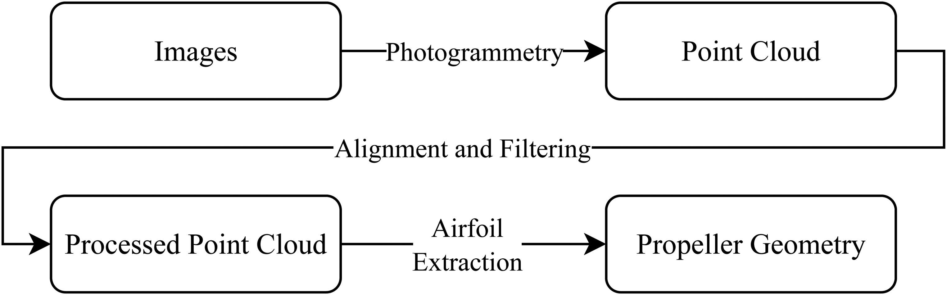
Flowchart of propeller property extraction process.

Furthermore, while this process was conceived and has been optimized for use with propellers, it is also applicable to adjacent problems. The process could be easily applied to a wing on a UAV with virtually no modifications, and other shapes could be analyzed using the same algorithms if one changed the shape parametrization in the Airfoil Extraction step.

Portions of this work were previously presented at the American Physical Society annual Division of Fluid Dynamics meeting.²⁵ Progression on this work since then has included improvements in the manual fitting functionality, implementation of the automatic fitting algorithm for coordinate system alignment, and the simulation of the propeller performance as well as its comparison with experimental data. General improvements to the code have also occurred since then to implement these new features and make the process more user-friendly.

Organization

The rest of the paper will follow the ordering shown in Figure 1 and is organized as follows. Section Photogrammetry Setup for Propellers describes the process by which the point cloud is generated. This includes techniques in the photo collection phase that will improve the quality of the point cloud and a description of the photogrammetry software. Section Point Cloud Post-Processing describes the process to align the information to a useful coordinate system, and filter the data. Section Propeller Property Extraction describes how the propeller properties are extracted from the point cloud. Section Photogrammetry Results then takes the results of using the methodology on several propellers and evaluates their accuracy. Section Propeller Force Prediction takes the computed geometry and simulates their performance, comparing the results against experimental data. As the techniques described in this work use math from several different fields, nomenclature will be described in specific sections.

Photogrammetry setup for propellers

Generating a quality point cloud is the foundation of this process. The subsequent sections describe techniques relevant to this process that help a user produce quality geometric data for drone propellers.

Available photogrammetry software is now powerful and user friendly enough that a high quality point cloud can be produced with very little knowledge of photogrammetry and with some consideration for the photos taken. The software primarily used in this work to produce the point cloud is COLMAP,^26,27 a general-purpose Structure-from-Motion (SfM) and Multi-View Stereo (MVS) software. While the directions provided in this work reflect the choice of software, many alternative free photogrammetry softwares are available such as Meshroom,²⁸ MicMac,²⁹ Multi-View Environment,³⁰ OpenMVG,³¹ Regard3D,³² and VisualSFM.^33–35 As long as the choice of photogrammetry software can produce geometric data that can be edited and manipulated, the user can proceed to use the described techniques to align and filter data. Finally, the described algorithm can be used to fit and extract the relevant the geometric parameters describing the propeller.

Photo collection

A number of simple considerations, taken into account when photographing the propeller, help the photogrammetry algorithms produce a sufficiently dense point cloud. The techniques described in this section were found to significantly improve the results of the photogrammetry. In this work, image sets were mainly taken with a Sony Rx 10 IV which has a 21 Megapixel sensor. However, it was found that the images from the camera of a modern (at the time of writing) smartphone with a 16 Megapixel sensor could also produce quality results. While higher quality images lead to a better quality point cloud, the required quality of image was not studied in depth. Quantifying image quality can be subjective based on the mechanical limitations of the camera, or image focus and other factors beside pure resolution. Furthermore, the image quality of the camera on a typical smartphone is already sufficient for this application and is generally expected to increase. The setup for how the images are taken, as described in this section, was found to have a much larger influence on the quality of the photogrammetry.

Initially, it was attempted to simply take a video of the propeller and extract still frames for analysis. While this technique had some success, the results had lower resolution than desired. Generally, regardless of if the camera was moved and the object held in place or vice versa, there were issues with focus and motion blur. Any built in video compression would also detract from the still frame quality. Extracting useful frames from the camera, which was supposed to improve the ease of collecting a data set, instead became laborious as frames with minimal blurring were needed to produce a usable point cloud.

It was instead elected to keep the camera at a fixed position with fixed zoom and focus and simply rotate the propeller to extract the point cloud. Though initially a turn-table connected to a servo was constructed to rotate the propeller automatically, placing the propeller on a manually-rotated swivel chair was found to be a better and faster solution. The chair is assumed to remain stationary, however small translations will not impact the results provided the propeller remains in the field of view and acceptable depth of field of the camera.

To help facilitate this, the propeller is placed as near as possible to the axis of rotation of the chair and remains in the same position relative to the camera. By keeping the parameters of the camera such as focal length, zoom, aperture, and ISO constant, there is no need for adjustment between photos as the propeller is rotated, shortening the data collection process. Additionally, fixed camera settings carry the added advantage of simplifying the camera characterization problem, reducing it to just one set of settings for the session rather than a set of unknown characteristics for each image. Although the object would ideally be under consistent lighting conditions throughout image collection, sufficiently diffuse lighting and small enough changes between images still allow features to be recognized effectively in the software.

It was found that roughly 50 images, evenly spaced in a circular pattern around the propeller were sufficient to produce a good quality point cloud. This number was chosen primarily because of the limitations of the photogrammetry process. 50 was the number of images that resulted when photos were taken with a small enough angular displacement for the software to reliably find a solution to the camera positions relative to one another while having photo coverage of the entire propeller. This corresponds to between a 5 to 10 degree angular displacement between shots.

In order to properly extract the propeller surface geometry, there need to be features that can be recognized and correlated between images. Features that are well recognized are typically regions of high color or brightness contrast. Propellers sold for sUAS applications are often a single color and glossy, preventing good feature recognition on their surfaces. To improve feature acquisition, a small variety of patterns were drawn on the propeller surface with a marker of a contrasting color. For example, one of the propellers used in this work was made of a glossy orange plastic, so black marker stood out well and the application of a layer of ink was deemed thin enough such that it would likely not impact the geometry of the propeller or its performance. The patterns drawn on the propeller were a random, medium density speckle pattern as well as a loose grid. The change in quality of the point cloud is clearly visible in different regions of the propeller corresponding to these patterns. The hand-drawn grid was sufficient to produce good results. As seen in Figure 2, the effect of the pattern on the point cloud is clear. In region A, the pattern drawn on the hub cylinder wall produces a denser point cloud than that produced at region B, where the lack of pattern has resulted in a gap in the cloud. Likewise, the point cloud density appears adequate around each of the drawn dots in region C, but the sparseness of the dots means that there are still gaps in the surface. In contrast, the grid drawn in region D results in a much higher density point cloud. While a sufficiently dense dot pattern can create a useable point cloud, the authors found the grid pattern to be easier to draw.

Figure 2.

Comparison of Point Cloud Resolution of different regions on the propeller based upon surface pattern. (a) Sample Image and (b) Photogrammetry Point Cloud.

Also note that in the point cloud in Figure 2b, there are a number of points clustered around the edges of the propeller with the color of the background. A method of addressing these is described in section Color Based Filtering.

An alternative to a hand-drawn pattern is a spray painted speckle pattern, similar to what is used in Digital Image Correlation processes. With proper application, the underlying color of the propeller is irrelevant, and the entire surface will have a good quality pattern. It was found that the addition of paint will add roughly 0.025–0.04 mm to a surface. Disadvantages are that the process may impact the propeller’s usability on vehicles. Potential effects are unbalancing the propeller and interactions between the surface boundary layer and the paint. Some paints also contain solvents, such as acetone, that could potentially damage the propeller, rendering it structurally unsound.

In addition to applying a pattern to the propeller surface, it was also found important to have a clear, identifiable pattern in the background of the image; a recognizable pattern solely on the object was found to be insufficient. The common features between images provided by the background are used to estimate the position of the camera, which is a critical part of the reconstruction process. A checkerboard pattern, even non-planar and out of focus was found to provide a good reference.

The challenge, though, is that the background needs to move with the propeller. As the photogrammetry software relies on the assumption of a static scene and a moving camera, having the reverse can cause problems if the region of interest is moved relative to the camera but background elements remain fixed. As the software has no inherent way to identify background elements that are not relevant to the scene, the camera needs to either be set up to exclude these elements, or the images need to be filtered with a mask. As seen in the setup shown in Figure 3 this objective is achieved by having the checkerboard pattern rotate with the object. The camera was positioned and the zoom set such that the propeller and checkerboards occupied as much of the field of view as possible, minimizing the effect of the background. This constraint also drove the vertical placement of the camera relative to the propeller. Placing the plain, featureless floor in the background of the shot by facing the camera downwards helped to prevent any features being incorrectly recognized for the camera position calculation.

Figure 3.

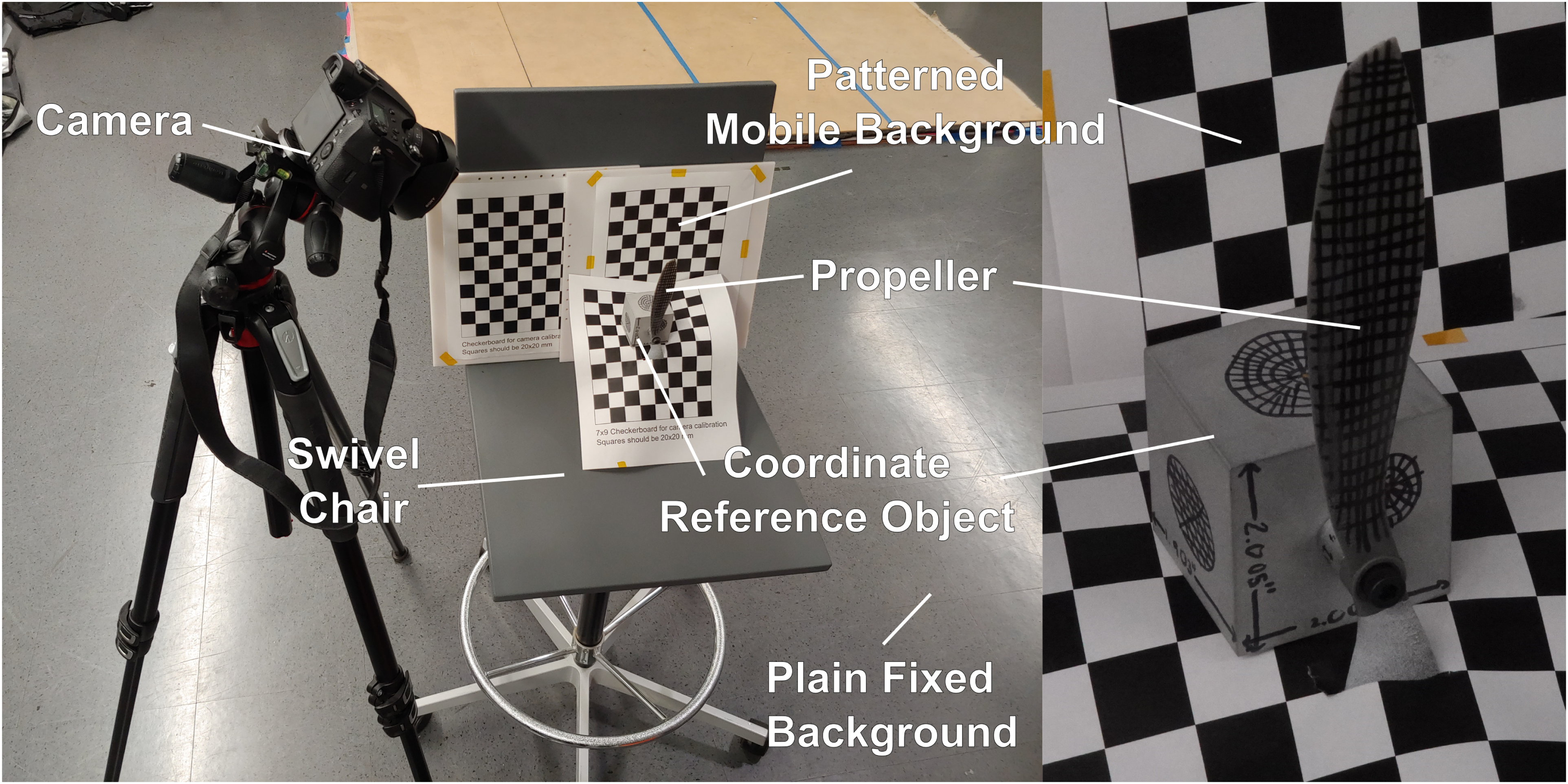
Experimental Setup.

The application of the described suggestions should reliably produce viable image sets and improve output quality. A summary of these guidelines can be seen in Table 1.

Table 1.

Summary of photo collection guidelines.

Guideline	Effect
Propeller on rotating surface, near axis of rotation	Propeller moves rather than camera, allowing for fixed camera settings
Fixed camera settings during collection	Reduces complexity of photogrammetry problem, speeds up collection by removing focusing time
Maximize propeller in field of view	Reduces extraneous points in point cloud, maximizes resolution on the propeller, minimizes stationary background in the frame
High contrast background patterns moving with the propeller	Improves likelihood of correctly calculating camera position, allowing for that image to be used in the reconstruction
Dense, high-contrast pattern on propeller surface	Increases feature recognition on the propeller surface and increases point cloud density
Textured reference object attached to the propeller	Provides coordinate system and scale reference for the point cloud

Point cloud generation

In order to reconstruct the 3 dimensional data from the set of captured images, we use a photogrammetry software. COLMAP, the software used in this work, features sparse and dense reconstruction processes. It is expected that a similar procedure can be carried out for any photogrammetry software. The sparse reconstruction process identifies common features within each photo and attempts to extract the camera properties and position for each photo. Using the same camera settings for each shot and taking photos in a sequential manner and selecting the relevant options to take advantage of this improves the success rate of the sparse reconstruction process. A successful reconstruction can be seen in Figure 4. The camera positions calculated appear to all lie on the same circle, which is consistent with how the pictures were taken. The view angles are also relatively dense, meaning that all the relevant surfaces of the propeller will get good photo coverage. One of the indicators of a good image set that the authors identified is that the software identifies the relative locations of the camera for all the images in the set without discarding any. This step of the reconstruction takes little time, on the order of minutes, so one can quickly determine if the image set collected is of sufficient quality using this criteria.

Figure 4.

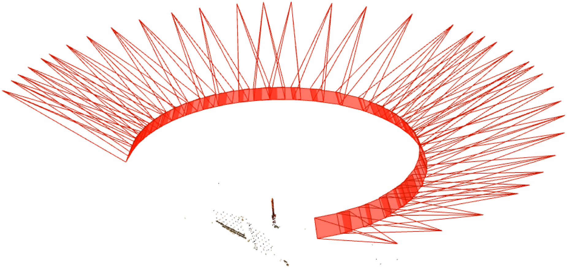
Graphical representation of estimated camera positions produced by COLMAP.

Once the sparse reconstruction is completed, the dense reconstruction is run on the data. This software requires a computer with a GPU to perform the dense point cloud reconstruction. On a computer with an Nvidia RTX 970 the reconstruction process takes about 1 hour for a set of roughly 50 images. Additional images may improve the resolution, but will also take additional computational time. Given that reconstruction time on the order of an hour produced a point cloud that was considered to be of sufficient density, little study was devoted to comparing size of the image set, reconstruction time, and point cloud quality. Once the dense reconstruction process is complete, the point cloud can be exported for the subsequent manipulations.

Point cloud post-processing

The raw data produced from photogrammetry needs to be prepped before it can be interpreted. The following sections describe how the data are aligned and cleaned.

Point cloud alignment

Initially, the point cloud is described in a coordinate system that is determined by the photogrammetry algorithm, and is functionally random in orientation and scale. To produce useful parameters, we must first orient the data into a more useful coordinate system and scale it accurately. In this work, we choose to place the coordinate system origin at the center of the propeller hub and orient the blade such that the propeller’s thrust axis is aligned with the positive X-axis and the blade of interest is aligned with the positive Z-axis. The Y-axis is then chosen to form a right handed coordinate system. An illustration of this is shown in Figure 5. The correct scaling is determined using a reference from the scene that is of known length.

Figure 5.

Coordinate system for the propeller.

Manual alignment process

Manual coordinate system alignment is possible, but relies on visually determining whether parts are at the correct angles. To do this, we select two points, one near the blade tip and one near the blade root to use as our first pass at a Z basis vector. The data is then transformed and displayed, and rotation corrections are applied to orient the data as desired.

The specifics of the process are the following: choose two initial points $x_{a}$ and $x_{b}$ from the point cloud such that $x_{a}$ is near the root of the blade and $x_{b}$ to be near the tip of the blade.

v_{1} = \frac{x_{b} - x_{a}}{‖ x_{b} - x_{a} ‖}

(1)

v_{2} = v_{1} \times i_{x}

(2)

v_{3} = v_{1} \times v_{2}

(3)

i_{x}

is the unit vector in the global

X

direction, simply to provide a starting point to produce a vector orthogonal to

\vec{v_{1}}

. The orthonormal basis describing the propeller coordinate system in the initial point cloud coordinate system is described by the matrix

A = [v_{2} v_{3} v_{1}]

(4)

We then apply rotations using an XYZ rotation sequence to visually correct the misalignment. Finally, the data is scaled to match the physical dimensions of the propeller. The scaling is done by identifying an object with known size within the point cloud, and linearly scaling all the coordinates until the size of the reference object in the point cloud reflects reality. In the data collected, the calibration pattern with a checkerboard of known size was used as a reference for length. Lastly, we shift the point cloud such that the origin is coincident with the center of the propeller hub. The complete transformation from points in the raw point cloud coordinate system

X_{raw}

to points in our chosen working coordinate system

X_{working}

X_{working} = S_{Length} (R_{x} R_{y} R_{z} (A X_{raw}) - X_{0})

(5)

\begin{aligned} R_{x} = [\begin{matrix} 1 & 0 & 0 \\ 0 & \cos (θ_{X}) & - \sin (θ_{X}) \\ 0 & \sin (θ_{X}) & \cos (θ_{X}) \end{matrix}] \\ R_{y} = [\begin{matrix} \cos (θ_{Y}) & 0 & \sin (θ_{Y}) \\ 0 & 1 & 0 \\ - \sin (θ_{Y}) & 0 & \cos (θ_{Y}) \end{matrix}] \\ R_{z} = [\begin{matrix} \cos (θ_{Z}) & - \sin (θ_{Z}) & 0 \\ \sin (θ_{Z}) & \cos (θ_{Z}) & 0 \\ 0 & 0 & 1 \end{matrix}] \end{aligned}

where

S_{Length}

is the scaling factor used, calculated as

L_{true} / L_{raw}

L_{raw}

is the length of a reference object or distance within the point cloud and

L_{true}

is the analogous true distance in a chosen unit system.

X_{0}

is the coordinate of the desired origin within the original raw coordinate system.

Automatic alignment with a known reference object

If available, a more convenient alternative to visual point cloud orientation is to include a reference object of known dimensions and orientation relative to the propeller. In this work, a rectangular prism was machined for this purpose. The prism was then bead blasted to a matte finish so reflections would not interfere with the photogrammetry and patterns were drawn on the faces for improved recognition. A hole was also drilled and tapped to install the propeller at a known position relative to the cube.

Fitting of the point cloud to the known object geometry is conducted through a mix of user inputs and a point-to-plane algorithm. As the photogrammetry process used has no means of establishing an initial orientation or scale, the user first selects seed points on the surface of the cube as represented in the point cloud. Points within a user defined radius of each seed point are then chosen as sample points of each planar face. By having the user identify which faces of the object these points refer to, this provides an initial guess to orient and scale the point cloud. As shown in Figure 6, the initial point cloud is in a seemingly random orientation with an indeterminate scale. The highlighted points are then used to orient the point cloud closer to the desired coordinate system.

Figure 6.

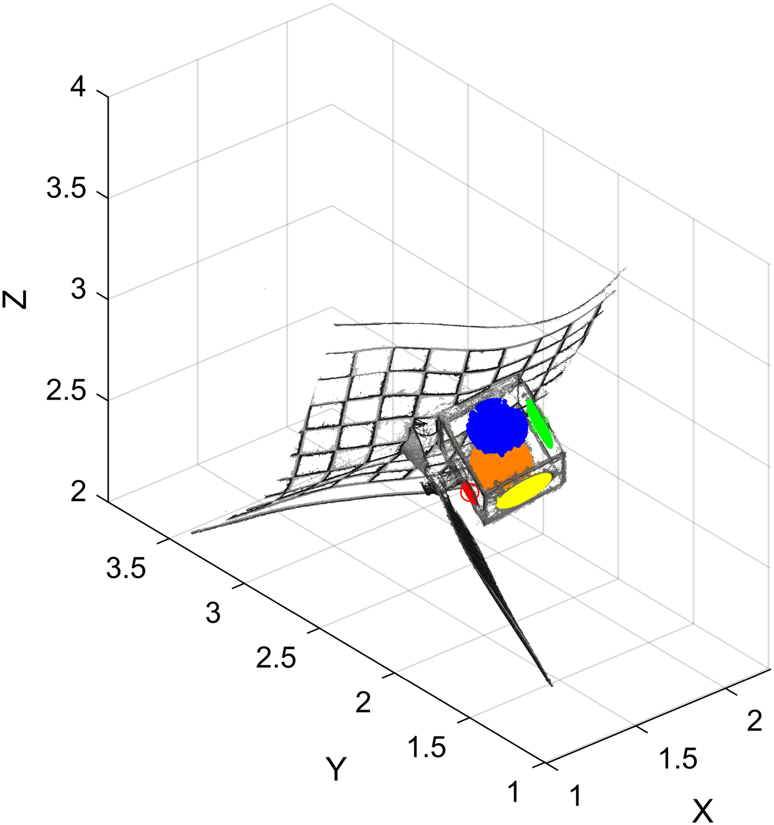
Raw point cloud with points on faces used for alignment highlighted.

A point-to-plane algorithm³⁶ can then be used to match points to their corresponding reference geometry. The algorithm cited was modified to compute the correct scaling. In the work, the rigid transformation is described by a combination of translation and rotation operations described by augmented matrices $T$ and $R$ respectively.

M = T (t_{x}, t_{y}, t_{z}) \cdot R (α, β, γ)

(6)

We add a scaling matrix

S (L)

to the transformation to account for the unknown scale of the point cloud initially.

S (L) = (\begin{matrix} L & 0 & 0 & 0 \\ 0 & L & 0 & 0 \\ 0 & 0 & L & 0 \\ 0 & 0 & 0 & 1 \end{matrix})

(7)

Applying the scaling before the other transformations changes the full transformation to

M = T (t_{x}, t_{y}, t_{z}) \cdot R (α, β, γ) \cdot S (L)

(8)

This propagates well through the subsequent steps in the work, resulting in a slightly altered, but still linear system of equations that can be solved in a similar fashion to the original system.

A x = b

(9)

a = (\begin{matrix} s_{1} \times n_{1} \\ s_{2} \times n_{2} \\ ⋮ \\ s_{N} \times n_{N} \end{matrix})

(10)

A = (\begin{matrix} a_{1 x} a_{1 y} a_{1 z} n_{1 x} n_{1 y} n_{1 z} n s_{1} \\ a_{2 x} a_{2 y} a_{2 z} n_{2 x} n_{2 y} n_{2 z} n s_{2} \\ ⋮ \\ a_{N x} a_{N y} a_{N z} n_{N x} n_{N y} n_{N z} n s_{N} \end{matrix})

(11)

n s_{i} = n_{i x} s_{i x} + n_{i y} s_{i y} + n_{i z} s_{i z}

(12)

x = {(\begin{matrix} α L β L γ L t_{x} t_{y} t_{z} L \end{matrix})}^{T}

(13)

b = (\begin{matrix} n_{1 x} d_{1 x} + n_{1 y} d_{1 y} + n_{1 z} d_{1 z} \\ n_{2 x} d_{2 x} + n_{2 y} d_{2 y} + n_{2 z} d_{2 z} \\ ⋮ \\ n_{N x} d_{N x} + n_{N y} d_{N y} + n_{N z} d_{N z} \end{matrix})

(14)

Here

s_{i} = (s_{i x}, s_{i y}, s_{i z}, 1)^{T}

is a source point,

d_{i} = (d_{i x}, d_{i y}, d_{i z}, 1)^{T}

is the associated destination point, and

n_{i} = (n_{i x}, n_{i y}, n_{i z}, 0)^{T}

is the unit normal vector associated with the destination point.

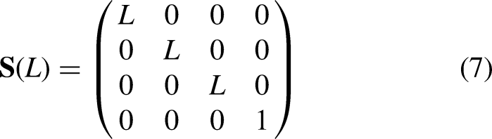
By selecting a minimum of four faces from the reference object, the algorithm is able to align a coordinate system to the object as well as identify a correct scale. Shifting the origin to the desired location on the propeller is then easily done by offsetting the point clouds coordinates using knowledge of the propeller’s mounting to the reference object.

Color based filtering

Since the initial point cloud produced by the photogrammetry is indiscriminate in what objects it digitizes, there are a large number of extraneous data points. We wish to only examine the point cloud representing the propeller blade. Once the point cloud has been transformed into the desired coordinate system, we select a region of interest in the vicinity of the blade and remove all datapoints outside of it. This removes points associated with background objects, leaving just the points associated with the blade to be examined.

An additional challenge is the “noise” present primarily at the leading and trailing edges of the propeller. These points are generally present because the photogrammetry algorithm has no way to distinguish near and far objects at a sharp edge. One option to remove extraneous data is to use a priori knowledge of the propeller color or the background to exclude any points that have an associated color sufficiently close to those of objects we would like to remove. Though relatively simple, the method results in a substantial improvement in the point cloud quality. For this work, a simple euclidean distance was used. If the chosen color to be removed is described by RGB values $r_{filter}$ , $g_{filter}$ , $b_{filter}$ , and the color of the $i$ th point is described by $r_{i}$ , $g_{i}$ , $b_{i}$ , then the criteria to filter certain points out is

\begin{aligned} Remove if \\ (r_{i} - r_{filter})^{2} + (g_{i} - g_{filter})^{2} + (b_{i} - b_{filter})^{2} < c_{filter} \end{aligned}

(15)

The cutoff constant

c_{filter}

requires some tuning to filter the correct points. One method to help identify the cutoff is to plot the distance between the colors on a histogram, such as in Figure 7. If one is seeking to remove a large group of points with similar colors, then there should be a spike near the lower end of the scale. Other dominant colors, like those of the propeller and its pattern, should be grouped together, but have a larger value, suggesting an upper limit for

c_{filter}

Figure 7.

Example histogram showing matches to selected colors within the point cloud with cutoff threshold indicated in red.

Figure 8 illustrates the points removed using such a filtering method and how removing these data points improves the quality of the individual sections. On some parts on the blade, the filtering does remove portions of the blade surface, so care must be taken to ensure that enough data remains for a usable fit.

Figure 8.

Sample of sections along the blade with data filtered out highlighted in red.

Propeller property extraction

Once the point cloud is constructed, there is still the task of converting the raw cloud data into meaningful propeller design parameters. Photogrammetry softwares often have the option to attempt a mesh construction based on the data, but the result is not necessarily superior to working with the point cloud. The mesh is potentially useful in CFD, but does not by itself describe the propeller in a useful parametric format. Figure 9 shows cross sections of an example of a constructed mesh.

Figure 9.

An unscaled automatic triangular mesh produced from the point cloud with cross sections highlighted.

The cross sections show that the generated mesh is not necessarily smooth and that portions of the noisy points on the leading and trailing edge have been incorporated into the geometry. This absorption also removes the points that correctly reflect the position of the leading edge, making identifying its position more difficult. We can instead use the knowledge that the blade was likely designed with a series of airfoils to examine 2D slices of data and fit an airfoil to it to produce geometric information that would be useful for a designer reconstructing the blade. With this approach it is more sensible to use the original point cloud data and fit to all available points rather than do a similar action with a generated mesh.

Propeller design assumptions

We make some basic assumptions of how the propeller is designed - the propeller has relatively smooth functions to describe the chord, twist, and other airfoil properties along the radius. It is also assumed that the propeller is designed using a series of 2D airfoils at various radial stations. This provides a convenient starting point for our geometry extraction. Rather than trying to reconstruct a 3D shape from a point cloud, we can use nearby data to recreate a number of 2D shapes with initial knowledge of what the shape should look like. To be compatible with BET, the geometry is extracted along planes perpendicular to the spanwise axis of the propeller blade. Though this technique may be applied to any airfoil that can be represented by a series of coordinates, this implementation restricts the airfoils to NACA 4-digit series, reducing the optimization space to simply a camber, thickness, and camber location.

Automatic fitting algorithm

In order to minimize required human input, an automatic fitting algorithm was developed to fit 2D contours to the point cloud data. This was done by formulating the problem as an optimization problem to be solved using a coventional optimization software pacakge (e.g., MATLAB’s FMINCON function). This function requires a cost function as well as various constraints. A flowchart illustrating the Automatic Fitting Algorithm is shown in Figure 10.

Figure 10.

Automatic Airfoil Fit Algorithm.

Blade subdivision

To extract the airfoil parameters, a number of radial stations are selected at which to fit the airfoils. At each station, a slice of the point cloud is chosen by defining a plane perpendicular to the Z-axis at this radius and projecting nearby points onto the plane. Increasing the number of points to project allows for more points for fitting the profile, but choosing points that are too far from the section will sample data from an airfoil section that can be significantly different to the airfoil at the the current radius. For the propellers examined in this work, sampling a maximum of 0.25 mm from the plane was found to produce enough points for a reasonable fit while being deemed close enough to accurately represent the chosen 2D section. Once this pseudo 2D data has been assembled, it can then be used to fit a contour.

User input seed

As an initial seed for the rest of the optimizer, a section is chosen at approximately the mid-radius portion of the blade. The user then is presented the section data from a narrow slice in this region and selects the approximate leading and trailing edge locations and the a point in the “up” direction of the profile. To better correspond with typical convention of airfoil coordinates, this selection also defines the coordinate system used for fitting the remaining sections. This coordinate system is defined by an origin at the section leading edge, the airfoil trailing edge being at $[1, 0]$ and the Y-axis pointing in the “up” direction of the airfoil. With this conversion, the airfoil fit should be provided a fairly optimal initial guess. A successful fit can then be used as an initial guess for adjacent sections provided the sections are similar enough to the provided initial guess.

Airfoil fit cost function

In order to determine a best-fit airfoil for the provided data, a cost function is needed. For this work, a distance based least squares function is used, but calculating the distance to an arbitrary contour requires some additional processing. As the contour is represented by a finite series of panels, this is done numerically by calculating the distance to the nearest straight line segment that represents the contour. The result is an optimization statement that can be described by Eq. (16), where $n_{i} (x)$ is the normal distance computed by the $i$ th point based on the contour defined by the parameters $x$ . The problem can also have constraints to $x$ should the user choose, though these would be specific to the parameterization chosen.

\arg min_{x} \sqrt{\sum_{i = 1}^{N} (n_{i} (x))^{2}}

(16)

Panel division

In order to calculate the appropriate panel for a given point, it was necessary to determine which panel represented the “closest” option. To do this, we used angular bisecting domains associated with the interface of each panel to divide the domain into regions of interest. A graphic representation of this is shown in Figure 11. Here, we search for points that best correspond to panel BC. We find this by first looking at its adjacent panels AB and CD. We find the region on the BC side of the bisector to angle ABC, shown in red, and do the same for angle BCD, shown in green. Points in the overlap region are considered to be in panel BC’s region of influence, and their distance from the line segment BC is used to calculate the cost. In high curvature regions, the regions of influence of non-adjacent panels might overlap. In these cases, we examine all the distances to valid panels for a given data point and simply choose the smallest distance to add to the cost.

Figure 11.

Graphical illustration of panel division.

Outlier filtering

Because of the significant amount of noise at the leading and trailing edge of the blade (even with the color-based filtering), it was desired to remove these points from consideration. One approach was to remove approximately the first 5% and last 5% based on chord of the profile data and have the fit carried out on only the mid-section of the data. In cases with substantial amounts of extraneous leading and trailing edge points but good quality midsections, this truncation can improve the fit accuracy.

Chosen parameters

The airfoil at each propeller section is assumed to be sufficiently described by a NACA 4-digit series airfoil⁷ as a wide number of airfoil shapes can be represented through these equations. The equation for describing the thickness of the airfoil is

\begin{aligned} y_{t} & = 5 t [0.2969 \sqrt{x} - 0.1260 x \\ - 0.3516 x^{2} + 0.2843 x^{3} - 0.1015 x^{4}] \end{aligned}

(17)

where

x

is the position from 0 to 1 and

t

is the maximum thickness. The equation to calculate the mean camber line is

y_{c} = {\begin{matrix} \frac{m}{p^{2}} (2 p x - x^{2}), & 0 \leq x \leq p \\ \frac{m}{(1 - p)^{2}} ((1 - 2 p) + 2 p x - x^{2}), & p \leq x \leq 1 \end{matrix}

(18)

where

m

is the maximum camber and

p

is the location of the maximum camber. Lastly, with the adjustment of camber, the ordinates describing the airfoil contour are

x_{U} = x - y_{t} \sin (ϕ), x_{L} = x + y_{t} \sin (ϕ)

(19)

y_{U} = y_{c} + y_{t} \cos (ϕ), y_{L} = y_{c} - y_{t} \cos (ϕ)

(20)

where

ϕ

is defined as

ϕ = \arctan (\frac{d y_{c}}{d x})

(21)

\frac{d y_{c}}{d x} = {\begin{matrix} \frac{2 m}{p^{2}} (p - x), & 0 \leq x \leq p \\ \frac{2 m}{(1 - p)^{2}} (p - x), & p \leq x \leq 1 \end{matrix}

(22)

In addition to the parameters describing the airfoil, we also have the parameters used to fit the airfoil to the point cloud. The parameters used are

Δ x

Δ y

θ

Δ L

. These control the displacement, angle, and scaling from the base airfoil that goes from 0 to 1 on the x-axis to transform it to a position to match the data. The variables are used in the following transformation to transform the airfoil

[\begin{matrix} x_{1} \\ y_{1} \end{matrix}] = Δ L ([\begin{matrix} \cos (θ) & - \sin (θ) \\ \sin (θ) & \cos (θ) \end{matrix}] [\begin{matrix} x_{0} \\ y_{0} \end{matrix}] + [\begin{matrix} Δ x \\ Δ y \end{matrix}])

(23)

Section initial guess and parameter bounds

The user provided input for the initial foil section provides a good initial guess for the airfoil position, meaning that the displacement, angle, and scale should all be close to 0,0, and 1 respectively. The initial airfoil guess is a NACA 0012, but the bounds on the parameters are kept wide as the initial airfoil is not known.

An initial guess is still needed however for each of the remaining sections. A logical choice would be the parameters of an adjacent section. Because we assume the propeller blades studied have continuous geometry, the airfoil properties should also change continuously as we move along the radius. Therefore, for small enough subdivisions, we can use the fit from an adjacent section as an initial guess. Applying parameter bounds that are near this guess allows the airfoil to evolve along the blade while keeping it similar to an adjacent section fit. For the analyses done in this work, the bounds relative to the initial guess were $.1$ chords in each direction for displacement, 3 degrees in each direction for twist angle, and a factor of 20% in either direction for scale.

Optimizer test case

To evaluate the basic functionality of the optimizer, it was run on a pointcloud of artificial data from a known airfoil. The results can be seen in Figure 12 and numerical results are tabulated in Table 2. As is shown, the optimizer produces results accurate to within 10 %, even with introduced positional noise of the data, and with the leading and trailing 10 % of the airfoil truncated to simulate elimination of low quality region from the photogrammetry.

Figure 12.

Demonstration of fitting algorithm results.

Table 2.

Optimizer results on a test case.

Parameter	Thickness (%)	Camber (%)	Cam Loc (%)	dX (l/chord)	dY (l/chord)	$θ$ (deg)	Scale
True	12	2	40	0.1	0.15	2	1.1
Calculated	11.97	1.92	42.04	0.0929	0.1496	1.9766	1.1055
Percent Error	0.23	4.18	$-$ 5.1	7.15	0.24	1.17	$-$ 0.5

Manual extraction

Though the automatic airfoil fitting is convenient, it relies on a priori knowledge of the airfoil type and clean point cloud data. Depending on the availability of these resources, it may be quicker and easier to extract the blade parameters manually using user input. By having the user select the positions of the leading and trailing edges of sampled radial sections, the twist and chord of the blade can be computed in a matter of minutes. This method is useful for some cases such as the APC 10-inch propeller used in this work. As the manufacturer provided an E63 aifoil as the main airfoil used along its span, the airfoil is already known, and extraction of the twist, chord, and leading edge location are the necessary parameters.

Manual extraction can still be used in conjunction with the automatic airfoil fitting. In this case, the optimizer only needs to find optimum values for the airfoil parameters of thickness, camber, and camber location. These values are difficult to extract by hand otherwise, so the automated portions of the process can still provide some utility.

Fitting the airfoils to the cross sections and overlaying them over the processed point cloud can be seen in Figure 13.

Figure 13.

Point Cloud Data with points filtered out in red and fitted airfoils drawn in blue alongside picture of the propeller for reference.

Photogrammetry results

Destructive extraction

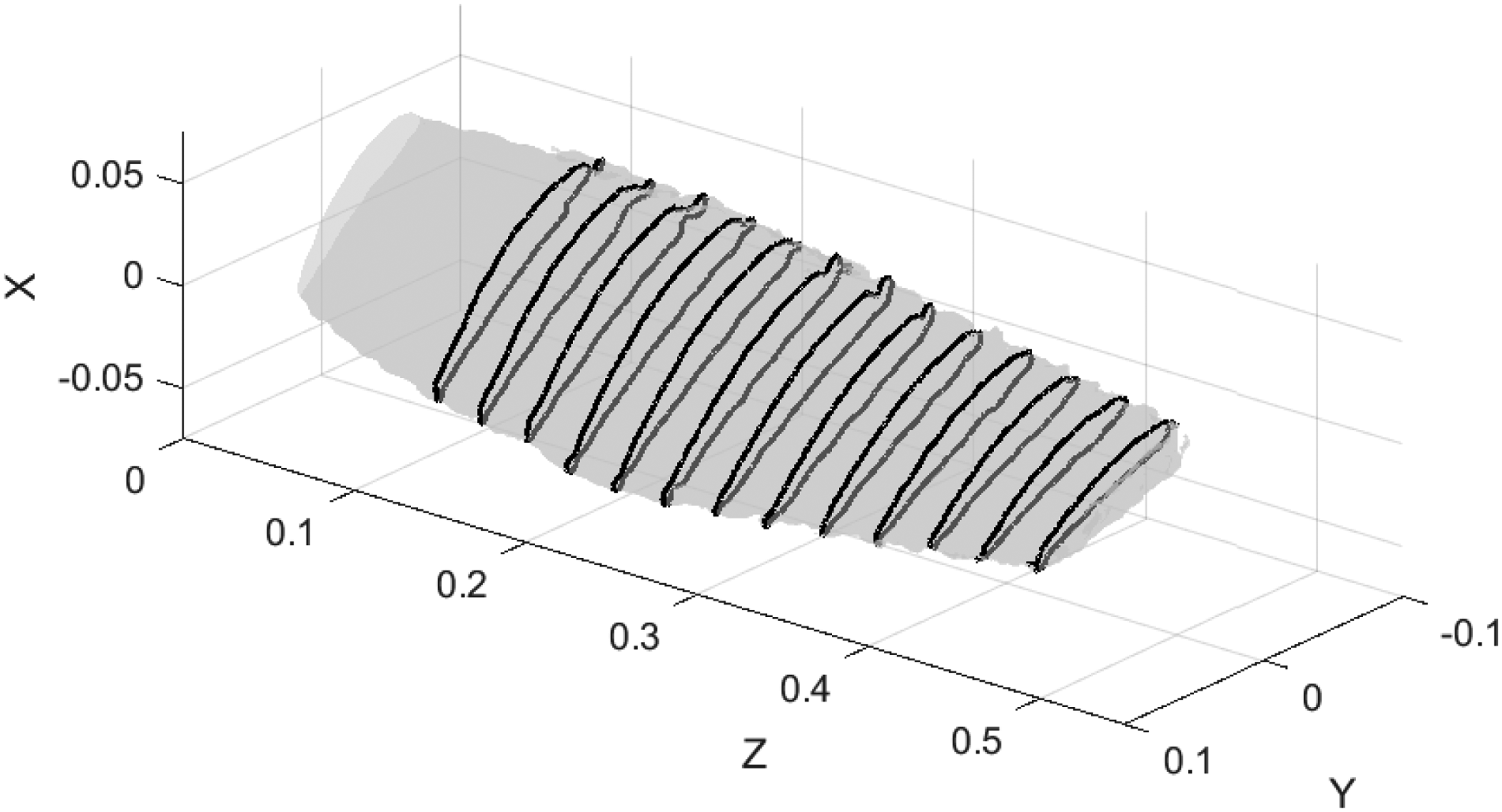
To compare the photogrammetry against some form of truth, the propeller was cast in resin and sliced into sections so that the cross sections could be compared. Casting was done by 3D printing a prismatic mold to place the propeller into and pouring an opaque colored epoxy resin in to fill the void. The enclosure had a mount so that the propeller could be bolted at a known angle relative to the walls of the cast, but some inaccuracy in this persisted, as described later. Once the epoxy set, it was removed from the mold and sliced into wafers on a vertical milling machine using a slitting saw. 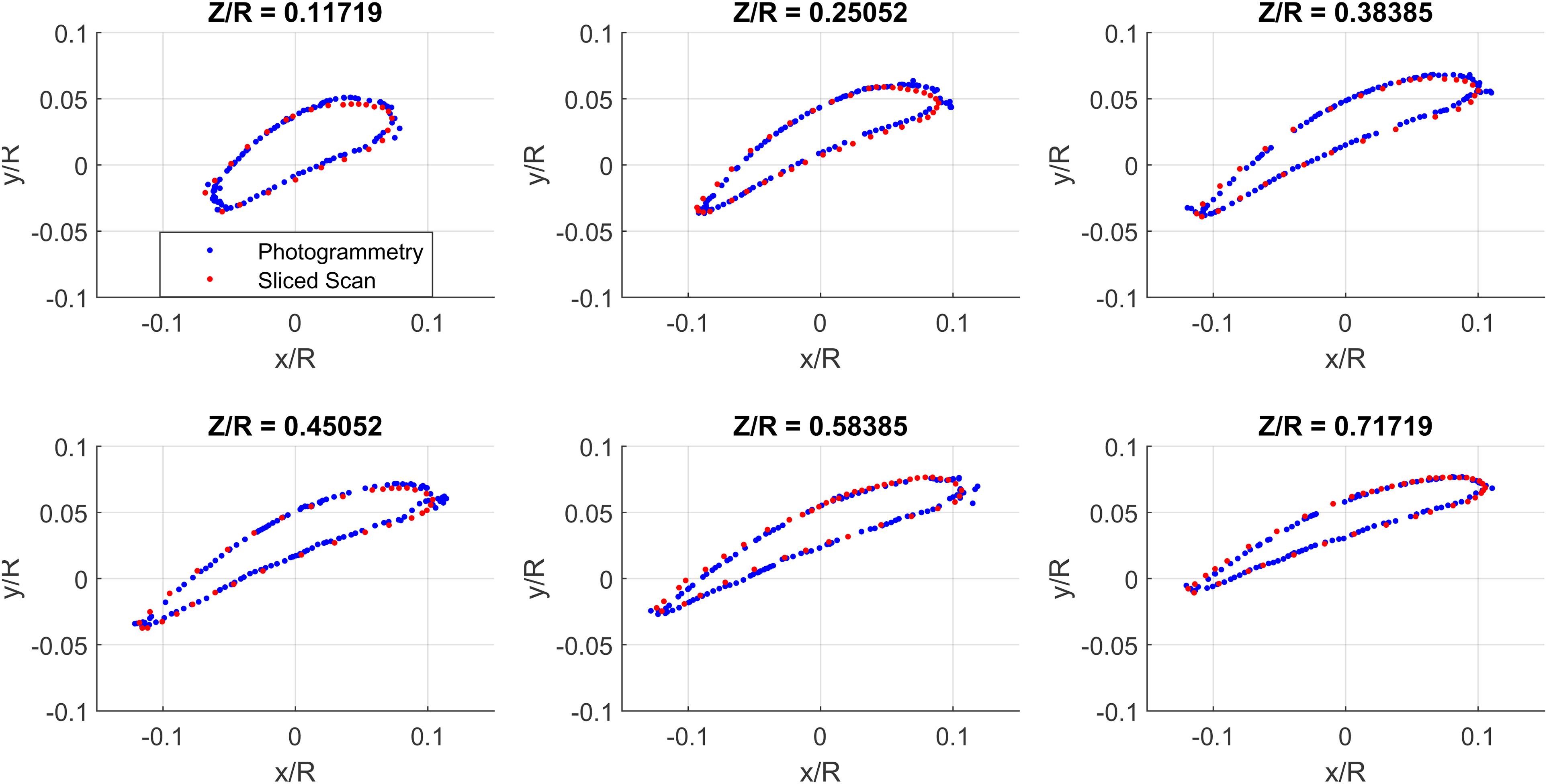By using the vertical mill’s digital encoders, the relative position of the faces of each of the sliced wafers was known to high accuracy ( $\approx$ 0.025 mm). Each wafer was then scanned on an Epson V600 scanner at 6400 dpi to digitize each section. The section contours were found using a subpixel edge detection algorithm.³⁷ Figure 14 shows that the curves at arbitrary stations produced by photogrammetry show close agreement with the points collected during the destructive extraction.

Figure 14.

Comparison between point cloud and sliced section data on the DALPROP 6045.

Photogrammetry resolution

The algorithm used by COLMAP relies on the presence of “corners” within the image, something a grid provides. Nevertheless, some loss of accuracy can still be seen within regions of one color. For example, as seen in Figure 15a, the points in the regions between the black lines appear to have a larger spread than in the regions at the color interfaces.

Figure 15.

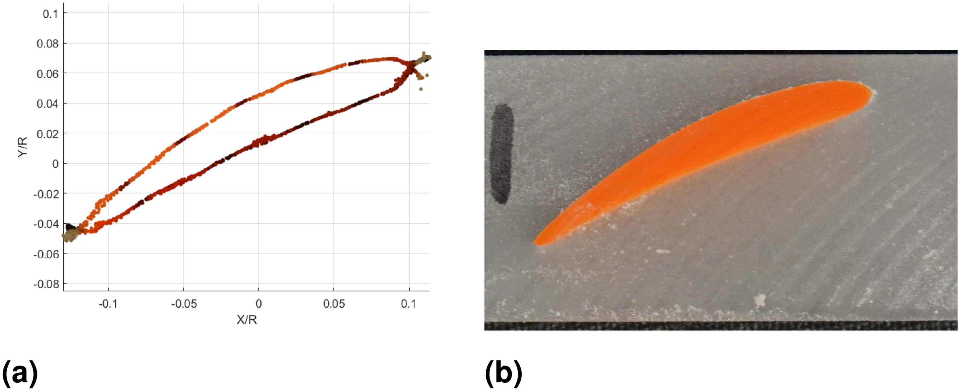
Illustration of accuracy of point cloud versus the physical section.

Note that the physical section seen in Figure 15b which is the same station as the points sample for Figure 15a does not converge to a point at the trailing edge as one might expect an airfoil, but that the photogrammetry still qualitatively picks up the slightly blunt trailing edge.

Determining a metric for error in the process is difficult because of a lack of a geometric truth for the propellers evaluated. Even the destructive extraction requires optical measurement and still only produces points rather than a contour against which to check accuracy. As a measure of the point cloud accuracy, we compute the root mean square of the normal distance from the airfoil contour that is fit at each section of the point cloud to each of the points used for that section. The results for the 5 propellers scanned in this work are shown in Figures 16 and 17.

Figure 16.

RMSE position error relative to fitted airfoil along propeller radius.

Figure 17.

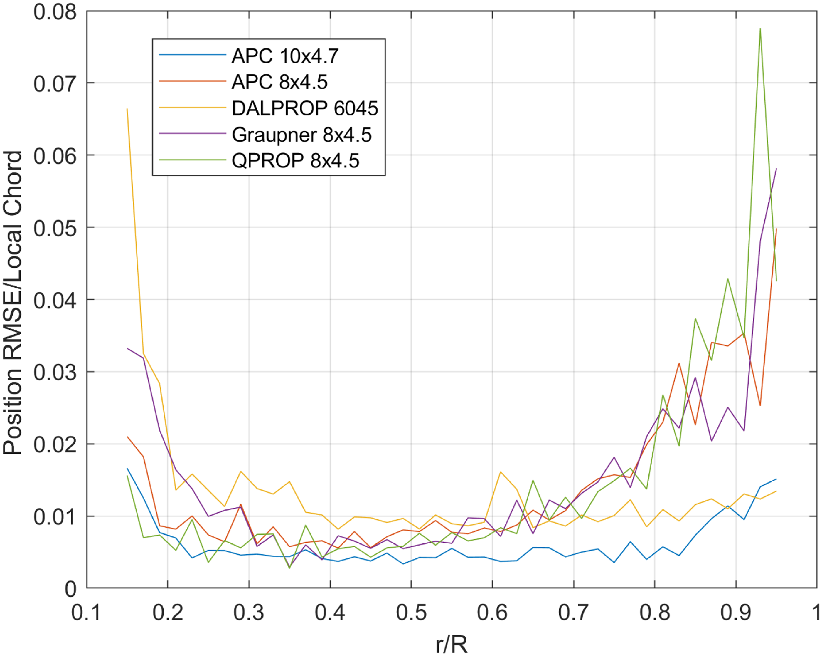
RMSE position error relative to fitted airfoil along propeller radius, normalized by local chord.

We see that, relative to the fit airfoil, positional error varies significantly by radial position. Figure 16 shows that the estimated error is comparable to the desired level of accuracy of 0.1 mm for much of the blade. At the blade root, the higher error is expected, as the profiles here begin to blend into the propeller hub, and do not correspond well to the NACA 4-digit series. Near the tip, the error is again high as expected. The photogrammetry algorithm has difficulty with edges, leading to a larger number of extraneous points as well as points associated with the background, that are falsely attributed to the blade. The 10 inch APC and the Dalprop propellers have relatively low error in the tip region, likely because their colors (grey and orange respectively) have high contrast relative to the background and extraneous points are more easily filtered out. The remaining propellers are all black with a white pattern drawn on, which ended up not being sufficiently high contrast to the background. The fact that the chord tends to decrease near the propeller tip also accentuates the apparent error, visible by comparing the tip regions of Fig. Figures 16 and 17. In regions with good quality, such as in the vicinity of 0.5 r/R, the error for all the propellers is less that 1%, which is within the goal specified above to be able to differentiate different airfoils within the NACA 4-digit family. This corresponds to a dimensional accuracy of roughly 0.15 mm in most instances on these propellers.

Comparison of parameters

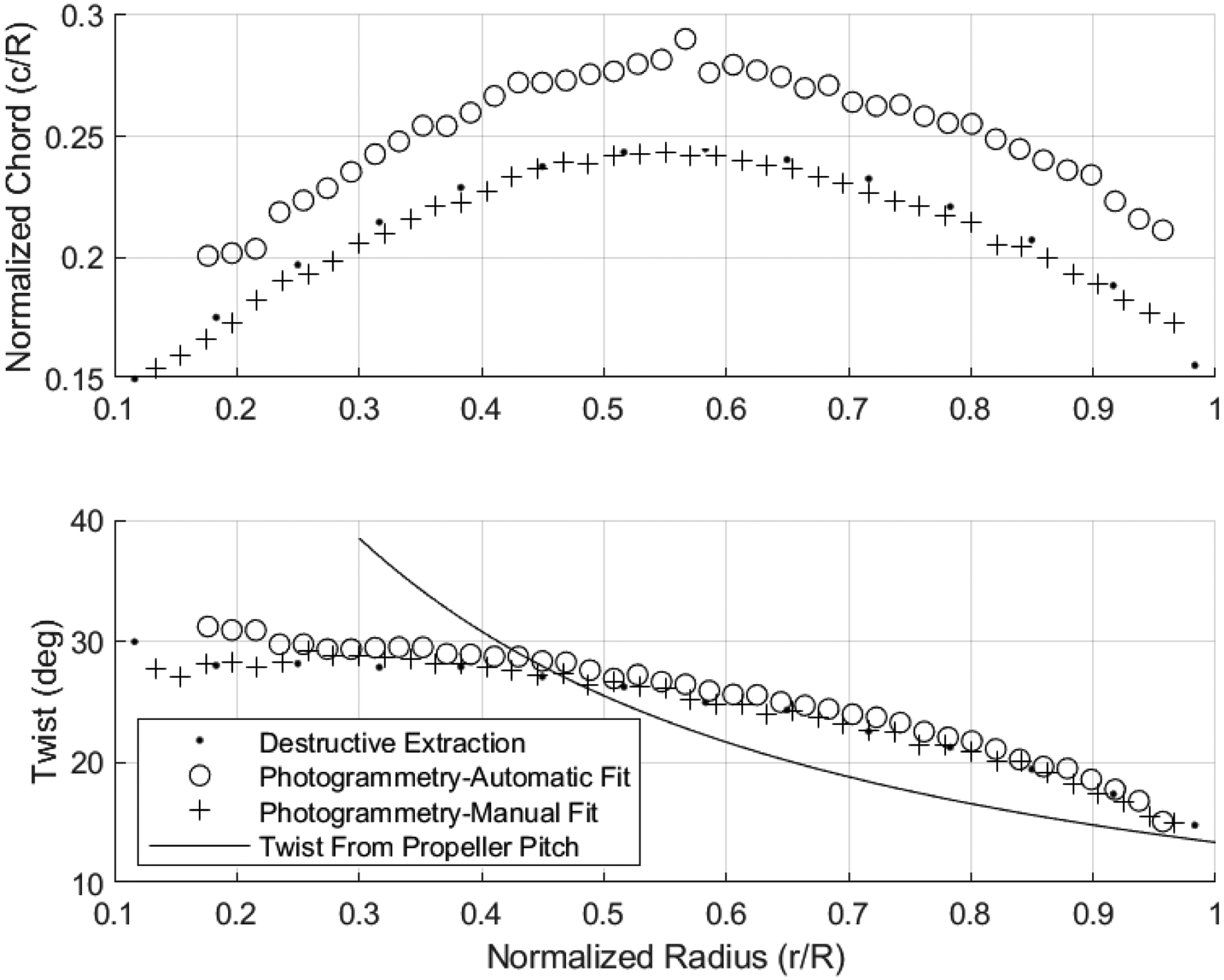
For the 10-inch APC propeller, we can compare basic propeller metrics between the published values, the destructive extraction, and the photogrammetry. In Figure 18, we see that the contours of the published data, the destructive extraction, and the photogrammetry are in close agreement. In fact, the destructive extraction technique appears to have a fixed offset error in the twist angle. This is likely caused by either a consistent error in how the cut sections were positioned in the scanner, or an error in the propeller angle in the casting prior to slicing. The error it highlights the difficulty of correctly aligning the propeller when analyzing its sections, as even a few degrees of misalignment will translate to the extracted specifications. Also plotted on the twist graph is the twist angle computed by the advertised blade pitch, which shows that APC’s propeller follows the contour quite closely.

Figure 18.

Comparison of Twist and Chord extracted using various methods for a 10-inch propeller.

Figure 19 shows a similar analysis for the 6-inch propeller, and also demonstrates the accuracy of the automatic fit. While the automatic fit has good agreement with the shape of each curve, it is offset slightly in chord magnitude. The cause of this can be traced to the chosen airfoil type used for fitting. As shown in Figure 20, although the airfoil fit matches the upper and lower surfaces of the airfoil on the 6-inch prop well, the truncated section leads to the fit overestimating the chord and, due to the camber, dropping the trailing edge leading to an overestimation of the local twist. If a airfoil with a different parameters that was capable of matching the true shape better were used in the fitting algorithm, the twist and chord would likely be more accurate. Again, the twist computed using the propeller pitch is plotted as well. Unlike the APC prop, this propeller seems to use the pitch length as more of a mild suggestion. The fact that this propeller does not use the pitch length as the basis for its twist distribution highlights the importance of extracting the geometry rather than relying on assumptions of the propeller design.

Figure 19.

Comparison of Twist and Chord extracted using various methods for a 6-inch propeller.

Figure 20.

Fitted airfoil to section from 6-inch propeller.

Extraction of airfoil camber and thickness is tedious, even with high quality points representing the upper and lower surfaces. This is because the points are unstructured, while computing camber and thickness requires comparing coordinates for points that are at the same station along the chord. Nevertheless, a best attempt at calculating these values is illustrated for the 6 inch propeller in Figure 21. As is expected, there is a fair amount of noise in these measurements along the span, and they have similar shapes but some disagreement. The difference in thickness can be explained as before by the fitting producing a longer chord than the true section. A longer chord for the same thickness would produce a lower thickness ratio than truth.

Figure 21.

Comparison of Camber and Thickness extracted using various methods for a 6-inch propeller.

Propeller force prediction

Experimental data

Force and torque data were collected for the propellers studied on a commercial off the shelf RC Benchmark 1585 thrust stand. The stand takes real time measurements of thrust, torque, current, and other relevant performance data. The stand also features a scripting mode which allows it to spin the propeller in a sweep of rotational speeds and record the data automatically. Once the data are collected, they can be compared to the experimental data at similar operating conditions.

Simulation prediction

With the geometry of the propeller known, the propeller can be modeled and simulated for a variety of analyses. To simulate the performance of each of the propellers scanned, we use the software QPROP.³⁸ QPROP uses a classical blade element and vortex formulation described in its associated theory guide.

One requirement of BET is to have some model of the section lift and drag for sections along the propeller blade. Determining the lift and drag polars for an arbitrary airfoil section is done numerically as there is no guarantee that the fitted section corresponds to one with available data. The airfoil performance is calculated using XFOIL,³⁹ and the subsequent information provided to QPROP. QPROP models the airfoil properties in the following manner

c_{l} (α) = (C_{L_{0}} + C_{L_{a}} α) \frac{1}{\sqrt{1 - M^{2}}}

(24)

where

C_{L_{0}}

is the lift coefficient at 0 angle of attack,

C_{L_{a}}

is the lift curve slope, and

M

is the Mach number, which is used for the local Prantdl-Meyer compressibility factor. The bounds of the airfoil model are also specified with the variables

C_{L_{m i n}}

and

C_{L_{m a x}}

indicating the minimum and maximum lift coefficients. The drag coefficient of the airfoil is modeled as

c_{d} (c_{l}, R e) = [C_{D_{0}} + C_{D_{2}} (c_{l} - C_{L} C_{D 0})^{2}] [R e / R e_{ref}]^{R e_{\exp}}

(25)

where

C_{D_{2}} = C_{D_{2} u} if c_{l} > C_{L} C_{D 0}

(26)

C_{D_{2}} = C_{D_{2} l} if c_{l} < C_{L} C_{D 0}

(27)

The drag model for the airfoil features a Reynolds number correction.

R e_{ref}

is the Reynolds number at which the other airfoil properties are referenced, while

R e

is the section Reynolds number.

R e_{\exp}

is a constant that can be adjusted based on the flow conditions. The program does not feature such an adjustment for the lift curve. Analysis in XFOIL indicates that the

C_{L_{0}}

computed for some of the fitted airfoils changes significantly based upon the Reynolds number within the expected range of Reynolds numbers for these propellers. The lack of correction could be a source of error in the analysis. Additionally, the local chord based Reynolds numbers along the blade for most of the propellers in this work are in the range of 1 000s to 150 000, meaning that the Reynolds number is often low enough for the accuracy of XFOIL to be uncertain. To help mitigate the effect of the change in properties with Reynolds number, Reynolds number specific airfoil properties are defined at each station along the blade span for the simulation.

The comparison of experimental results to the predicted performance presented in Figure 22 shows good agreement in thrust for the propellers studied. We also examine the agreement between the Thrust and Torque coefficients, defined as $T = ρ ω^{2} C_{T} D^{4}$ and $Q = ρ ω^{2} C_{Q} D^{5}$ respectively. Here, $ρ$ is the air density, $ω$ is the rotation speed of the propeller in $r a d / s$ , and $D$ is the propeller diameter. Predicted and measured coefficients for each propeller are seen in Figure 23a and b. Predicted thrust coefficients are within 10% of the measured value for the propellers, however torque predictions feature much greater error. This is likely due to the inherent difficulty of accurately predicting drag at lower Reynolds numbers. In particular, the DALPROP 6045 featured a larger mismatch in torque than the other propellers. One possible reason for this mismatch is that the airfoil section for this propeller has a blunt trailing edge, further increasing the difficulty of accurate drag prediction. The simulation results were found to be highly sensitive to a variety of different parameters. Applying a blade pitch of even a few degrees significantly changed the thrust results. One example of this is found by comparing the HQProp and the APC 8-inch propeller. Though sold by different entities, these propellers happen to be nearly exactly the same in terms of visual inspection. The photogrammetry results confirm this, with the data indicating they possess nearly identical chord, thickness, and camber distribution. The main difference is in the twist distribution, where both propellers have nearly identical contours, but the HQProp has 2 degrees of difference in pitch across the blade. This difference is evident in the experimental thrust data where the APC propeller has a 17% higher thrust coefficient than the HQProp propeller.

Figure 22.

Comparison of experimental results of propeller to simulation in QPROP.

Figure 23.

Comparison of Non-Dimensional Coefficients from Simulation and Experiment.

Conclusion

While many forms of 3D scanning technologies exist, they are often costly or inaccessible to many researchers. This paper has developed a technique that shows that with freely available software, commonly available computing hardware, and today’s high-resolution cameras, photogrammetry with accuracy sufficient for BEM can be achieved with little expertise or dedicated equipment. The point clouds produced by photogrammetry are accurate enough to extract the propeller geometric parameters at a resolution comparable to competing 3D scanning methods. The use of the point-to-plane algorithm for automated orientation as well as the airfoil fitting methods allow for rapid extraction of useful propeller parameters rather than just an unstructured mesh or point cloud, thereby facilitating the import of the model into a parametric design software.

Subsequent simulation of the extracted geometry shows good agreement with experimental results in thrust. As accurate geometry is a critical requirement of performing credible simulations, the authors expect that the technique developed will benefit the aerospace research community. The implementation of this work can be found at https://github.com/ellandetang/PhotoFoil

Footnotes

Acknowledgments

The authors thank Matt Anderson for his constructive feedback and guidance.

Declaration of conflicting interests

The authors declared no potential conflicts of interest with respect to the research, authorship, and/or publication of this article.

Funding

This work was supported using a National Defense Science and Engineering Graduate (NDSEG) fellowship administered via the Air Force Office of Scientific Research.

ORCID iD

Ellande Tang

References

Leishman

. Blade Element Analysis. In Principles of Helicopter Aerodynamics, 2 ed, chapter 3. Cambridge University Press. ISBN 9781107013353, 2016. pp. 115–158.

Leishman

. Momentum Theory Analysis in Hovering Flight. In Principles of Helicopter Aerodynamics, 2 ed, chapter 2.2. Cambridge University Press. ISBN 9781107013353, 2016. pp. 58–64.

Alvarez

Ning

. High-fidelity modeling of multirotor aerodynamic interactions for aircraft design. AIAA J 2020; 58: 4385–4400.

Yoon

Lee

Pulliam

. Computational Analysis of Multi-Rotor Flows. In 54th AIAA Aerospace Sciences Meeting. Reston, Virginia: American Institute of Aeronautics and Astronautics. ISBN 978-1-62410-393-3. doi:10.2514/6.2016-0812. https://arc.aiaa.org/doi/10.2514/6.2016-0812.

APC. APC Technical Information - Engineering - Airfoils, 2021. https://www.apcprop.com/technical-information/engineering/#ai.

Brandt

Deters

Ananda

et al. UIUC Propeller Database, Vols 1-3, 2020. https://m-selig.ae.illinois.edu/props/propDB.html.

Abbott

von Doenhoff

. Theory of Wing Sections: Including a Summary of Airfoil Data. Dover Publications, 1959. ISBN 9780486605869.

Chapman

ed. Handbook for the metalworking industries. 1st ed. Cincinnati, OH: Gardner Publications, 2002.

Hexagon. Coordinate Measuring Machine Accuracy on the Shop Floor, 2022. https://www.hexagonmi.com/solutions/technical-resources/techn.

10.

Menna

Troisi

. Low cost reverse engineering techniques for 3D modelling of propellers. Int Arch Photogramm, Remote Sens Spat Inform Sci - ISPRS Arch 2010; 38: 452–457.

11.

MSC. 117mm Long CMM Motorized Probe Head, 2022. https://www.mscdirect.com/browse/tnpla/31241045.

12.

Shaheen

Mohammed

. Reverse engineering using laser scanned and manufacturing of A powered paraglider propeller. J Multidiscip Eng Sci Technol (JMEST) 2020; 7: 12810–12815.

13.

Prudden

. Rotor Aerodynamic Interaction Effects for Multirotor Unmanned Aircraft Systems in Forward Flight. PhD Thesis, RMIT University, 2020.

14.

Chua

. Simulating the effect of non-axial airflow on the motion of an undriven propeller. Int J Adv Trends Comput Sci Eng 2020; 9: 153–159.

15.

Drela

. Propeller Characterization for QPROP, 2005. http://web.mit.edu/drela/Public/web/qprop/prop_measure.pdf.

16.

Gary Hinze. Propeller Gauges, 2016. http://www.endlesslift.com/propeller-gauges/.

17.

Luhmann

. Close range photogrammetry for industrial applications. ISPRS J Photogramm Remote Sens 2010; 65: 558–569.

18.

Liu

Cattafesta

Radeztsky

et al. Photogrammetry applied to wind-tunnel testing. AIAA J 2000; 38: 964–971.

19.

Jennings

Black

. Texture-based photogrammetry accuracy on curved surfaces. AIAA J 2012; 50: 1060–1071.

20.

Setan

Ibrahim

. Digital Close Range Photogrammetric System For High Precision Propeller Measurement. In Malaysian Science & Technology Congress. January.

21.

PhotoModeler Scanner, 2022. https://www.photomodeler.com/products/scanner/.

22.

Vergauwen

Van Gool

. Web-based 3D reconstruction service. Mach Vis Appl 2006; 17: 411–426.

23.

Ackermann

Menna

Scamardella

et al. Digital photogrammetry for high precision 3D measurements in shipbuilding field. 6th CIRP Int Conf on ICME 2008; 1(January): 6–11.

24.

Amini

Varshosaz

Saadatseresht

. Deformation determination of aircraft parts by photogrammetry. Int Arch Photogramm, Remote Sens Spat Inform Sci - ISPRS Arch 2008; 37: 135–138.

25.

Tang

Chung

. Rapid extraction of propeller geometry using photogrammetry. Bull Am Phys Soc 2021; 66. https://meetings.aps.org/Meeting/DFD21/Session/E20.1.

26.

Schönberger

Zheng

Pollefeys

et al. Pixelwise View Selection for Unstructured Multi-View Stereo. In European Conference on Computer Vision (ECCV).

27.

Schönberger

Frahm

. Structure-from-Motion Revisited. In Conference on Computer Vision and Pattern Recognition (CVPR).

28.

Griwodz

Gasparini

Calvet

et al. AliceVision Meshroom: An open-source 3D reconstruction pipeline. In Proceedings of the 12th ACM Multimedia Systems Conference. ACM Press. doi:10.1145/3458305.3478443.

29.

Rupnik

Daakir

Pierrot Deseilligny

. MicMac – a free, open-source solution for photogrammetry. Open Geospatial Data, Software Stand 2017; 2: 14.

30.

Fuhrmann

Langguth

Moehrle

et al. MVE—an image-based reconstruction environment. Comput Graph 2015; 53: 44–53.

31.

Moulon

Monasse

Perrot

et al. OpenMVG: Open multiple view geometry. In International Workshop on Reproducible Research in Pattern Recognition. Springer, pp. 60–74. doi:10.1007/978-3-319-56414-2_5.

32.

Rahaman

. Regard3D, 2022. http://www.regard3d.org/index.php.

33.

. VisualSFM: A Visual Structure from Motion System, 2011. http://ccwu.me/vsfm/.

34.

Agarwal

Curless

et al. Multicore Bundle Adjustment. In Computer Vision and Pattern Recognition.

35.

. Towards Linear-Time Incremental Structure from Motion. In 2013 International Conference on 3D Vision - 3DV 2013. IEEE. ISBN 9780769550671, pp. 127–134. doi:10.1109/3DV.2013.25.

36.

Low

. Linear Least-squares Optimization for Point-to-plane ICP Surface Registration. Chapel Hill, University of North Carolina 2004; https://www.iscs.nus.edu.sg/lowkl/publications/lowk_poi.

37.

Trujillo-Pino

. Accurate subpixel edge location, 2021. https://www.mathworks.com/matlabcentral/fileexchange/48908-ac.

38.

Drela

. QPROP-Propeller/Windmill Analysis and Design, 2007. http://web.mit.edu/drela/Public/web/qprop/.

39.

Drela

Youngren

. XFOIL-Subsonic Airfoil Development Sytem, 2013. https://web.mit.edu/drela/Public/web/xfoil/.