Sage Journals: Discover world-class research

Abstract

Recently, the concept of incremental nonlinear dynamic inversion has seen an increasing adoption as an attitude control method for a variety of aircraft configurations. The reasons for this are good stability and robustness properties, moderate computation requirements and low requirements on modelling fidelity. While previous work investigated the robust stability properties of incremental nonlinear dynamic inversion, the actual closed-loop performance may degrade severely in the face of model uncertainty. We address this issue by first analysing the effects of modelling errors on the closed-loop performance by observing the movement of the system poles. Based on this, we analyse the neccessary modelling fidelity and propose simple modelling methods for the usual actuators found on small-scale electric aircraft. Finally, we analyse the actuator models using (flight) test data where possible.

Keywords

Attitude control tiltwing incremental nonlinear dynamic inversion

Introduction

Incremental nonlinear dynamic inversion (INDI) has been applied to a variety of aircraft including quadrotors, hybrid aircraft (tailsitter, tiltwing) and conventional airplanes.^1–4 In comparison to classical control techniques, its benefits lie in the achievable level of robustness and performance, the ease of controller tuning and the economical implementation aspects. 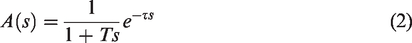The method was first introduced by NASA⁵ and then further developed at TU Delft.^1,2 At the core of INDI, a simple control law given by

δ u = M_{u}^{- 1} \cdot J \cdot (ν - \dot{Ω})

(1)

is used, where ν is the commanded angular acceleration, J is the aircrafts inertia and

M_{u}

describes the actuator effectivity. This paper concentrates on the last term

M_{u}

and the associated neccessary dynamic actuator models. We summarise modelling approaches which have been successfully applied in practice for quadrotors,² tiltwing⁶ or tailsitter^3,7 aircraft. Since the problem of oscillations frequently arises when applying INDI, we try to gain some insight into this issue by observing the closed-loop system poles. A similar analysis was already done in previous work⁸ but concentrates on the stability properties of the closed loop.

Effects of modelling uncertainty

The goal of nonlinear dynamic inversion (NDI) is to invert the plant dynamics so that the resulting closed-loop dynamics are a series of integrators. In principle, the INDI formulation in Smeur et al.² shares this goal. However, due to the way in which state-derivatives (i. e. angular accelerations) are calculated, the resulting closed-loop dynamics from the commanded angular accelerations ν to the actual angular accelerations $\dot{Ω}$ are the actuator dynamics A(z) in the nominal case. Thus, the design of outer controllers (e.g. angular rate and attitude controllers) is influenced by these actuator dynamics A(z). One major motivation in using NDI (or INDI) is to simplify the design of outer loop controllers. We thus want to develop an understanding of how well the actuator dynamics and effectivity needs to be known, to still achieve an appropriate outer loop performance.

To analyse this, we assume an INDI-based angular rate controller, as shown in Figure 1. For simplicity, we only analyse the single-input single-output case but expect the results to be transferable in principle to the multiple-input multiple-output case as well. The parameters of the system consist of the plant parameters – namely, the control effectivity $M_{η}$ , actuator time constant T and actuator delay τ – and the corresponding controller parameters ${\hat{M}}_{u}, \hat{T}, \hat{τ}$ . The actuator dynamics are modelled as first-order lags with an optional delay

A (s) = \frac{1}{1 + T s} e^{- τ s}

(2)

Figure 1.

Controller structure.

In the nominal case, ${\hat{M}}_{u} = M_{u}, \hat{T} = T$ and $\hat{τ} = τ$ . To develop an understanding of how uncertainty in the parameters affects the closed-loop system, we analyse movement of the system poles when parameters are changed.

Poles of the INDI controller

In the nominal case, the closed-loop transfer function from the commanded angular accelerations ν to the actual angular accelerations $\dot{Ω}$ is equal to the actuator dynamics A. In the non-nominal case, additional dynamics appear because the system poles and zeros do not cancel each other. Since the analytical expression for the closed-loop transfer function in the non-nominal case is somewhat convoluted, we graphically analyse the behaviour of the poles instead. While INDI is an inherently discrete-time control algorithm, we choose to display the poles (and zeros) in the continuous-time domain because we are more familiar with this setting.

Figure 2 shows the movement of the poles of the INDI loop, when the control effectivity M_u is incorrect. In the nominal case (left), the poles of the filter H are completely cancelled and thus do not influence the closed-loop dynamics. Only the poles of the actuator dynamics A remain. We selected the filter parameters of H as follows

\begin{array}{l} H (s) = \frac{ω_{0}^{2}}{s^{2} + 2 ζ ω_{0} s + ω_{0}^{2}} \\ ω_{0} = 50 {rads}^{- 1} \\ ζ = 0.55 \end{array}

(3)

Figure 2.

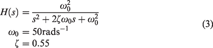
Effect of uncertainty in control effectivity on significant poles of INDI loop, $0.2 < {\hat{M}}_{u} / M_{u} < 4$ .

For ${\hat{M}}_{u} \neq M_{u}$ , the cancellation of the filter poles does not occur. For ${\hat{M}}_{u} < M_{u}$ , the poles of the filter H become less damped and start to show as oscillations in the time domain. The frequency of this oscillation roughly equals the natural frequency ω₀ of the filter H. For ${\hat{M}}_{u} > M_{u}$ , the system dynamics basically slows down because the poles of the assumed actuator dynamics $\hat{A}$ move to the right. For the chosen filter parameters (see equation (3)), the closed loop becomes unstable for $\frac{{\hat{M}}_{u}}{M_{u}} < 0.2$ , though clearly visible oscillations start to appear at around $\frac{{\hat{M}}_{u}}{M_{u}} < 0.5$ . Note that these margins change when choosing different filter parameters H. In general, a larger damping ratio ζ and a larger natural frequency ω₀ lead to more robustness w.r.t. uncertainty in M_u. At the same time, these filter parameters influence the amount of noise introduced when calculating $\dot{Ω}$ as well as the disturbance rejection performance.² Thus, the filter parameters will be a trade-off between robustness w.r.t. to M_u, performance of disturbance rejection and noise. The exact nature of this trade-off is part of future work and not yet explored further.

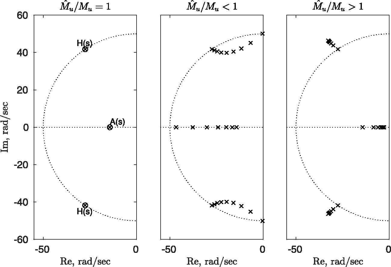
Figure 3 shows a similar analysis as before, this time changing the assumed actuator dynamics $\hat{T}$ . Here, for $\hat{T} < T$ , the poles associated with the actuator dynamics become underdamped and move towards lower damping while the frequency stays roughly the same. Again, the more benign direction is an overestimation of the actuator time constant $\hat{T}$ , since in this case the most significant pole merely moves towards lower frequencies while still being fully damped.

Figure 3.

Effect of uncertainty in actuator dynamics on significant poles of INDI loop, $T = 0.07, 0.01 < \hat{T} < 0.14$ .

Finally, Figure 4 shows a similar analysis for the effect of uncertainty in the time delay $\hat{τ}$ . As was already discussed in the literature,⁸ a lack of assumed time delay $\hat{τ}$ can lead to oscillations in the closed loop. In case of underestimating the delay $\hat{τ}$ , the significant poles first tend towards faster dynamics while still being fully damped. Once a critical error in the estimated delay $\hat{τ}$ is reached, the dynamics become underdamped. The more benign case is again an overestimation of the delay $\hat{τ}$ , which leads to slower system dynamics. However, with an increasing overestimation of $\hat{τ}$ , the poles of the filter H become less damped and lead to visible oscillations in the time-domain response. Unfortunately, an error in the estimated delay leads to a behaviour, which is similar to the behaviour in case of an error in either the control effectivity M_u or the actuator time constant T. Determination of the delay τ can, however, be quite easily accomplished by either analysing flight test data or performing dedicated testing of the actuators.

Figure 4.

Effect of uncertainty in actuator delay on significant poles of INDI loop (sample time $T_{s} = 0.001 sec$ ), $τ / T_{s} = 40, 0 < \hat{τ} / T_{s} < 80$ .

In summary, this analysis gives some insight into the behaviour of INDI in case of uncertainty. In our experience, a common problem when implementing INDI for a new aircraft are oscillations. Based on the discussion above, observing the frequency of the oscillations can give a hint as to what the source of the oscillations is. Appropriate mitigations can either be to adapt the assumed model ( ${\hat{M}}_{u}, \hat{T}, \hat{τ}$ ) accordingly or the parameters ( $ω_{0}, ζ$ ) of the filter H. Additionally, overestimation of the control effectivity M_u and the actuator time constant T generally leads to slower dynamics and thus might serve as a good starting point for new controller designs. In ‘Analysis’ section, we show how the performance of an INDI controller can easily be assessed and tuned in real-time, enabling rapid controller development.

Actuator models

Small electric aircraft typically features two kinds of actuators: rudders and electric motors with propellers to produce thrust. Depending on the configuration, the rudders might additionally be positioned in the slip-stream of the propellers. This configuration is often used to create rudder effectivity even when there is no aerodynamic velocity (e.g. flying-wings, tiltwing aircraft).

To model the effectivity of these actuators, we propose a two-step approach: First, we calculate the thrust, slip-stream velocity and effectivity of the motors. Second, we calculate the effectivity of the rudders, taking into acount slip-stream velocities if neccessary.

In addition to these static actuator model properties, we also model the dynamic behaviour of the actuators. This is of course only strictly necessary, when the actuator positions are not measured. Still, for designing the outer rate and attitude controllers, an estimate of the actuator dynamics is beneficial.

For both the static and dynamic properties, we rely as much as possible on properties which are either easily measurable or specified by the manufacturers. In ‘Analysis’ section, we analyse how well these actuator models actually perform and how this compares to the requirements on modelling fidelity derived in ‘Effects of modelling uncertainty’ section.

Static actuator effectivity models

Within the scope of attitude control, the actuator effectivity describes the change in moments due to changes in actuator position (i.e. rudder deflection or throttle). For many applications, it is sufficient to look at the force induced by an actuator and use the corresponding lever to calculate the induced moment. We thus get expressions of the form

M_{u} = \frac{\partial M}{\partial u} = r \times \frac{\partial F}{\partial u}

(4)

where

M_{u}

describes the actuator effectivity of an actuator u in the body-fixed coordinate frame given by the cross-product of the actuator position r and the induced change in force F. In the following section, we will mostly focus on determining the term

\partial F / \partial u

Motors

The most common type of electric motor used in electric aircraft is the synchronous AC motor. It needs to be driven by a specialised electronic component called an electronic speed controller (ESC), see Figure 5. An ESC is controlled via a throttle value δ, which can typically be normalised to ranges from 0 to 1 (or −1 to 1, if the ESC supports driving the motor in reverse). The ESC generates the appropriate voltages to drive the motor, resulting in an angular velocity measured as revolutions per minute (RPM) n. Depending on the propeller and inflow conditions, these angular velocities then result in a thrust F. This description makes the simplifying assumption that the angular velocity is independent of the inflow. It thus enables using a simpler model at the cost of modelling fidelity.

Figure 5.

Motor model. ESC: electronic speed controller; BLDC: Brushless Direct-Current Electric Motor .

The motor model we propose consists of two parts: a mapping from the throttle δ and the supply voltage U of the ESC to the RPM n and a mapping from n combined with the inflow V_a to the thrust F.

ESC/Brushless Direct-Current Electric Motor (BLDC) model

When the motor RPM are not measured, we use the following model based on the supply voltage U, the motor speed constant K_V and the throttle setting δ

n = U \cdot K_{V} \cdot δ

(5)

This model basically assumes that the motor is in a no-load condition, which is a very crude approximation. The advantage is, however, that only the parameter K_V needs to be known, which is usually specified by the motor manufacturer.

Propeller model

For small electric aircraft, a database of measured propeller performance exists.⁹ Also some manufacturers provide additional performance preditictions¹⁰ based on analytical methods. To model the propeller thrust, we first calculate the static thrust produced at zero inflow speed and then correct this value using an estimate of the current inflow speed. We model the static thrust as

T = K_{1} n^{2}

(6)

The value of K₁ can either be derived using one of the previously mentioned propeller databases, from simple test setups or from previously acquired flight data.

To correct for the inflow velocity, we add a correction term, resulting in

T = K_{1} n^{2} + K_{2} V n

(7)

where V represents the axial inflow speed. The actuator effectivity according to equation (4) thus becomes

T_{n} = \frac{\partial T}{\partial n} = 2 K_{1} n + K_{2} V

(8)

This choice of correction term is informed by the propeller data displayed in Figure 6. Figure 6 shows the thrust produced by a propeller¹ at different axial velocities and at different RPM. For the relevant inflow speeds ( $< 20 {ms}^{- 1}$ ) and the region of relevant RPM, the affine model (7) approximates the data well. Given these data, K₁ and K₂ can be found by fitting the propeller model (7) to the data. If propeller data are not available, K₂ can be calculated using analytical approaches like blade element momentum theory.¹¹

Figure 6.

Thrust over axial velocity.

As a first approximation, K₂ can also be interpolated from available propeller performance data. The performance database published in APC Propeller Performance Data¹⁰ was calculated using blade element momentum theory. While here the parameter K₁ is consistently overestimated, the parameter K₂ matches the measured data published in Brandt et al.⁹ well. The data suggest that K₂ can be approximated as a function of the propeller diameter D and the propeller pitch S

K_{2} = p_{11} D^{2} + p_{10} D + p_{20} S + p_{0}

(9)

Fitting this function over the available data results in the following model parameters (all units in inch, if applicable):

Database	p ₁₁	p ₁₀	p ₂₀	p ₀
UIUC⁹	−1.79e−06	1.70e−05	2.30e−06	−6.75e−05
APC¹⁰	−1.75e−06	1.70e−05	8.51e−06	−9.28e−05

Since the UIUC database⁹ features a wide range of different propeller types and manufacturers, we expect that the corresponding model will extrapolate well to new propellers.

Rudders

We approximate rudders as thin plates, where the rudder effectivity is given by

F_{δ} = \frac{\partial F}{\partial δ} = 2 π \cdot \frac{ρ}{2} V^{2} S \cdot \frac{Λ}{Λ + 2}

(10)

with the air density ρ, inflow speed V, rudder aera S and aspect ratio Λ. If a rudder is partly in the slip stream of a propeller, the rudder is split accordingly into separate parts. In this case, the aspect ratio Λ still represents the aspect ratio of the whole rudder. The inflow speed V is either the free stream speed or the slip stream speed. In the latter case, we apply momentum theory and assume that the slip stream is fully developed. Binz et al.⁴ shows a more detailed example of this approach. Using the propeller model (7) to calculate the thrust T produced by the corresponding propeller, this gives the slip stream velocity as

V = \sqrt{\frac{T}{S} \frac{2}{ρ} + V_{A}^{2}}

(11)

where V_A is the inflow speed of the propeller, usually the measured airspeed.

Dynamic actuator models

For dynamic actuator models, we use first-order lags with time delay and optional rate limit, which is a common approach found in the literature.^2,3Figure 7 shows the corresponding block diagram. The actuator time constant T and the rate limit (denoted as ${\dot{u}}_{\max}$ ) can either be measured or approximated using the manufacturers specifications. Typically, we only model servo motors with a rate limit.

Figure 7.

Actuator model.

Analysis

In this section, we analyse the accuracy of the previously described models. Where possible, we validate the models using measured data from flight tests or other test setups. We already presented the rudder model presented here in previous work.⁴ Determining the fidelity of the model would require dedicated wind-tunnel testing which was beyond the scope of this work. We thus do not discuss the rudder effectivity model in the following analysis.

Motor model

The motor model consists of two parts: the ESC/BLDC model and the propeller model. To validate the ESC/BLDC model, we analysed flight test data of a tiltwing aircraft, where the RPM were measured. Figure 8 shows a comparison of the predicted RPM and the measured RPM. As mentioned previously, the ESC/BLDC model assumes a no-load condition, which naturally does not reflect the actual flight conditions. Thus, using the K_V value specified by the manufacturer will always result in an overestimation of the RPM. 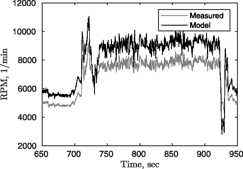The relative error between the expected RPM $\hat{n}$ and the measured RPM n is about 20%. We found similar accuracies when analysing wind-tunnel measurement data. The model can be significantly improved by adjusting (i.e. lowering) the K_V value to account for the additional load conditions. However, implementing such an adjustment requires measuring the actual RPM in which case the ESC/BLDC model is not needed anyways. Thus, we recommend using the manufacturers K_V value, if RPM measurements are not available. Note that this model fails to represent fast decelerations, because in this case the propellers are in a wind-milling state and are accelerated by the inflow, which is not represented in the model.

Figure 8.

BLDC/ESC model. RPM: revolutions per minute.

The propeller model (8) consists of two constants K₁ and K₂. We assume that K₁ can be accurately determined from the static motor model (6). K₂, however, has to be either measured in wind-tunnel tests or determined using analytical methods. The approximation of K₂ as a function of the propeller diameter and propeller pitch given in equation (9) can be used as a first approximation if no other data are available. It is, however, not clear if over- or underestimation occurs. In our experience, K₂ only becomes significant at high airspeeds, at which point the rudder effectivity usually is high enough for the rudders to act as the primary control surface.

In summary, we expect the motor model to be sufficiently accurate with a tendency to overestimate the propeller effectivity. Thus, reffering to Figure 2, this should result in fully damped system dynamics.

Dynamic actuator model

The rate-limited first-order lag model used to model servo motors has three parameters: the rate limit ${\dot{u}}_{\max}$ , the time constant T and the delay τ. Typically, servo manufacturers only specify a ‘servo speed’ given as the time needed to travel a certain angular distance. Unfortunately it is not clear how exactly this speed specification relates to the servo parameters given above. Directly using the servo speed as the rate limit does certainly not result in an accurate model. To find the model parameters, dedicated tests have to be conducted, for example, by probing the internal potentiometer output of the servo motor as suggested in Bronz et al.³ As an alternative, we built a servo testbench, which also permits us to study the frequency-dependent behaviour of a servo motor. Figure 9 shows the commanded angle and the measured servo angle over time. As is clearly visible, the servo motor cannot reach the commanded amplitude at this frequency. The rate limit thus leads to an attenuation of the input signal. There is also a phase delay between the commanded and the actual signal. The attenuation and the phase delay give rise to a Bode plot, where we define the phase shift as the value which provides the best-fit between input and output signal.

Figure 9.

Servo dynamics at high frequencies.

Figure 10 shows an example Bode plot obtained by running the test displayed in Figure 9 for many different frequencies. It is clear that a low-order linear servo model cannot capture the magnitude and phase behaviour of the nonlinear servo model. The sharp edge in the magnitude plot is related to the nonlinear effects of the rate limit. The time constant T of the servo actually has little impact on the overall modelling accuracy. How and if this actuator model should influence the design of outer loop controllers still needs to be investigated. As a comparison, Figure 10 also shows an approximation of the nonlinear servo model using a first-order lag, where the time constant is chosen such that it matches the edge frequency of the nonlinear servo model. In terms of designing outer loop controllers, such an approximation might serve as a useful abstraction of the nonlinear dynamic model to still allow the application of linear control methods.

Figure 10.

Bode plot of servo dynamics.

In summary, the actuator models presented here are able to capture the dynamic behaviour of the real actuators well. In case of electric motors, simple linear models seem to sufficiently capture the relevant dynamics. In the case of servo motors, the model parameters are hard to derive based on the typical manufacturer specifications. To apply the analysis summarised in Figure 3, suitable alternative (linear) actuator models need to be derived.

Results

The previously described models were used to model the actuators of a small tiltwing aircraft (wingspan $\approx$ 1.4 m, see Figure 11) as described in previous work.⁴

Figure 11.

Tiltwing aircraft.

In the nominal case, it can be shown² that the dynamics of the closed INDI control loop from the commanded angular accelerations ${\dot{ω}}_{c}$ to the actual angular accelerations ω are equal to the relevant actuator dynamics A(z). To analyse the INDI controller performance and thus at the same time the modelling fidelity, we use filtered versions (index f) of the control signal ${\dot{ω}}_{c f}$ and the actual accelerations ${\dot{ω}}_{f}$ . For example, the roll accelerations ${\dot{p}}_{f}$ and the corresponding command signal ${\dot{p}}_{f c}$ are calculated as shown in equations (12) and (13).

{\dot{p}}_{c f} = A (z) \cdot H (z) \cdot \frac{1}{z} \cdot {\dot{p}}_{c}

(12)

{\dot{p}}_{f} = \frac{z - 1}{T_{s} z} \cdot H (z) \cdot ︸ \underset{p_{meas .}}{\frac{1}{z} \cdot p}

(13)

If the actuator dynamics A(z) are modelled correctly, ${\dot{ω}}_{c f}$ should be equal to ${\dot{ω}}_{f}$ , which can be determined in-flight and thus offers a convenient method to assess the modelling fidelity in flight tests.

Figure 12 shows the results of a hover flight with the example tiltwing aircraft (see Figure 11) and the previously described actuator models. It is clear that the expected behaviour, namely, the relevant actuator dynamics A(z), is achieved by the controller. Errors in the actuator effectivity would directly result in a damping or amplification of the actual accelerations ${\dot{ω}}_{f}$ w.r.t the commanded accelerations ${\dot{ω}}_{c f}$ . Errors in the actuator dynamics would be visible as a time delay between these two signals.

Figure 12.

Performance of angular acceleration control loop.

On top of these closed-loop dynamics of the angular accelerations, simple proportional-derivative control can achieve a satisfactory attitude controller performance (as described in previous work⁴). In particular, no further gain scheduling is needed in the outer control loops for the example aircraft. Figure 13 shows the attitude controller performance (here reduced to roll- and pitch angle) over the entire flight envelope of the example tiltwing aircraft. Since the attitude controller is built on top of the angular acceleration controller, this shows that the chosen modelling approach is effective in achieving the required fidelity.

Figure 13.

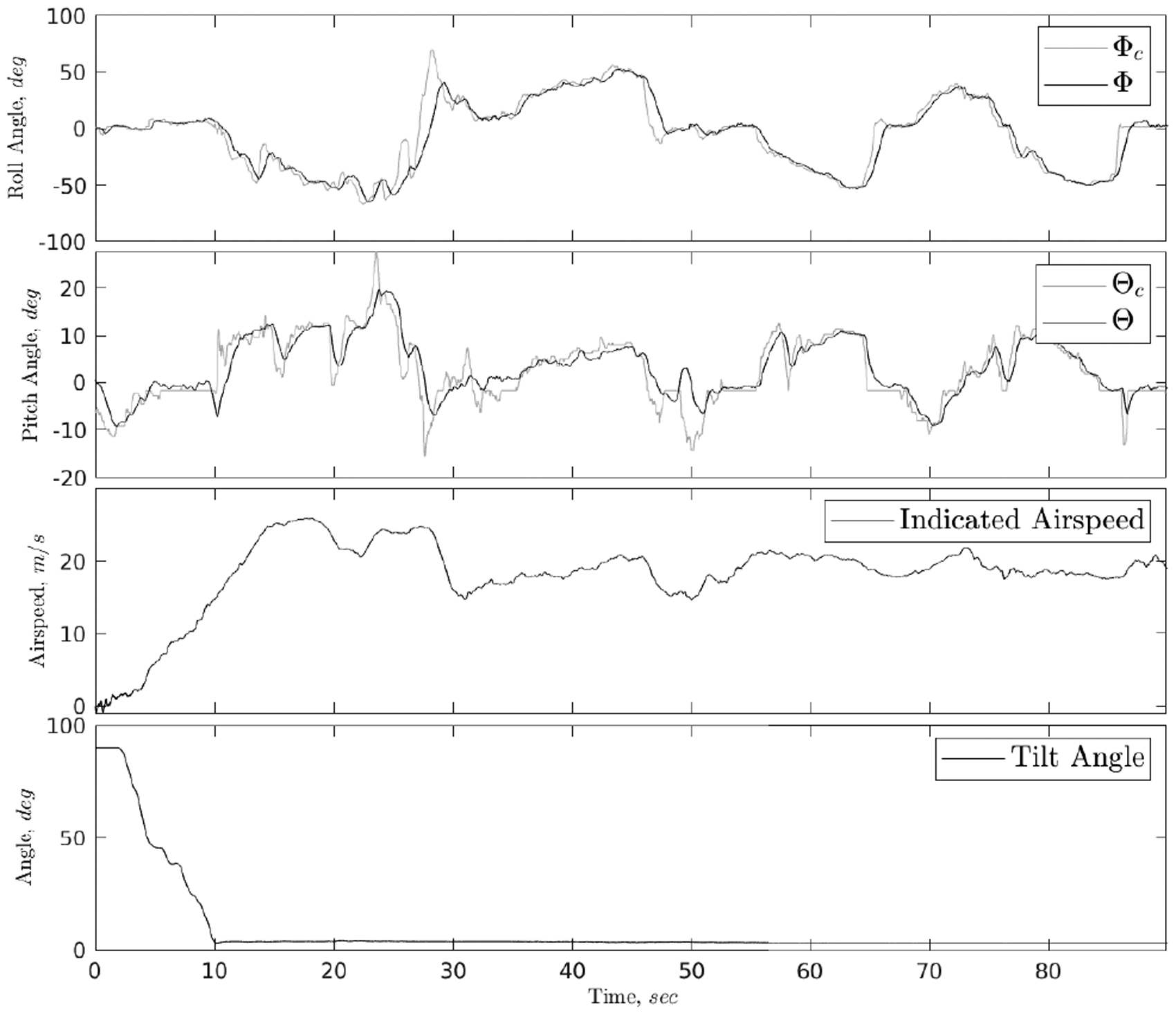
Performance of attitude control loop.

Conclusion

This paper presented our approach to modelling actuators for use in the framework of INDI. First, by studying the effects of modelling uncertainty on the poles of the closed-loop system, the robustness properties of INDI controllers were analysed. We confirmed the known stability properties of INDI but found that the uncertainty bounds of acceptable closed-loop performance are (of course) much tighter. With that in mind, we then considered the typical actuator elements found in small electric aircraft, namely, electric motors with propellers and rudders actuated by servo motors. We derived suitable models for these elements, trying to rely as much as possible and easily obtainable information.

In the following analysis, we assessed the resulting model fidelity using real flight data or measurements where possible. Special consideration was given to typical servo models, which feature a nonlinear rate-limit element. We discussed some effects of this nonlinearity, though further works needs to investigate how and if these nonlinearities should be considered in the design of outer loop controllers. Finally, flight test results could confirm that the chosen modelling approach is effective in achieving satisfactory attitude controller performance for an example tiltwing aircraft.

Footnotes

Declaration of conflicting interests

The author(s) declared no potential conflicts of interest with respect to the research, authorship, and/or publication of this article.

Funding

The author(s) received no financial support for the research, authorship, and/or publication of this article.

ORCID iD

F Binz

Note

a. APC 10x3.8 Slow Fly.

References

Sieberling

Chu

Mulder

JA.

Robust flight control using incremental nonlinear dynamic inversion and angular acceleration prediction. J Guid Control Dyn 2010; 33: 1732–1742.

Smeur

EJJ

Chu

de Croon

GCHE.

Adaptive incremental nonlinear dynamic inversion for attitude control of micro air vehicles. J Guid Control Dyn 2016; 39: 450–461.

Bronz

Smeur

Garciade de Marina

, et al. Development of a fixed-wing mini UAV with transitioning flight capability. In: 35th AIAA applied aerodynamics conference, aviation forum, Denver, CO, USA, 2017. DOI: 10.2514/6.2017-3739.

Binz

Islam

Moormann

Attitude control of tiltwing aircraft using a wing-fixed coordinate system and incremental nonlinear dynamic inversion. In: 10th international micro air vehicle competition and conference, Melbourne, Australia, 2018.

Bacon

Ostroff

AJ.

Reconfigurable flight control using nonlinear dynamic inversion with a special accelerometer implementation. In: AIAA guidance, navigation, and control conference and exhibit, Denver, CO, USA, 2000. DOI: 10.2514/6.2000-4565.

Binz

Hartmann

Moormann

Nonlinear model predictive flight path control for an unmanned powered paraglider. In: Euro GNC 2017 - 4th CEAS specialist conference on guidance, navigation & control, Warsaw, Poland, 2017.

Smeur

EJJ

de Croon

GCHE

Chu

Cascaded incremental nonlinear dynamic inversion for MAV disturbance rejection. Control Eng Pract 2018; 73: 79–90.

van’t Veld

van Kampen

Chu

Stability and robustness analysis and improvements for incremental nonlinear dynamic inversion control.In: 2018 AIAA Guidance, Navigation, and Control Conference, Kissimmee, Florida, USA, 2018. DOI: 10.2514/6.2018-1127.

Brandt

Deters

Ananda

, et al. UIUC propeller database, https://m-selig.ae.illinois.edu/props/propDB.html (2019, accessed 17 September 2020).

10.

APC Propeller Performance Data, www.apcprop.com/technical-information/performance-data/ (accessed 17 September 2020).

11.

McCrink

Gregory

JW.

Blade element momentum modeling of low-Re small UAS electric propulsion systems. AIAA Aviat 2015;: 54: 1–23.

Actuator modelling for attitude control using incremental nonlinear dynamic inversion

Abstract

Keywords

Introduction

Effects of modelling uncertainty

Poles of the INDI controller

Actuator models

Static actuator effectivity models

Motors

ESC/Brushless Direct-Current Electric Motor (BLDC) model

Propeller model

Rudders

Dynamic actuator models

Analysis

Motor model

Dynamic actuator model

Results

Conclusion

Footnotes

Declaration of conflicting interests

Funding

ORCID iD

Note

References