Sage Journals: Discover world-class research

Abstract

Recent advances in multi-rotor vehicle control and miniaturization of hardware, sensing, and battery technologies have enabled cheap, practical design of micro air vehicles for civilian and hobby applications. In parallel, several applications are being envisioned that bring together a swarm of multiple networked micro air vehicles to accomplish large tasks in coordination. However, it is still very challenging to deploy multiple micro air vehicles concurrently. To address this challenge, we have developed an open software/hardware platform called the University at Buffalo’s Airborne Networking and Communications Testbed (UB-ANC), and an associated emulation framework called the UB-ANC Emulator. In this paper, we present the UB-ANC Emulator, which combines multi-micro air vehicle planning and control with high-fidelity network simulation, enables practitioners to design micro air vehicle swarm applications in software and provides seamless transition to deployment on actual hardware. We demonstrate the UB-ANC Emulator’s accuracy against experimental data collected in two mission scenarios: a simple mission with three networked micro air vehicles and a sophisticated coverage path planning mission with a single micro air vehicle. To accurately reflect the performance of a micro air vehicle swarm where communication links are subject to interference and packet losses, and protocols at the data link, network, and transport layers affect network throughput, latency, and reliability, we integrate the open-source discrete-event network simulator ns-3 into the UB-ANC Emulator. We demonstrate through node-to-node and end-to-end measurements how the UB-ANC Emulator can be used to simulate multiple networked micro air vehicles with accurate modeling of mobility, control, wireless channel characteristics, and network protocols defined in ns-3.

Keywords

Unmanned aerial vehicle swarms multi-agent planning and control wireless networks emulation ns-3 MAVLink

Introduction

Micro-aerial vehicle (MAV) swarms are poised to enable breakthroughs in a variety of applications including surveillance, emergency first response, package delivery, environmental monitoring, and precision agriculture. However, designing and deploying multiple networked MAVs poses numerous inter-disciplinary challenges¹ because the communications and networking problems cannot be explored independently of problems in multi-agent planning and control. Unfortunately, there is currently no suitable testbed framework for researchers to use in order to holistically investigate these problems in simulation and easily transition to experimentation. To address this gap, we have spent the last few years developing the University at Buffalo’s Airborne Networking and Communications Testbed (UB-ANC).^2,3 UB-ANC^a is a flexible and low-cost multi-agent airborne networking and communications research platform that combines aerial vehicles capable of autonomous flight with (i) sophisticated command and control capabilities and (ii) the ability to experiment with common wireless standards, such as IEEE 802.11 (Wi-Fi) and IEEE 802.15.4 (Zigbee), or custom protocols implemented on software-defined radios.

Although actual system implementations are recognized as being crucial for demonstrating and evaluating airborne networks in real-world operating environments,^4–6 there are numerous challenges associated with conducting field tests with a swarm of multiple networked drones. On the technical side, the systems and software on each drone – including the network protocol stack, the mission planning algorithms, and the flight-controller – are very complex. Developing and integrating them requires lots of testing to ensure their correct operation. While each component can be tested independently, the fully integrated system currently needs to be tested in the field. However:

Conducting field tests requires having multiple flight-ready drones. This is not always possible because drones require frequent and time-consuming maintenance, especially when experimenting with large numbers.

Conducting field tests requires good weather conditions (no rain, low wind, etc.).

Conducting field tests requires well-trained personnel for safety and to satisfy FAA Part 107 regulations.^b

A majority of drones (i.e. multi-rotors) have limited battery lifetimes (<30 min), mandating a large supply of batteries and frequent charging interruptions during experimentation.

A popular approach to ease deployment challenges is the use of simulation/emulation. There are several simulators that address parts of the challenges listed above. Robotics simulation packages allow for simulation of individual drones with realistic physics, but make it hard to simulate/emulate multiple drones at the same time. Network simulators support the simulation of wireless networks but do not make it easy to simulate the interaction between networking, mission planning, and control. We looked through several possibilities and found it challenging to assemble a set of tools that would help us test drone networking applications in simulation and translate them to practice with ease.

To address the aforementioned challenges and fill the gaps in existing tools, we developed the UB-ANC Emulator,^7,8 which is a simulation framework that combines multi-MAV planning and control with high-fidelity network simulation and provides seamless transition to actual drones. The UB-ANC Emulator’s key characteristics are as follows:

The UB-ANC Emulator is designed using open-source software components borne out of the popular hobby drone movement. Therefore, it is easily usable with many off-the-shelf and custom-built drones.

It is designed using the same software that executes on actual drones including any mission planning algorithms, a software-in-the-loop (SITL) simulator of the flight controller, the protocol and application program interfaces (APIs) for communicating with the flight controller (i.e. the Micro Air Vehicle Communication Protocol (MAVLink⁹)), and APIs for sending and receiving data over the network.

It provides the same data logging capabilities as the actual drones and the ability to monitor the emulated mission via real-time visualization using open-source ground control stations, such as APM Planner¹⁰ and QGroundControl.¹¹

It is designed to be both modular and extensible, and can therefore be extended to easily incorporate other network elements, planning algorithms, sensors, and flight controllers that use the MAVLink protocol.

It provides an API for integrating a high-fidelity network simulator. We use this API to integrate the discrete-event network simulator ns-3¹² into the emulator.

Although we focus on emulating quadrotors in this paper, the UB-ANC Emulator can emulate any MAVLink compatible vehicle including fixed-wing planes, helicopters, multirotors, rovers, boats, and submarines.

The UB-ANC Emulator is available as open-source at https://github.com/jmodares/UB-ANC-Emulator.

The remainder of this paper is organized as follows. In the next section, we discuss related work. In the ‘Software architecture’ section, the UB-ANC Emulator’s software architecture is described. Then, the emulator’s accuracy is demonstrated. In the ‘Network simulator integration’ section, we introduce an API that allows us to integrate a network simulator into the UB-ANC Emulator and illustrate its usage with ns-3. This is followed by a section that validates the network simulator integration. The conclusions are presented in the final section.

Related work

Deploying and experimenting with MAV swarms require expertise in several areas including multi-agent systems, robotics, and mobile ad-hoc and wireless networks. A lot of research in each of these areas has been fueled by powerful simulation environments.

Multi-agent systems have been studied for several decades with significant interest in modeling coordination and swarm behavior. Swarm and MASON allow simulation of hundreds of agents and their interaction. Swarm¹³ was built in the early 1990s and fueled the beginning of swarm research. MASON¹⁴ is written in Java, and distinguishes between modeling and visualization allowing for easy attachment and detachment during runtime, and enabling algorithm developers to easily debug swarm applications. Simbeeotic¹⁵ simulates swarms of MAVs with full physics using the JBullet physics engine. Several multi-UAV applications have been demonstrated on it. The open-source aerospace multi-agent simulation environment (OpenAMASE^c) allows for command and control of multiple UAVs. AMASE UAVs feature a simulated autopilot and can be equipped with gimbaled and fixed sensors. The platform supports simulated footprint analysis for target detection and includes line-of-sight calculations for obscuration of sensors by terrain. The aforementioned platforms allow simulation of a large number of agents but require one to create a model of the aerial vehicle before it can be simulated, so it is not easy to represent an off-the-shelf aerial vehicle in them. As such, they do not support seamless transition from simulation to deployment on actual drones. Additionally, multi-agent system simulators generally do not support high-fidelity network simulation, despite the fundamentally unreliable nature of the (lossy) wireless channel and the potential negative consequences of communication failures in such systems.^16,17

There has been a lot of interest from academia and industry in all aspects of robotics. A lot of this research is powered by strong simulation support. In the 2000s, Player-Stage¹⁸ was one of the first simulators that allowed for development of controllers that could be deployed on robots, as well as in simulation. Stage is a 2.5D simulation engine that provides realistic physics simulation. ROS¹⁹ evolved the server–client architecture used for communication between controller nodes in Player-Stage to a peer-peer distributed architecture. It is distributed with Gazebo,²⁰ a realistic 3D simulator with full 6-DoF physics simulation. While these systems form excellent simulation/emulation platforms for robotic algorithms, they are challenging to scale up because, as the number of robots grow in simulation, the time to simulate grows due to the complexity associated with simulating full physics. It is near impossible to simulate tens to hundreds of agents interacting in such systems. Additionally, robotics simulators generally do not support high-fidelity network simulation.

Many advances in both wired and wireless networking have been driven by simulation tools. ns-2²¹ and ns-3¹² are discrete-event network simulators that have been used both in the classroom and by researchers for over a decade. Opnet,²² Glomosim,²³ and OMNet++²⁴ have also been used for wireless networking research and education. Such simulators are useful for prototyping and comparing protocols at different layers of the network protocol stack²⁵ and have played a key role in understanding airborne networks. Le et al.²⁶ simulate a reliable user datagram protocol for airborne networks in OPNET Modeler v14.5. Namuduri et al.²⁷ discuss cyber-physical aspects of airborne networks and use ns-2 to study average path durations under different node velocities, hop counts, and node densities. Javaid et al.²⁸ build a system called UAVSim on top of OMNet++ to analyze cyber-security threats in UAV networks. Such simulators provide realistic networking including queuing behaviors, protocol interaction, and channel modeling. They do not, however, model physical movement of individual nodes and related dynamics accurately, support realistic command and control, or enable seamless transition from simulation to experiment on actual drones.

While there are several platforms that address aspects of the development of MAV swarms, our survey did not find a platform that adequately combines multi-MAV planning and control with high-fidelity network simulation. We also believe that enabling simulation/emulation of aerial vehicle platforms that have evolved from popular open-source standards will allow for quick, seamless, and low-cost deployment on real systems. The UB-ANC Emulator, integrated with ns-3, represents our effort to bridge the gap between research and deployment on such systems.

In our prior work, we presented a demo of the UB-ANC Emulator in Modares et al.,⁸ focused on its behavioral and network simulation capabilities in Modares et al.^7,29 respectively, and used it to simulate an energy-efficient coverage path planning algorithm in Modares et al.³⁰ In this paper, we aggregate and extend our prior work with new insights, and new simulation and experimental results.

Software architecture

Figure 1 provides a high-level diagram of the UB-ANC Emulator’s architecture, which comprises three main components: the Emulation Engine, MAV Object, and UB-ANC Agent. The Emulation Engine is the core of the emulator: it coordinates various tasks, and instantiates and interfaces with one MAV Object per simulated MAV. Each MAV Object contains the UB-ANC Agent, which hosts the mission behavior and can be directly executed on the drone. Each UB-ANC Agent interfaces with three other modules: a flight controller, a network server, and a sensor server. An open-source SITL simulator³¹ is used to simulate the flight controller. The SITL simulator can be connected to an open-source GUI such as APM Planner¹⁰ to visualize and monitor the emulated MAVs. A visualization of APM planner is shown in Figure 3.

Figure 1.

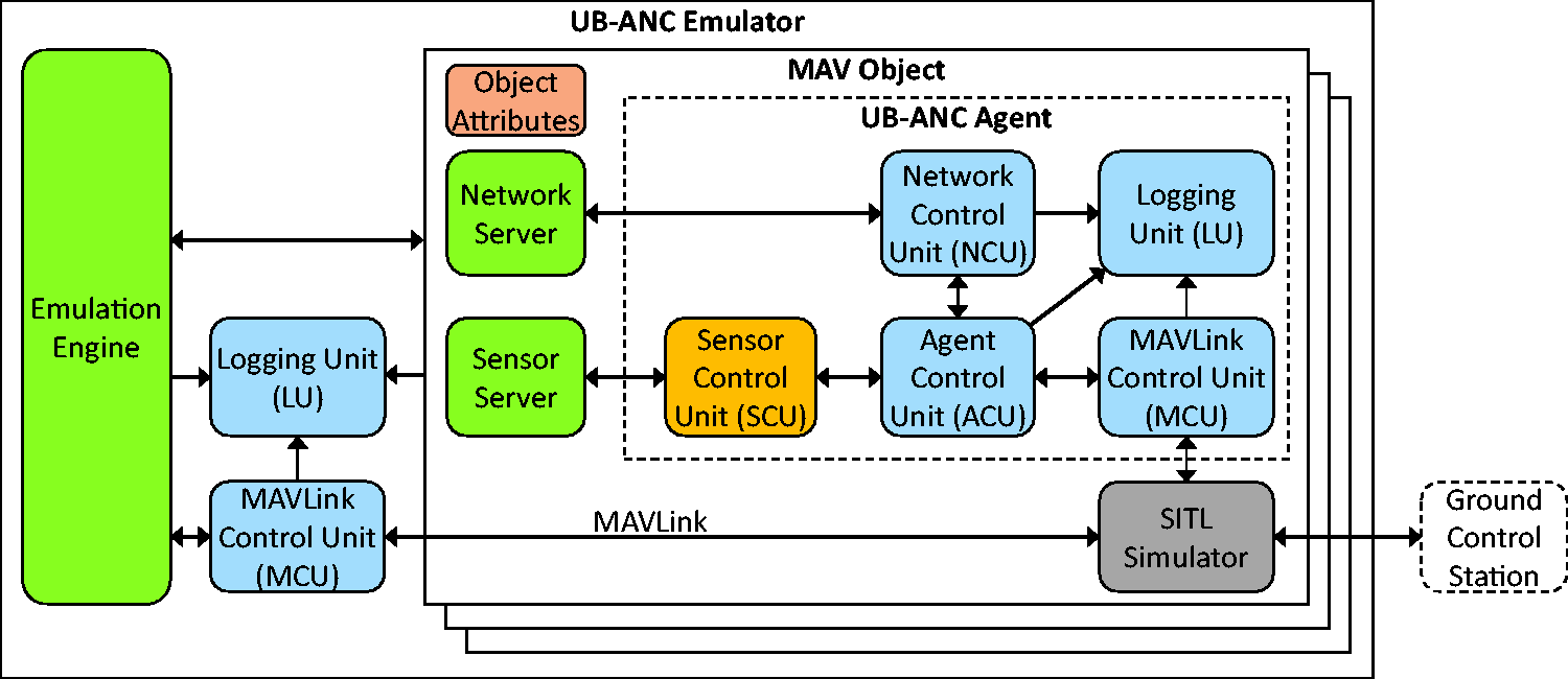
The UB-ANC Emulator’s software architecture.

Before we describe each component of the emulator in detail, we highlight the key features of its design:

Modularity: The UB-ANC Emulator is designed to be modular. Each component has a well-defined task so that it can be easily modified and debugged. Each module also has well-defined interfaces to interact with other modules. Consequently, we can instantiate new sensor behavior, network protocols, and different flight controllers by modifying the individual modules.

Extensibility: The modules in Figure 1 have been designed for easy extensibility. Clearly defined interfaces separate each of the modules. This allows for developers to create new modules for novel hardware components. For instance, the MAVLink component can be modified to integrate a new behavior for a specific drone.

Ease of deployment: The UB-ANC Emulator is easy to set up and run. It is written in C++ and leverages the Qt cross-platform development framework so that it can be ported to various platforms such as Windows and Linux. Moreover, after verifying a new flight controller or mission planning algorithm in emulation, this functionality can be deployed on the actual hardware without modification.

Adherence to popular open-source standards: The UB-ANC Emulator is designed to support MAVLink compatible flight controllers, which support a variety of autonomous vehicles including fixed-wing planes, helicopters, multirotors, rovers, boats, and submarines. The MAVLink protocol is an open standard that is supported by many popular flight controllers including Pixhawk, NAVIO, Erle-Brain, and Intel’s Aero.^d We also leverage popular open-source tools built by the hobby community for visualization and logging.

As noted above, the UB-ANC Emulator is written in C++ and leverages the Qt cross-platform development framework.^e We chose Qt for several reasons. First, it makes it easy to maintain a modular design with components that have separate tasks. In particular, using Qt’s signals and slots mechanism, components can communicate by emitting signals and capturing other components’ signals using slots. Second, the majority of components that the UB-ANC Emulator uses come from existing open-source projects that are based on Qt. Third, Qt makes it easy to port the UB-ANC Emulator to other platforms.

UB-ANC agent

The UB-ANC Agent comprises five components: the agent control unit (ACU), the network control unit (NCU), the sensor control unit (SCU), the MAVLink control unit (MCU), and the logging unit (LU). The ACU is the “brains” of a UB-ANC drone: it contains the mission planning logic and interfaces through well-defined APIs with (i) the NCU to talk with different network elements; (ii) the SCU to talk with different sensors; (iii) the MCU to talk with different flight controllers; and (iv) the LU to log status information. Importantly, the UB-ANC Agent can be moved from simulation to experiment (i.e. actual deployment on drones) without modification. We will now describe the components of the UB-ANC Agent in detail.

ACU

The ACU is responsible for any mission that the drone is supposed to complete. It includes the internal logic for deciding what commands to send to the flight controller (through the MCU) and what information to send to other nodes (through the NCU) to accomplish its mission. In general, the mission planning logic can make decisions based on local state information and information received from other nodes. Note that GPS-based flight controllers, such as the Pixhawk, accept GPS waypoints as input for control. Thus, the ACU’s internal planning logic is primarily responsible for deciding which GPS waypoints to visit over time.

MCU

The ACU uses the MCU to send commands to the flight controller. In order to send/receive commands (or messages) to/from the controller, the MCU uses the MAVLink messaging protocol.⁹ The MCU allows us to interface with the flight controller in multiple ways (e.g. TCP or serial link) and supports connections to a variety of MAVLink compatible flight controllers.

NCU

The ACU uses the NCU to communicate with other MAVs and with ground control stations (if any). MAVs may exchange different types of information, ranging from sensing to command and control. Every MAV has the ability to send commands and state information to other MAVs in the network, thereby enabling the deployment of both centralized and distributed mission planning algorithms. The NCU allows us to switch network elements while keeping the rest of the system the same. Therefore, we can test the same planning algorithms with different network technologies (e.g. Wi-Fi, Zigbee, or a custom communication interface via GNU Radio, for example), allowing for fair comparison across them.

SCU

The ACU uses the SCU to read sensor data. Currently, the SCU supports a custom sensor module that can measure the current draw of different system components (e.g. motors). In the future, we will extend the SCU to support other types of sensors, such as proximity sensors and cameras.

LU

Experimenting with a single drone already involves several interacting components, yet it is much more complex when multiple drones are executing a mission together. Logging and tracking the sequence of events is an important aspect of simulating such scenarios for easy debugging and understanding. Each UB-ANC agent has an LU that allows for numerous internal parameters to be logged and tracked. They include, but are not limited to, GPS coordinates, MAVLink messages, drone velocity, received signal strength indicator (RSSI), packet information (e.g. packet ID, size, source ID, destination ID), etc. We leverage Qt’s logging mechanisms for this purpose.

MAV object

The MAV object component represents a MAV in the emulator. Along with an instance of the UB-ANC Agent, it contains an instance of the SITL simulator,³¹ which simulates the flight controller that interfaces with the UB-ANC Agent via MAVLink messages. The MAV object also creates network server and sensor server components. These provide a level of indirection and abstract the individual network and sensor elements present in simulation, which allows for progressive emulation. For example, we can simulate the drone behavior but connect the computer to a wireless network allowing for network experimentation while simulating the rest of the system (see the ‘Extensibility’ section). Similarly, we can simulate any combination of the individual components while testing the rest in experiment. In simulation, there are several private properties of sensing and communication, such as sensing and communication ranges, and communication and sensing models, which are held in the MAV object. These are shown as object attributes in Figure 1 and are communicated with the emulation engine for reasoning across simulated drones.

Emulation engine

The emulation engine is the central housekeeper for the UB-ANC Emulator. It is responsible for instantiating MAV objects (one for each emulated MAV), providing network communication across MAVs, and sensing performed by individual MAVs in simulation. Based on the MAV positions and simulation setup, it delivers messages to/from MAVs within communication range (as determined by the Object Attributes and the network modality) and sensing information to individual MAVs.

SITL

The SITL³¹ simulator is an open source project that allows you to run the flight dynamics model of a wide variety of vehicle types, including multirotor aircraft, fixed wing aircraft, and ground vehicles, without any hardware. Depending on what the simulator is connected to, we can vary the degree of physics being simulated and thereby vary the degree of realism of the simulation. For instance, it is possible to connect it to the commercial flight simulator X-Plane 10 to simulate full physics.^f This is a key design choice allowing us to trade off scalability and fidelity based on the simulation requirements.

Drone emulation evaluation

In this section, we describe the experiments and simulations that we perform to evaluate the accuracy and extensibility of the UB-ANC Emulator. Figure 2 shows a close up of one of the custom-built UB-ANC drones that we used to gather our experimental results. Figure 3 shows the emulator connected to APM Planner for visualization.

Figure 2.

A UB-ANC Drone with a custom frame, Pixhawk flight controller, Raspberry Pi 2 board, custom power sensor module, and 10,000 mAh battery. The drone weighs approximately 3 kg and achieves up to 30 min of flight time.

Figure 3.

APM Planner visualization for UB-ANC Emulator.

A major challenge in analyzing a simulator is determining its accuracy with respect to reality. To this end, many robot simulators simulate full physics. However, this limits their scalability in the number of robots simulated. Our simulator simulates MAVlink-compatible robots. The MAVlink protocol communicates in terms of events. As an indicator of accuracy, we measured the time between events on a MAV and compare them to the corresponding times in the simulator. These results are presented in the ‘Accuracy’ section. In the ‘Extensibility’ section, we connect two USRPs to our simulator and use them to communicate between two simulated MAVs to demonstrate network extensibility. In the ‘Simulating other parameters’ section, we measure energy consumption, flight speed, and barometric pressure on a real drone and compare the real data against that obtained in the emulator. This demonstrates that the UB-ANC Emulator can simulate various parameters of interest. Finally, in the ‘Minimum energy path planning’ section, we show experimental and simulation results for two sophisticated path planning algorithms. These results further highlight the accuracy of the simulator with respect to reality.

Accuracy

To show the accuracy of the UB-ANC Emulator with respect to MAV experiments, we set up three UB-ANC Drones (MAVs) on UB’s North Campus to perform a simple “takeoff, loiter, and land” mission. We also execute the same mission in the UB-ANC Emulator. The mission begins when MAV 1 is armed. MAV 1 then takes off to an altitude of 5 m, flies east for 5 m, and then loiters (hovers) for 20 s before landing. When MAV $i \in {1, 2}$ first starts to loiter, it sends a command to MAV i + 1 to takeoff, loiter, and land in the same pattern. We repeat this three-MAV mission for five rounds. Note that, although the UB-ANC Drones are capable of completing more complicated missions, we have selected a relatively simple mission for illustration in this section. We present a more sophisticated path planning mission in the ‘Minimum energy path planning’ section.

Figure 4 compares several important quantities that we measured in our experiments and simulation. In Figure 4, time 0 corresponds to the time when MAV 1 is armed. Figure 4(a) shows the average (markers) and standard deviation (error bars) of the time at which several key events occur at each MAV (ARM, LAND, and DISARM) over the five experimental and simulation rounds. For MAV 1, the ARM event represents the time that it starts to spin-up its motors to takeoff. For MAV $i \in {2, 3}$ , the ARM event corresponds to a sequence of four events: (i) MAV i–1 sends a command to MAV i to start its mission; (ii) MAV i receives the command from MAV i–1; (iii) MAV i arms its motors; and (iv) MAV i initiates takeoff. For all three MAVs, the LAND event represents the time at which the autonomous landing mode is initiated, and the DISARM event represents the time at which the MAV has landed and disarms its motors, signifying the completion of its mission. Figure 4(b) and (c) shows each MAV’s longitude deviation (from its initial starting position) and relative altitude (from the ground) over time, respectively. Note that we do not show the latitude because it is fixed for the duration of the mission.

Figure 4.

Emulation vs. experiments for a three-drone mission. (a) Events vs. time. (b) Longitude vs. time. (c) Altitude vs. time.

It is immediately apparent from Figure 4(a) to (c) that there is extra delay in the simulations compared to the experiments. To identify the source of this delay, we have partitioned the MAVs’ flight paths into four segments: arm-to-takeoff, takeoff-to-peak altitude, travel, and land-to-disarm. The average and standard deviation of the time required to complete each segment of the flight path for one MAV are plotted in Figure 5. Clearly, the arm-to-takeoff delay dominates the difference in measured time between simulation and experiment. Therefore, we conclude that it is primarily responsible for the extra delay observed in the simulation results. We believe that the MAV takes off faster in the experiments than in the simulations because of the so-called ground effect, which results in the propellers achieving better performance near the ground (i.e. producing more thrust per unit power) compared to flight further from the ground.^32,33 The delay is near constant in our measurements for each MAV, and can easily be incorporated into the simulation based on the exact MAV being used in an experiment.

Figure 5.

Potential sources of time lag between experiments and simulations for one drone.

In Table 1, we show the variance of the simulation and experimental data that is shown in Figure 4. Since the simulation itself is deterministic, the variance in the simulated event times is due entirely to background processes/computer load and is essentially negligible. Meanwhile, the variance in the experimental results are reasonably small given the many possible sources of deviation (e.g. wind variations in each round, GPS accuracy, and variation in the flight controller’s response to noisy accelerometer and barometer readings). In Table 2, we show the mean squared error (MSE) between the average experimental measurements and the average simulation measurements with and without compensating for the extra arm-to-takeoff delay that appears in the simulations. We see that, especially when accounting for the time lag, the MSE is quite small. This suggests that the emulator provides a good approximation for MAV experiments even though it does not simulate full physics.

Table 1.

Variance of experimental and simulation measurements across five rounds.

	MAV 1	MAV 2	MAV 3
Event Variance
Experiment	0.5460	0.1365	0.3598
Simulation	0.1082	0.0010	0.0009
Longitude Variance
Experiment	0.0138	0.0450	0.0346
Simulation	0.0133	0.0085	0.0252
Altitude Variance
Experiment	0.0281	0.0386	0.0474
Simulation	0.0119	0.0017	0.0013

MAV: micro air vehicle.

Table 2.

MSE between the average experimental measurements and simulation measurements with (measured) and without (shifted) the extra arm-to-takeoff delay that appears in the simulations.

	MAV 1	MAV 2	MAV 3
Event MSE	2.8070	3.3644	2.8117
Longitude MSE
Measured	0.3501	0.2286	0.1736
Shifted	0.1478	0.0085	0.0329
Altitude MSE
Measured	0.4678	0.5536	0.5065
Shifted	0.0463	0.0468	0.0317
Time shift	1.9937	1.7487	1.8305

MAV: micro air vehicle; MSE: mean squared error.

Extensibility

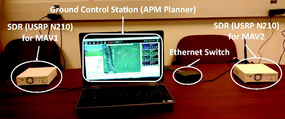
To show the extensibility of the emulator, we set up a “leader-follower” mission with five MAVs, where MAV 1 and MAV 2 communicate through two USRP N210 software-defined radios, while the other MAVs communicate in simulation. In this mission, MAV i + 1 follows 10 meters behind MAV $i \in {1, 2, \dots, 4}$ . This is accomplished by MAV i sending its GPS location to MAV i + 1 every 100 ms using a 74 byte packet. Figure 6 shows the setup for this demonstration.⁸ In the ‘Network simulator integration’ section, we further demonstrate the emulator’s extensibility by connecting it to ns-3 for high-fidelity network simulation.

Figure 6.

UB-ANC Emulator with two MAVs communicating over USRP N210 software-defined radios.

Simulating other parameters

In this section, to further demonstrate the flexibility and utility of the emulator, we simulate three other sensed values and compare them against real experimental data. All plots show data averaged across five trials of the “takeoff, loiter, and land” mission for one drone. Figure 7(a) shows the average total current draw across the drone’s four motors, which we measured using a custom-built current sensor module. This information is useful for energy-sensitive applications. For instance, in the ‘Minimum energy path planning’ section, we demonstrate how such information can be used for minimum energy path planning (MEPP). Figure 7(b) and (c) shows the flight speed and sensed pressure change, respectively (pressure is normalized to 0 on the ground). As in the ‘Accuracy’ section, we observe that the simulations yield accurate results with respect to the experiments, but with a small time delay. In Figure 7(c), we note that there is a spike in the pressure measurement on the actual drone at around 13 s into its flight. This corresponds to the dips in altitude observed in Figure 4 at about 13 s into each drone’s flight. We believe that this was caused by propeller backwash, which affected the flight controller’s barometric pressure readings.

Figure 7.

Simulation vs. experiment comparison of current draw, speed and pressure deviation on a drone. (a) Motor current draw (A). (b) Speed (m/s). (c) Pressure deviation (Pa).

MEPP

Using the aforementioned current sensor module, we took measurements to understand how a drone’s energy consumption during flight varies with respect to the distance traveled and direction changes.³⁰ Using the drone illustrated in Figure 2, we determined that energy consumption is approximately linear in the distance traveled (0.1164 J/m) and the turn angles (0.0173 J/deg). Although the exact measured values depend on the specific drone and flight controller, we observed similar trends across multiple tests on multiple quadrotors using Pixhawk flight controllers.

Using the linear energy consumption model, we formulated an MEPP problem.³⁰ The goal of this problem is to find a minimum energy path for a single drone to cover an arbitrary area with obstacles. The MEPP is similar to the well-known traveling salesman problem (TSP), but with additional terms in the optimization objective to account for the turning costs. To solve the problem efficiently, we modified the Lin-Kernighan Heuristic (LKH³⁴) for the TSP. While the conventional LKH only considers the distance traveled, we modify it to also account for the drone’s turning costs. We call our new algorithm LKH for Drones (LKH-D³⁰). We compare our LKH-D approach with the depth-limited search (DLS) algorithm with backtracking proposed in Barrientos et al.³⁵ Specifically, we use both algorithms to generate flight paths that cover the UB Stadium and evaluate them in the UB-ANC Emulator and on an actual UB-ANC Drone. We decompose the stadium into an 8 × 15 grid and create virtual obstacles that the drone must navigate around. We say that a grid cell is “covered” if the drone flies through its center and that the entire area is covered if all unobstructed grid cells are visited. We set the drone’s target speed to 5 m/s. The planned missions using DLS and LKH-D, visualized in APM Planner,^g are shown in Figure 8(a) and (c), respectively. The drone starts its mission at the top right corner of the field and follows the planned path, which returns it to its starting point.^h

Figure 8.

Satellite view of the UB Stadium and the planned coverage paths. Virtual obstacles are shaded with diagonal lines. (a) DLS path (planned), (b) DLS path (experiment), (c) LKH-D path (planned), (d) LKH-D path (experiment).

We observe that LKH-D determines a more efficient flight path with less turns than DLS, which allows the drone to cover the area at a higher average speed (because it does not need to slow down as frequently for turns), reduces the time that it requires to cover the area, and ultimately reduces its energy consumption. Specifically, LKH-D improves the overall energy consumed by 25% compared to DLS. This matches well with the simulation results in Table 3, which show that LKH-D achieves approximately 22% lower energy consumption than DLS. The close match between the simulation and experimental results further highlight the utility and accuracy of the UB-ANC Emulator.

Table 3.

Minimum energy path planning (MEPP) simulation and experimental results.

	Algorithm
	DLS		LKH-D
Metric	Sim	Exp	Sim	Exp
Energy (kJ)	118.38	111.1	92.56	83.9
Distance (m)	1043.8	1044.1	994.1	996.4
Turns (deg.)	2970	2970	1620	1620
Flight time (s)	389.5	391.6	291.1	293.7
Average speed (m/s)	2.67	2.66	3.41	3.39

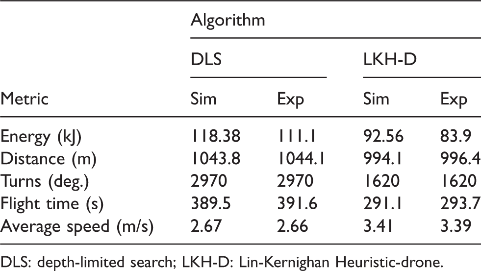
DLS: depth-limited search; LKH-D: Lin-Kernighan Heuristic-drone.

Network simulator integration

By default, the UB-ANC Emulator provides a simple network simulation, in which nodes can communicate with each other if they are within a given range. However, this does not accurately reflect the performance of a MAV network where communication links are subject to interference and packet losses, and protocols at the data link, network, and transport layers have a significant influence on network throughput, latency, and reliability. To overcome this limitation, our design choices included implementing our own network simulation or integrating an existing network simulator. As discussed in the ‘Related work’ section, there has been a lot of research on network simulation. After some exploration, we decided to integrate ns-3, which is a popular network simulator that has been designed for integration into testbeds and real network stacks. However, the same methodology could be applied to integrate other network simulator programs, such as EMANE.ⁱ

There are several challenges as well as design choices in integrating a network simulator such as ns-3 into the UB-ANC emulator. We briefly list them below:

Clock synchronization: ns-3 is a discrete-event simulator that processes events from a queue that are ordered in simulation time. In default operation, simulation time and clock time are not the same because simulation time jumps instantly from one simulated event to the next. However, the UB-ANC emulator simulates aerial vehicle behavior in real time.

Event synchronization: The UB-ANC Emulator simulates networks of MAVs. For this purpose, it translates agent behavior into MAVlink messages that are interpreted by the SITL simulator of the vehicle controller firmware. In short, several MAVlink events get processed in a per-agent manner on the individual SITL simulators. However, network simulators have their own event processing. To perform accurate simulation, these two event queues need to be synchronized frequently. This requires the network simulator to be informed of the relevant events in the UB-ANC Emulator in a timely manner.

Network activity synchronization: Algorithms implemented in the UB-ANC Emulator will often perform complex coordination behaviors that rely on the network. The primary goal of the network simulator integration is to synchronize the network activity between our emulator and the network simulator. This includes exception handling in cases of communication failure and/or external disturbances that affect communication.

Methodology for network simulator integration

For event synchronization, we forward all relevant events in the UB-ANC Emulator to the network simulator. Given the distributed nature of our implementation, we designed the UB-ANC Emulator to expose the three methods in Table 4 that allow the network simulator to interface with individual MAVs. These methods not only enable packet transmission and reception but also track MAV mobility. In this way, a network simulator can realistically model the connectivity and data transmission based on the MAVs’ positions.

Table 4.

API for integrating existing network simulation software into the UB-ANC Emulator.

Method	Description
netDataReady()	Signal that is emitted by a transmitter’s MAV object to transfer a packet to a network simulator
netSendData()	Slot that is used by a network simulator to transfer a packet to a receiver’s MAV Object
globalPositionChanged()	Signal that is emitted by the emulator’s MCU to inform a network simulator about a drone’s updated position

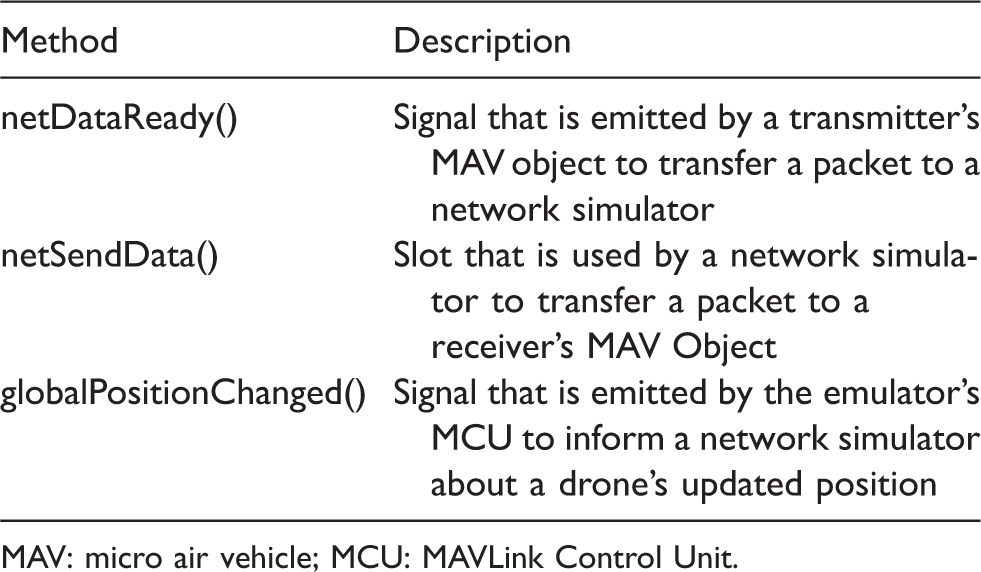
MAV: micro air vehicle; MCU: MAVLink Control Unit.

We now describe how the methods in Table 4 are used for packet transmission, packet reception, and MAV positioning.

Packet transmission

When the ACU wants to send a packet, it forwards the packet to the NCU, which puts it in a private queue called m_send_buffer. From there, the packet is forwarded to the sender’s corresponding MAV Object using interprocess communication (IPC) and the MAV object raises a signal called netDataReady(). This signal must be captured by the network simulator so that it can ingest the packet from the MAV object. Once ingested, the network simulator can process the packet, i.e. send it from the source node to its destination node using its internal representation of the network.

Packet reception

Once a packet is delivered to the destination node in the network simulator, it needs to be sent to the network server component of the destination node’s MAV object. This is achieved using the MAV object’s method (slot) netSendData(). The Network Server then forwards the packet to the NCU of the corresponding UB-ANC Agent component using an IPC mechanism. Subsequently, the NCU raises a signal called dataReady() to notify the ACU that there is a packet in the m_receive_buffer. The ACU then reads the buffer and processes the received packet.

Drone positioning

As described earlier, the drones’ positions need to be updated in the network simulator to match their positions in the emulator. When a drone’s position changes, the emulator’s MCU (shown in Figure 1) raises a signal called globalPositionChanged(). The Emulation Engine listens to the signal and passes it along to the network simulator which can then process it accordingly.

ns-3 integration

A high-level block diagram showing how we integrate ns-3 into the UB-ANC Emulator using the API described in the previous section is provided in Figure 9. In ns-3, a node represents a mobile transceiver that can send/receive packets to/from other nodes in a simulated network. As shown in Figure 9, each node contains an application layer, a network layer, a data link layer, a physical layer, and a mobility model. The application layer represents an application that runs on the mobile transceiver and can generate and consume network packets. The mobility model is responsible for positioning the mobile transceiver in the network over time.

Figure 9.

Block diagram illustrating how we have integrated ns-3 into the UB-ANC Emulator.

To simulate the MAV network, an ns-3 node (hereafter node) must be instantiated for each emulated MAV. Each node’s application layer handles packet transmit signals (netDataReady()) from the corresponding MAV object in the UB-ANC Emulator to initiate a packet transmission. Once a packet is ingested by the source node’s application layer, ns-3 sends the packet through its network stack to the destination node. Then, the destination node’s application layer uses the received packet slot (netSendData()) to send the packet to the node’s corresponding MAV Object in the emulator.

Clock Synchronization: As described earlier, a challenge to integrate ns-3 is that it uses a separate scheduler that needs to be synchronized in time with the UB-ANC Emulator’s scheduler. For this, we set ns-3 to use a real-time scheduler to lock the simulation clock with the CPU clock (and set real time as simulation time). This allows the two schedulers to be synchronized to the same clock.

Network simulation evaluation

We evaluate the integrated system for two scenarios: node-to-node and end-to-end connectivity. All of our network simulations are done using standard ns-3 models and protocols. For physical layer and channel modeling, we use the existing YansWifiPhy and YansWifiChannel models in ns-3, respectively, which are based on the “Yet Another Network Simulator” (YANS) model for IEEE 802.11b³⁶; at the medium access control (MAC) layer, we use the YANS IEEE 802.11 DCF model; for network layer routing, we use the built-in implementations of OLSR and AODV; and, at the transport layer, we use UDP. We transmit dummy data over the network to illustrate the platform’s basic functionality and the success of the integration. For our evaluations, we generate packet capture (pcap) files using ns-3 and analyze them offline using Wireshark (although other network analyzer tools can also be used).

Node-to-node connectivity

In order to evaluate the ns-3 integration at the link-level, we set up a channel measurement mission with two MAVs: MAV1 as the receiver and MAV2 as the sender. When the mission begins, MAV2 takes off to a 5 m altitude and then hovers while sending 1000 packets at an application (APP) layer rate of 1 packet/s. Each APP layer packet is 7 bytes, which increases to 93 bytes after adding MAC layer headers. After sending 1000 packets, MAV2 flies 5 m to the east and then hovers while sending another 1000 packets. It repeats this process a total of 20 times during the mission. We run this mission four times using direct sequence spread spectrum (DSSS) modulation with physical (PHY) layer data rates of 1 Mbps, 2 Mbps, 5.5 Mbps, and 11 Mbps. Figure 10(a) and (b) shows the number of packets received by MAV1 with respect to the received signal strength (RSS) and 3D Euclidean distance between the two MAVs, respectively. These results closely match those reported in Pei and Henderson on how Wi-Fi packet reception probabilities vary with RSS in ns-3. This validates our integration and demonstrates the correctness in event and clock synchronization.

Figure 10.

Packets received out of 1000 packets sent. (a) RSS (dBm) and (b) distance (m).

End-to-end connectivity

To evaluate the ns-3 integration on end-to-end packet delivery, we set up a network with seven MAVs as shown in Figure 12 with MAV1 as the source and MAV7 as the destination. We imagine that such an aerial ad-hoc network could be deployed in a disaster situation to enable first responders to communicate when conventional communication infrastructure is down. When the mission starts, all the MAVs take off to a 5 m altitude, fly to their respective positions, and circle 20 times at a speed of 5 m/s. The centers of adjacent circles are separated by either 40 $\sqrt{2}$ m or 80 m and each circle has a 20 m radius. Once it starts circling (approximately 200 seconds into the simulation), MAV1 sends packets to MAV7 (7 bytes at the APP layer; 93 bytes at the MAC layer). We run the test with APP rates of 1 packet/s (low) and 100 packets/s (high) with a PHY rate of 1 Mbps using DSSS for all nodes. Using this network, we compare the performance of two different routing protocols supported by ns-3, namely, ad hoc on-demand distance vector routing (AODV) and optimized link state routing (OLSR). Figure 12 shows the emulated network visualized by APM Planner.

Table 5 shows the transmitted and received data rates at the source (MAV1) and destination (MAV7), respectively, excluding overheads. The transmitted data rate at the source is greater under OLSR than AODV. At the same time, the received data rate is lower under OLSR than AODV. This is because OLSR’s HELLO_INTERVAL was set to 2 s (default) which was effectively less than the dynamic update rate in AODV. Consequently, OLSR’s routing table is occasionally out-of-date, so packets cannot reach MAV7 and must be retransmitted by MAV1. Figure 11 shows the number of packets sent by the source (MAV1) and received by the destination (MAV7) over time for different APP rates and different routing protocols. We can clearly see that the transmitted and received data rates vary over time with the MAVs’ positions and depend heavily on the routing protocol. Figure 13 shows the total amount of data and routing overheads (in bytes) transmitted by each MAV for different APP rates and routing protocols. We can clearly see the unequal traffic loads across the MAVs and that overheads account for a larger fraction of overall traffic at lower data rates. Finally, Figure 14 shows cumulative distribution functions (CDFs) of the end-to-end application layer delay between the source (MAV1) and the destination (MAV7). If an application layer packet never makes it to the destination, then we assign it an infinite delay; hence, the CDFs plateau before reaching 1. We observe that a higher fraction of packets are successfully delivered at 1 packets/s than 100 packet/s, but that the latter tend to achieve lower end-to-end delays. These results illustrate an important strength of emulation over real life experiments as delay measurements can be made relatively easily.

Table 5.

Transmitted and received data rates (bytes/s) at MAV1 and MAV7, respectively, excluding overheads.

	Low (1 packet/s)		High (100 packets/s)
	OLSR	AODV	OLSR	AODV
Source (MAV1)	127.71	123.93	11,881.94	11,735.35
Destination (MAV7)	86.07	89.13	6813.41	8524.34

OLSR: optimized link state routing; AODV: ad hoc on-demand distance vector; MAV: micro air vehicle.

Figure 11.

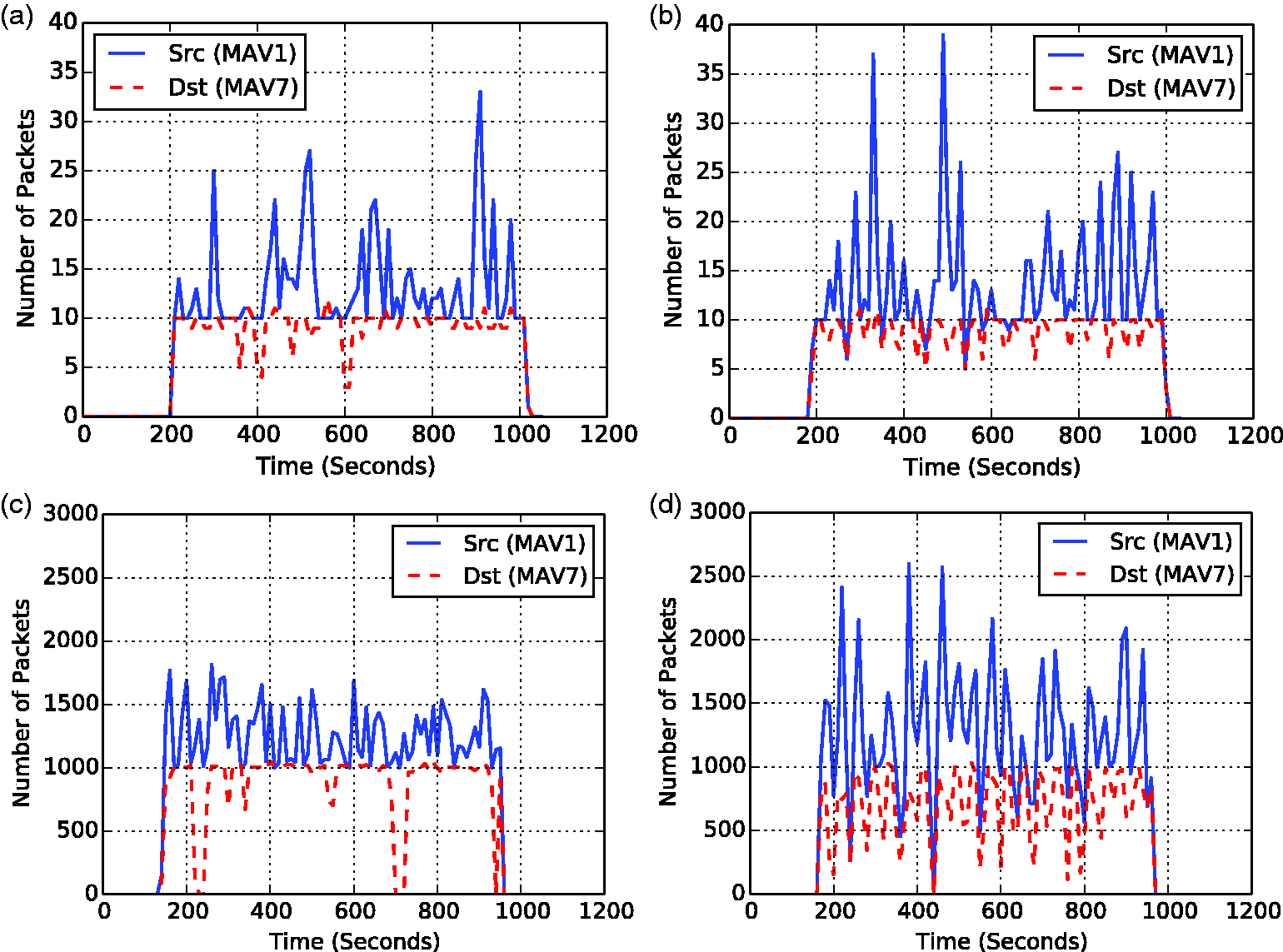
Number of data packets sent by MAV1 and received by MAV7 under different APP rates and routing protocols. (a) AODV routing with 1 packet/s APP rate, (b) OLSR routing with 1 packet/s APP rate, (c) AODV routing with 100 packet/s APP rate, (d) OLSR routing with 100 packet/s APP rate.

Figure 12.

A network of seven MAVs visualized using APM Planner. MAV1 is the source and MAV7 is the destination.

Figure 13.

Number of data and routing/overhead packets sent by each MAV under different APP rates and routing protocols. (a) 1 packet/s APP rate, (b) 100 packets/s APP rate.

Figure 14.

CDF of the end-to-end application layer delay.

Discussion

It is important to note that the default ns-3 models do not take into account the unique characteristics of aerial channels^37,38; however, they go far beyond the idealized communication models that are typically considered in multi-robot/multi-agent planning, control, and simulation (i.e. perfect communication within a predefined radius). In this context, one of the primary goals of our platform is to allow multi-robot systems researchers to evaluate the effectiveness of their planning algorithms under more realistic network conditions.¹⁷ In parallel, UAV communications and networking researchers have proposed many domain-specific protocols and models. If a user wants to use any of these sophisticated protocols/models in the UB-ANC Emulator, then they can do so by implementing them in ns-3. We believe that the UB-ANC Emulator can thus facilitate research at the frontiers and nexus of these research communities to advance swarm technology.

Conclusion

While there are many potential and emerging applications for MAV swarms, deployment and testing of such systems is extremely challenging because it requires experience in networking, software systems, robotics, mission planning, and control among others. In this paper, we presented the UB-ANC Emulator, which streamlines the design of MAV swarms and applications by allowing researchers and practitioners to first implement and test them in software, and then seamlessly transition them to actual drones. We also describe a simple API for integrating a network simulator into the UB-ANC Emulator and, in particular, show how it can be used to integrate ns-3. Through this integration, the UB-ANC Emulator provides a realistic network environment for evaluating a wide variety of MAV swarm applications, novel aerial networking protocols and channel models, and their mutual interaction. The UB-ANC Emulator is available as open-source at https://github.com/jmodares/UB-ANC-Emulator.

Footnotes

Acknowledgements

The University at Buffalo acknowledges the U.S. Government’s support in the publication of this paper. Any opinions, findings and conclusions or recommendations expressed in this material are those of the author(s) and do not necessarily reflect the views of AFRL.

Declaration of conflicting interests

The author(s) declared no potential conflicts of interest with respect to the research, authorship, and/or publication of this article.

Funding

The author(s) disclosed receipt of the following financial support for the research, authorship, and/or publication of this article: This work was partly supported by the National Science Foundation (Grant Numbers IIS-1514395, CNS-1823230, ECCS-1711335). This material is based upon work funded by the US Air Force Research Laboratory under Grant No. FA8750-14-1-0073.

Notes

References

Gupta

Jain

Vaszkun

Survey of important issues in UAV communication networks.

IEEE Commun Surv Tutorials 2016; 18: 1123–1152.

Modares

Mastronarde

UB-ANC: a flexible airborne networking and communications testbed: poster. In: Proceedings of the tenth ACM international workshop on wireless network testbeds, experimental evaluation, and characterization (WINTECH '16). New York, 3 October 2016. NY, USA: ACM, pp.95–96.

Modare

Mastronarde

Medley

et al . UB-ANC: an open platform testbed for software-defined airborne networking and communications, Report, arXiv:1509.08346, 2015.

Allred

Hasan

Panichsakul

et al . Sensorflock: an airborne wireless sensor network of micro-air vehicles. In: Proceedings of the 5th ACM international conference on embedded networked sensor systems, Sydney, Australia, 6–9 November 2007. pp.117–129.

Cheng

Charland

Christensen

et al . Characterizing routing with radio-to-router information in an airborne network. In: Military communications conference (MILCOM), Baltimore, MD, 7–10 November 2011. pp.1985–1990.

Frew

Brown

TX.

Airborne communication networks for small unmanned aircraft systems. Proc IEEE 2008 Dec; 96(12).

Modares

Mastronarde

Dantu

UB-ANC Emulator: an emulation framework for multi-agent drone networks. In: Proceedings of the IEEE conference on simulation, modeling, and programming for autonomous robots (SIMPAR), San Francisco, CA, 13–16 December 2016.

Modares

Mastronarde

Dantu

UB-ANC Emulator: an emulation framework for multi-agent drone networks. In: Proceedings of the tenth ACM international workshop on wireless network testbeds, experimental evaluation, and characterization, New York, 3–7 October 2016. pp.93–94.

MAVLink Protocol, http://qgroundcontrol.org/mavlink/start.

10.

APM planner ground control station, https://github.com/diydrones/apm_planner.

11.

QGroundControl ground control station, https://github.com/mavlink/qgroundcontrol.

12.

Henderson

Lacage

Riley

et al . Network simulations with the ns-3 simulator. SIGCOMM Demonstr 2008; 14: 527.

13.

Hiebeler

The swarm simulation system and individual-based modeling. Santa Fe, NM: Santa Fe Institute, 1994.

14.

Luke

Cioffi-Revilla

Panait

et al . MASON: a multiagent simulation environment. Simulation 2005; 81: 517–527.

15.

Kate

Waterman

Dantu

et al . Simbeeotic: a simulator and testbed for micro-aerial vehicle swarm experiments. In: ACM/IEEE 11th international conference on information processing in sensor networks (IPSN), Beijing, China, 16–20 April 2012. pp.49–60.

16.

Kopeikin

Ponda

Johnson

et al . Multi-UAV network control through dynamic task allocation: ensuring data-rate and bit-error-rate support. In: IEEE GLOBECOM workshops, Anaheim, CA, 3–7 December 2012. pp.1579–1584.

17.

Rantanen

Modares

Mastronarde

et al . Performance of the asynchronous consensus based bundle algorithm in lossy network environments. In: IEEE 10th sensor array and multichannel signal processing workshop (SAM), Sheffield, UK, 8–11 July 2018. pp.311–315.

18.

Gerkey

Vaughan

Howard

The player/stage project: tools for multi-robot and distributed sensor systems. In: Proceedings of the 11th international conference on advanced robotics, Coimbra, Portugal, 30 June–3 July 2003, Vol. 1, pp.317–323.

19.

Quigley

Conley

Gerkey

et al . ROS: an open-source robot operating system. In: ICRA workshop on open source software, Kobe, Japan, 12–17 May 2009.

20.

Koenig

Howard

Design and use paradigms for Gazebo, an open-source multi-robot simulator. IROS 2004; 4: 2149–2154.

21.

Issariyakul

Hossain

Introduction to Network Simulator 2 (NS2). In: Introduction to network simulator NS2. Boston, MA: Springer, 2012, pp.21–40.

22.

Chang

Network simulations with OPNET. In: Proceedings of winter simulation conference, 1 December 1999. pp.307–314.

23.

Zeng

Bagrodia

Gerla

GloMoSim: a library for parallel simulation of large-scale wireless networks

. ACM SIGSIM Simulation Digest 1998; 28: 154–161.

24.

Varga

Hornig

An overview of the OMNeT++ simulation environment. In: Proceedings of the 1st international conference on simulation tools and techniques for communications, networks and systems, Marseille, France, 3–7 March 2008.

25.

Stojmenovic

Simulations in wireless sensor and ad hoc networks: matching and advancing models, metrics, and solutions.

IEEE Commun Magz 2009; 46: 102–107.

26.

Kuthethoor

Hansupichon

et al . Reliable user datagram protocol for airborne network. In: Military communications conference, Boston, MA, 18–21 October 2009. pp.1–6.

27.

Namuduri

Wan

Gomathisankaran

et al . Airborne network: a cyber-physical system perspective. In: Proceedings of the first ACM MobiHoc workshop on airborne networks and communications, Hilton Head, SC, 11–14 June 2012. pp.55–60.

28.

Javaid

Sun

Alam

UAVSim: a simulation testbed for unmanned aerial vehicle network cyber security analysis. In: GLOBECOM workshops, Atlanta, GA, 9–13 December 2013. pp.1432–1436.

29.

Modares

Mastronarde

Dantu

Realistic network simulation in the UB-ANC aerial vehicle network emulator. In: IEEE INFOCOM workshops, Atlanta, GA, 1 May 2017. pp.66–71.

30.

Modares

Ghanei

Mastronarde

et al . UB-ANC planner: energy efficient coverage path planning with multiple drones. In: Proceedings of the IEEE international conference on robotics and automation (ICRA), Singapore, 29 May–3 June 2017. pp.6182–6189.

31.

ArduPilot SITL Simulator, http://ardupilot.org/dev/docs/sitl-simulator-software-in-the-loop.html

32.

Betz

The ground effect on lifting propellers. NACA Technical Memorandum 836. Aug1937.

33.

Powers

Mellinger

Kushleyev

et al . Influence of aerodynamics and proximity effects in quadrotor flight. In: Experimental robotics Heidelberg: Springer Tracts in Advanced Robotics, Vol.88 Springer, 2013, pp.289–302.

34.

Lin

Kernighan

BW.

An effective heuristic algorithm for the traveling-salesman problem.

Oper Res 1973; 21: 498–516.

35.

Barrientos

Colorado

Cerro

et al . Aerial remote sensing in agriculture: a practical approach to area coverage and path planning for fleets of mini aerial robots. J Field Rob 2011; 28: 667–89.

36.

Lacage

Henderson

TR.

Yet another network simulator. In: Proceedings from the 2006 workshop on ns-2: the IP network simulator, Pisa, Italy, 6 October 2006.

37.

Asadpour

Giustiniano

Hummel

KA.

From ground to aerial communication: dissecting WLAN 802.11 n for the drones. In: Proceedings of the 8th ACM international workshop on wireless network testbeds, experimental evaluation & characterization, Miami, FL, 30 September 2013. pp.25–32.

38.

Van den Bergh

Vermeulen

Pollin

Analysis of harmful interference to and from aerial IEEE 802.11 systems. In: Proceedings of the first workshop on micro aerial vehicle networks, systems, and applications for civilian use, Florence, Italy, 18 May 2015. pp.15–19.

Simulating unmanned aerial vehicle swarms with the UB-ANC Emulator

Abstract

Keywords

Introduction

Related work

Software architecture

UB-ANC agent

ACU

MCU

NCU

SCU

LU

MAV object

Emulation engine

SITL

Drone emulation evaluation

Accuracy

Extensibility

Simulating other parameters

MEPP

Network simulator integration

Methodology for network simulator integration

Packet transmission

Packet reception

Drone positioning

ns-3 integration

Network simulation evaluation

Node-to-node connectivity

End-to-end connectivity

Discussion

Conclusion

Footnotes

Acknowledgements

Declaration of conflicting interests

Funding

Notes

References