Modelling wing wake and tail aerodynamics of a flapping-wing micro aerial vehicle

Abstract

Despite significant interest in tailless flapping-wing micro aerial vehicle designs, tailed configurations are often favoured, as they offer many benefits, such as static stability and a simpler control strategy, separating wing and tail control. However, the tail aerodynamics are highly complex due to the interaction between the unsteady wing wake and tail, which is generally not modelled explicitly. We propose an approach to model the flapping-wing wake and hence the tail aerodynamics of a tailed flapping-wing robot. First, the wake is modelled as a periodic function depending on wing flap phase and position with respect to the wings. The wake model is constructed out of six low-order sub-models representing the mean, amplitude and phase of the tangential and vertical velocity components. The parameters in each sub-model are estimated from stereo-particle image velocimetry measurements using an identification method based on multivariate simplex splines. The computed model represents the measured wake with high accuracy, is computationally manageable and is applicable to a range of different tail geometries. The wake model is then used within a quasi-steady aerodynamic model, and combined with the effect of free-stream velocity, to estimate the forces produced by the tail. The results provide a basis for further modelling, simulation and design work, and yield insight into the role of the tail and its interaction with the wing wake in flapping-wing vehicles. It was found that due to the effect of the wing wake, the velocity seen by the tail is of a similar magnitude as the free stream and that the tail is most effective at 50–70% of its span.

Introduction

In nature many flapping-wing flyers operate taillessly, e.g., flies, bees and moths. Thanks to elaborate wing actuation mechanisms, they are able to achieve high-performance, efficient flight and stabilisation using only their wings. However, despite significant research into developing tailless flapping-wing robots,^1–3 which potentially allow for maximal exploitation of the manoeuvrability associated with flapping-wing flight, many flapping-wing micro aerial vehicles (FWMAV) continue to be designed with a tail.^4–7 Tailed vehicles benefit from both (a) the flapping wings – which provide high manoeuvrability, hover capability and enhanced lift generation, thanks to unsteady aerodynamic mechanisms – and (b) a conventional tail – providing static and dynamic stability and simple control mechanisms. The combination of points (a) and (b) leads to overall favourable performance, as well as simpler design, modelling and implementation. While their increased stability comes at the cost of a slight reduction in manoeuvrability compared to tailless vehicles, tailed vehicles nonetheless achieve a high performance and retain the advantage of more straightforward development and easier application. The presence of a tail can be particularly advantageous for specific types of missions, e.g., ones where extended periods of flight are involved. Therefore, there is significant potential for such platforms in terms of applications. However, the simpler control and stabilisation mechanisms come at a price, as the interaction between tail and flapping wings must be carefully considered, and this poses an additional challenge in the modelling and design process. The location of the tail behind the wings implies that the flow on the tail is significantly influenced by the flapping of the wings, with the downwash from the wings leading to a complex, time-varying flow on the tail.

Flapping-wing flight on its own is already highly challenging to model, due to the unsteady aerodynamics and complex kinematics. Significant effort has been spent on developing accurate aerodynamic models, particularly ones that are not excessively complex and can be applied for design, simulation and control. In an application context, the most widely used approach for this is quasi-steady modelling,^8–12 and, to a lesser extent, data-driven modelling.^13–18 However, the combination of wings and tail has not been widely studied, despite being used on many flapping-wing robots; instead the design of the tail in such vehicles so far has largely relied on an engineering approach. Dynamic models either consider the vehicle as a whole without distinguishing between tail and wings,^15,18,19 or model the tail separately but without explicitly considering its interaction with the wings. ²⁰ Not only is the wing-tail interaction highly complex but, additionally, only limited experimental data are available to support this type of analysis and potentially allow for data-driven approaches.

At present, no approach has been suggested specifically to model the forces acting on the tail in flapping-wing vehicles, particularly in a time-resolved perspective. Several studies have analysed the wake behind flapping wings experimentally in great detail, in both robotic^21–23 and animal^24–26 flyers. Altshuler et al. ²⁷ have also conducted particle image velocimetry (PIV) measurements around hummingbird tails. However, modelling efforts focused on the tail and tail-wing wake interaction are scarce. Noteworthy among these are the attempts to analyse the wake using actuator disk theory, adjusted to the flapping-wing case,^28,29 however this work mostly focuses on a flap cycle-averaged level and on analysis of the wing aerodynamics. A cycle-averaged result considering a single value for the wing-induced velocity is unlikely to capture the time-varying forces on the tail. Conversely, a high-fidelity representation accounting for the unsteady effects present would require highly complex models that may not be suitable for practical purposes, e.g., CFD-based models. In practice, an intermediate solution is required, providing sufficient accuracy without introducing excessive complexity.

This paper proposes an approach to model the wake of the wing of a flapping-wing robot, and thence the time-varying aerodynamics of the vehicle’s tail, starting from PIV data. The model is based on experimental observations, thus ensuring closeness to the real system, but avoids excessive complexity to allow for simulation and control applications. The modelling process comprises two steps: firstly, a model is developed for the flapping-wing wake, depending on the wing motion. The wake is represented as a periodic function, where the velocity at each position in the considered spatial domain depends on the position in relation to the wings, as well as on the wing flapping phase. The overall wake model is constructed out of six low-order sub-models representing, respectively, the mean, amplitude and phase of the two velocity components considered, with the parameters in each sub-model being estimated from PIV measurements. Secondly, the obtained wake model is used to compute the flapping-induced velocity experienced by the tail, considering the tail positioning and geometry, and incorporated in a standard aerodynamic force model to estimate the forces produced by the tail. Tail forces are predicted for different flight conditions, also considering the effect of free-stream velocity in forward flight. Aerodynamic coefficients are based on quasi-steady flapping-wing aerodynamic theory, as the tail experiences a time-varying flow, similar to what it would experience if it were itself performing a flapping motion.

The obtained results provide a basis for advanced modelling and simulation work, represent a potentially helpful tool for design studies, and yield new insight into the role of the tail and its interaction with the wings in flapping-wing vehicles. It was for instance found that the induced velocity on the tail is of a comparable order of magnitude to the free-stream velocity, and established at what spanwise positions the tail is expected to be most effective. The overall insight obtained may be valuable for improved tailed FWMAV designs, as well as paving the way for the development of tailless vehicles in the future. Combining the resulting tail aerodynamics model with a model of the flapping-wing aerodynamics will result in a full representation of the studied vehicle, constituting a useful basis for the development of a full simulation framework, at a high level of detail, and supporting novel controller development.

The remainder of this paper is structured as follows. The next section provides an overview of the experimental data. The third section briefly outlines the overall modelling approach. Detailed explanation of the wing wake modelling, starting from analysis of the experimental data, is given in the fourth section, while the model identification and results are discussed in fifth section. The proposed tail force model is presented in sixth section and assessed using aerodynamic coefficients from the literature. Final section closes with the main conclusions.

Experimental data

The modelling approach suggested is based on experimental data collected on a robotic test platform. Stereo-PIV data were used to model the flapping-wing induced velocity on the tail. The test platform and experimental data are presented in the remainder of this section.

Test platform

The test platform used in this study, i.e. the DelFly II (cf. Figure 1), is an 18-g, four-winged FWMAV capable of free-flight in conditions ranging from hover to fast forward flight at up to 7 m/s, with flapping frequencies between 9 and 14 Hz. The wings have a span of 280 mm, and a biplane (or ‘X’) configuration, which enhances lift production thanks to the unsteady clap-and-peel mechanism. The upper and lower wing leading edges on either side meet at a dihedral of 13°, while the maximum opening angle between upper and lower wings, defining the flap amplitude, is of approximately 90°. All the wings flap in phase. The inverted ‘T’ styrofoam tail provides static stability and allows for simple, conventional control mechanisms that can be separated from the wing-flapping. As such, the tail is an essential element of the current design. Further details on the FWMAV can be found in de Croon et al. ³⁰

Figure 1.

Flapping-wing robot used in this study (DelFly II ³⁰ ).

Time-resolved PIV measurements

To obtain insight into the wake behind the flapping wings and model it, a set of previously collected stereo-PIV (PIV) measurements ³¹ was used. These measurements were conducted at two different flapping frequencies, 9.3 and 11.3 Hz (with, respectively, Re = 10,000 and Re = 12,100, cf. Table 2), at 0 m/s free-stream velocity (representing hover conditions), to obtain the 2D velocity profile in the wake of the flapping wings.

The experimental setup is shown in Figure 2. Figure 2(a) indicates the positioning of the three high-speed cameras (Photron FASTCAM, SA 1.1), which allowed for the wing flap angle corresponding to each PIV image to be obtained in addition to the velocity vectors. The figure also clarifies the coordinate frame used as a reference in the wake measurements. Note that as the focus was on the wing wake, measurements were conducted on a simplified version of the test vehicle, consisting only of the wings and fuselage, and no tail. Figure 3 clarifies the positioning of the measurement area with respect to the current tail of the studied FWMAV, and the coordinate frames used in this study.

Figure 2.

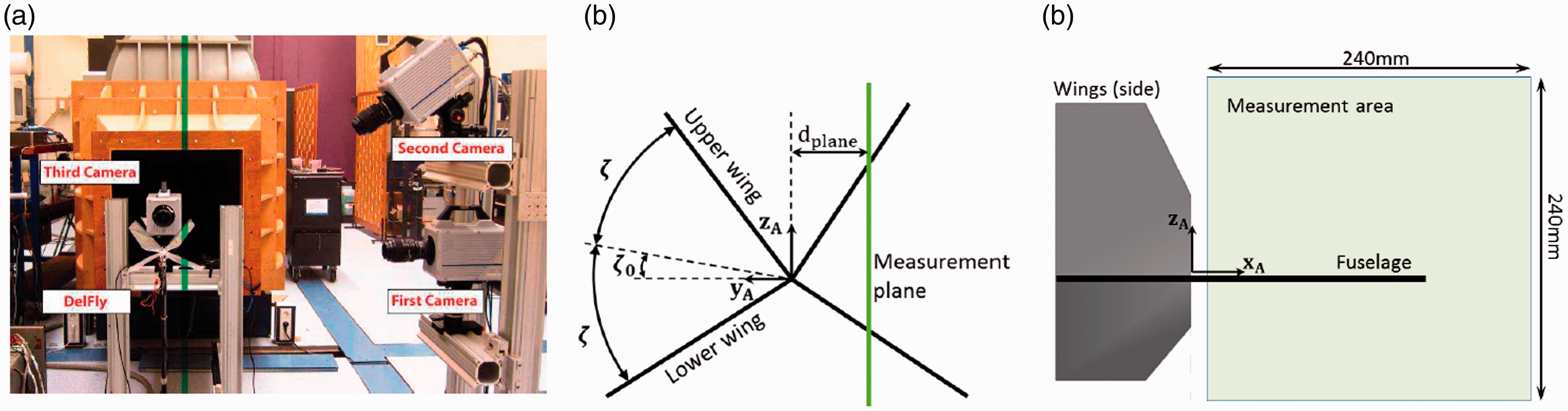
Experimental setup for PIV measurements; figures adapted from Perçin. ³¹ (a) Photograph of the setup. (b) Front view (looking at the vehicle). (c) Side view.

Figure 3.

Top view on the FWMAV, showing the main tail geometric features and position, and the area covered by the wake model, in relation to the original region covered by the PIV measurements (measurements in mm).

Data were obtained at 10 different spanwise positions (d_plane) to the right hand side of the fuselage, covering a range from 20 to 200 mm, in steps of 20 mm. At each spanwise position, measurements were conducted in a 240 mm × 240 mm chordwise oriented plane (aligned with the vehicle’s XZ plane), positioned 10 mm downstream of the wing trailing edges, as clarified by Figures 2(b, c) and 3. The planes were each centred around an axis 24 mm above the fuselage, in order to capture the full wing stroke amplitude, considering the 13° wing dihedral of the platform. Double-frame images were captured at a recording rate of 200 Hz, and approximately 30–36 flap cycles (depending on the flapping frequency) were captured at each position. The post-measurement vector calculation ³¹ resulted in a spacing between measurement points of approximately 3.6 mm in each direction. Measurements in the region closest to the wings were found to be unreliable due to laser reflection, hence data acquired in the 60 mm of the measurement plane closest to the wings were discarded. Details on the PIV measurements, experimental setup and pre and post-processing can be found in Perçin. ³¹

Modelling approach overview

We begin by considering a simplified 2D aerodynamic model, where the tail lift and drag forces are assumed to be described by the standard equations

$$L_t=\frac{1}{2}\rho S_t{V}_t^2{C}_{L,t}\left({\alpha }_t\right)$$

(1)

$$D_t=\frac{1}{2}\rho S_t{V}_t^2{C}_{D,t}\left({\alpha }_t\right)$$

(2)

where ρ is the air density, S_t is the tail reference area, V_t is the flow velocity, α_t is the angle of attack (AOA) of the tail, and C_Lt and C_Dt are the lift and drag coefficients of the tail, respectively, as a function of tail AOA.

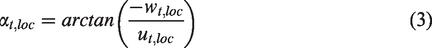
The AOA and velocity experienced by the tail are significantly affected by the downwash from the flapping wings. As a consequence, they are time-varying and complex, and depend on both the wing kinematics and the free-stream conditions. Additionally, the velocity and AOA perceived by the tail vary depending on the spanwise location that is considered. In view of the spanwise changes, a blade element modelling approach was opted for, using differential formulations of equations (1) and (2) (cf. equations (20) and (21)). This implies that 3D effects are neglected, as discussed subsequently in ‘Assumptions’ section. While quasi-steady blade-element modelling is a significantly simplified formulation, its use is widespread in the flapping-wing literature, where it has frequently been found to yield somewhat accurate approximations of unsteady flapping-wing aerodynamics.^12,32–34 This type of formulation was therefore considered acceptable to approximate the aerodynamics of the tail, which can be seen as a flat plate in a time-varying flow.

According to blade-element theory, the local AOA and velocity experienced at each blade element can be expressed as follows

$${\alpha }_{t,\mathit{loc}}=\mathit{arctan}\left(\frac{-w_{t,\mathit{loc}}}{u_{t,\mathit{loc}}}\right)$$

(3)

$$V_{t,\mathit{loc}}=\sqrt{u_{t,\mathit{loc}}^2+w_{t,\mathit{loc}}^2}$$

(4)

where u and w are, respectively, the x and z components of the local velocity perceived by the tail blade element, according to the coordinate frame defined in Figure 2. Each component includes the contribution of the free-stream velocity ( $V_{\infty }$ ), as well as the contribution of the wing flapping-induced velocity at the spanwise position considered, as explained in ‘Effective velocity and AOA on the tail’ section (cf. equation (6.1)). Figure 4 illustrates the different flow velocities acting on a tail section (blade element), as a clarification, as well as the resulting flow velocity vector $V_{t,\mathit{loc}}$ , given by the combination of free-stream and wing-induced velocities. Note that the tailplane has approximately no constructive incidence angle, as it is aligned with the xy-plane of the body (as defined in Figure 3).

Figure 4.

Flow velocities experienced at a spanwise tail section (not to scale). α_b indicates the AOA of the vehicle and $V_{\infty }$ is the free-stream velocity (which approximately corresponds to the forward velocity of the vehicle). The wing-induced velocity experienced at the tail section is given by the vector V_i, while the total velocity experienced locally at the tail section is represented by the vector $V_{t,\mathit{loc}}$ , obtained by summing V_i and $V_{\infty }$ . The components of each velocity vector along the x_A and z_A axes, respectively, are shown in grey. On the left, the definition of a blade element with respect to the whole tail is clarified. (a) Tail section (blade element) definition. (b) Local velocities and angles at 2D section (blade element).

Since the free-stream contribution can be approximately computed from the flight conditions, the main unknown is the contribution of the wings. A realistic model of the aerodynamics of a tail positioned behind flapping wings requires representing the time-varying velocity profile that results from the unsteady wing aerodynamics. As a result, the first step in the modelling process is to represent the flapping-wing wake and deduce the resulting effective velocity and AOA on the tail. The second step is, then, to include the induced velocity predicted by the aforementioned model in the differential form of equations (1) and (2). Additionally, there may be further effects that result specifically from the interaction of the free-stream and wake components: these require experimental data to be quantified, and are excluded at this stage.

The overall modelling approach is clarified by the diagram in Figure 5. Throughout the remainder of this paper, this diagram will serve as a reference. The modelling process comprises the following main steps, numbered so as to correspond to the numbers shown in the figure:

The necessary data must be obtained, i.e. the input to the model. The geometry and position of the tail are known for a given vehicle. The flight condition (velocity, wing flap phase and wing flapping frequency) can be determined through flight testing, if a flight-capable vehicle is already available, or otherwise based on similar vehicles. If online application of the model is desired, the flight condition must be determined in flight.

The induced velocity components, arising from the placement of the tail in the wake of the flapping wings, must be computed. The wake modelling is presented in detail in fourth and fifth sections, and yields the time-varying wing-induced velocity within a comprehensive area behind the wings. The induced velocity is expressed in components aligned with the x_A-axis (u_i) and with the z_A-axis (w_i), respectively, according to the coordinate system shown in Figure 3.

From the wing-induced velocities (u_i, w_i) and the known free-flight conditions ( $V_{\infty }$ ), the resulting flow conditions at the tail ( $V_t,{\alpha }_t$ ) are computed, as explained in ‘Effective velocity and AOA on the tail’, ‘Aerodynamic coefficients’ and ‘Local flow and tail force prediction’ sections. Additionally, the aerodynamic force coefficients of the tail ( $C_{L,t},C_{D,t}$ ) are estimated, as explained in ‘Aerodynamic coefficients’ section.

The final result of the modelling process is given by the tail aerodynamic forces (X_t, Z_t), discussed in ‘Local flow and tail force prediction’ section.

Figure 5.

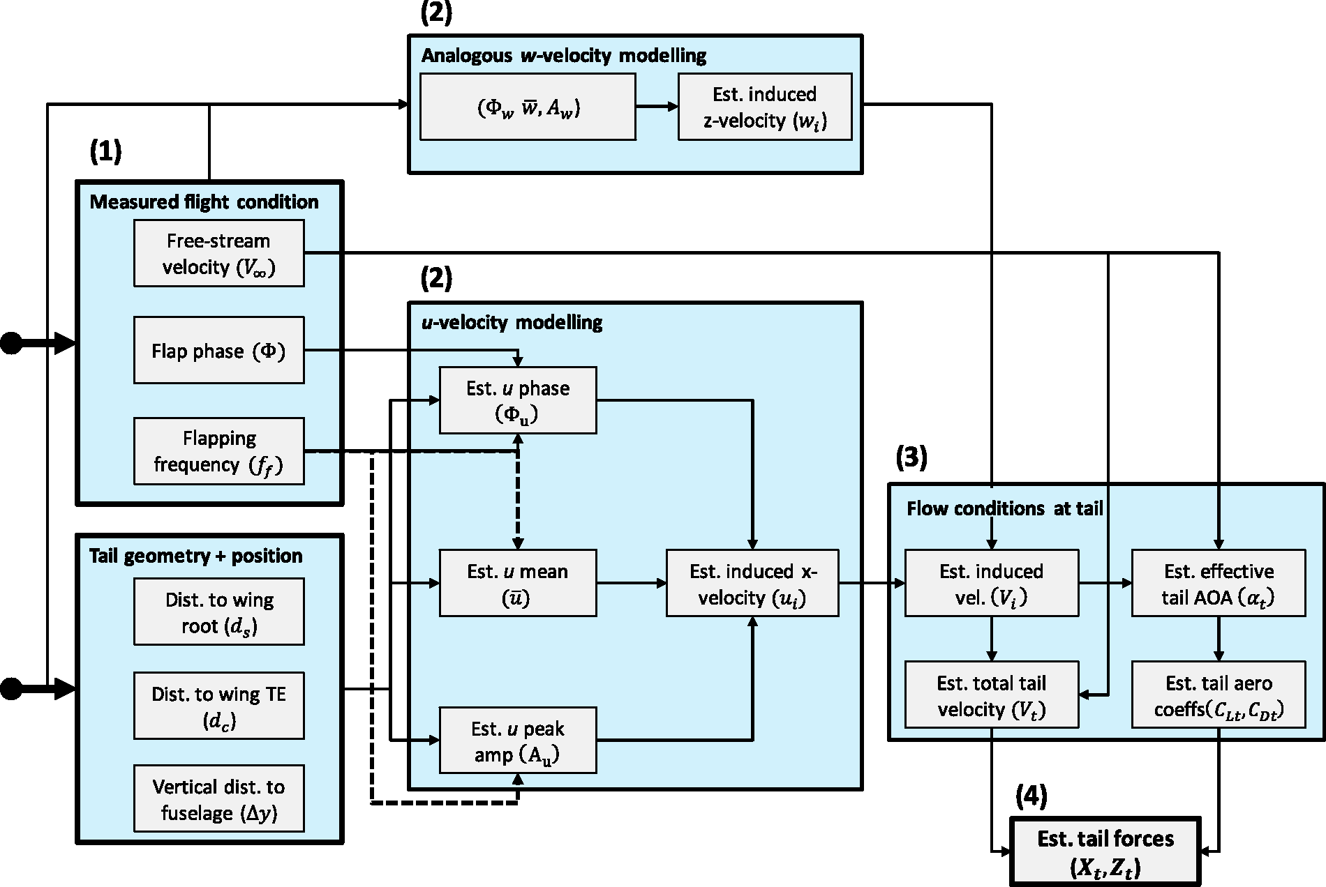
Diagram illustrating the overall modelling approach developed (est.: estimated).

The detailed modelling process is presented and discussed in the following sections.

Wing wake modelling

Experimental evaluation of the wing wake

The velocity experienced by the tail in flapping-wing vehicles consists of a combination of free-stream velocity and induced velocity from the wings, where the latter component imparts a time-varying behaviour to the tail. It is of particular interest here because at the typical flight velocities of the FWMAV considered (0–1 m/s), the induced velocity was found to be of a comparable order of magnitude to the free-stream velocity. Prior to modelling, the PIV data were analysed to establish the main trends and derive a suitable modelling approach.

Whilst initially all available measurements were considered, finally the focus was placed on those relevant for the current tail configuration and possible variations from it – i.e. data collected within a small area around the present tail configuration, as shown in Figure 3. Therefore, only these data were used to model the wake. In spanwise (y_A in Figure 2, or y_B in Figure 3) direction, data collected at distances up to 85 mm from the fuselage impinge upon the current tail design. As larger spans are being considered for future designs, data up to 100 mm from the wing root were considered. Based on analogous considerations, in x_A (or x_B) direction, the domain of interest was reduced to the first 150 mm behind the wing trailing edges.

In z_B direction, data for a small range of values above and below the fuselage were evaluated, to gain an idea of the variation of the flow in this direction (cf. Figure 6). Although the tail essentially remains within approximately the same plane, it was considered useful to consider such changes because the tail has a thickness, and its position may vary slightly with respect to the static case due to vibrations and bending of the fuselage during flight.

Figure 6.

Velocity component u (mean and peak amplitude) obtained at different spanwise and chordwise positions, for four different vertical positions (z), at 11.2 Hz flapping frequency. (a) Mean of u. (b) Peak amplitude of u.

Short samples (3s) of the velocities in x_A and z_A direction (i.e. u and w, respectively) measured at each chordwise (d_c) and spanwise (d_s) position considered in the subsequent modelling process (cf. ‘Sinusoidal model structure of the wing wake’ section) are shown in Figure 7. The definition of the wake positions with respect to the wings is clarified in Figure 3. The data in Figure 7 are discussed further in the remainder of this section. Additionally, an overlap of velocity measurements obtained at different chordwise distances from the wings and constant spanwise position is shown in Figure 8 – here a qualitative idea can be obtained of the periodicity of the wake, and of the gradually increasing phase lag at increasing distances from the wing trailing edges. An initial assessment of the data allowed for the following three main observations.

Figure 7.

Measured wake u and w flow velocities at different chordwise (d_c) and spanwise (d_s) distances (data from Perçin ³¹ ).

Figure 8.

Overlapped measurements for velocity components u and w obtained at different chordwise positions, at a fixed vertical position (approximately in the plane of the tail), for a spanwise position $d_s=60\text{mm}$ ; and corresponding angle between upper and lower wings, $2\zeta$ (cf. Figure 2(b)).

Firstly, it was found that the induced velocity in x_A direction (u) is the main contributor to the average wake velocity, while the mean w velocities are much smaller, often close to zero (cf. Figure 7). However, both components show significant oscillations during the wing flap cycle and hence both should be considered in a time-resolved model. The oscillations in w velocity also influence the local AOA on the tail (cf. equation (3)).

Secondly, both the time histories (cf. Figures 7 and 8) and the discrete Fourier transforms (DFT) of the measurements reveal that the wake is highly periodic – with the exception of some isolated parts – and at fixed positions in the wake there is considerable agreement between separate flap cycles. This suggests that the velocity variations can be directly related to the wing flapping. Nonetheless, at some positions in the wake, the data become noisier and display more variation between cycles (e.g. at $d_c=80\text{mm},d_s=20-40\text{mm}$ ). This may be due to additional complex interaction between the vortices in the wake, ²¹ but also due to PIV imperfections. In the current study, the wake is assumed to be periodic (cf. ‘Assumptions’ section). This captures the main effects observed, while yielding less complex and more interpretable results.

Thirdly, it was found that in most of the domain relevant for the tail, the frequency content is largely concentrated at and around the flapping frequency (cf. Figure 9). Thus it was considered acceptable, for a first approximation of the velocities on the tail, to low-pass filter the data just above the flapping frequency. Nonetheless, there are isolated parts of the wake where this assumption becomes questionable, e.g., very close to both the wing trailing edges and the wing root. These are the same locations mentioned in the previous point. At these locations, it was also found that the frequency content shifts towards higher harmonics. This cannot be captured by the current model, but will be considered in future work.

Figure 9.

Example of the effect of low-pass filtering just above the flapping frequency ( $\sim 12\text{Hz}$ ), in the time and frequency domain (wake position shown: $d_s=20\text{mm},d_c=90\text{mm}$ ; DFT frequency resolution: 1.2 Hz). (a) u, time domain. (b) u, frequency domain. (c) w, time domain. (d) w, frequency domain.

As the velocities are mostly periodic, the amplitude and phase of the oscillations were considered next. Figures 7 and 10 show that there are trends in the peak amplitude and phase of the wake velocity, with both the chordwise distance (d_c) from the wing trailing edges, and the spanwise distance (d_s) from the fuselage. The measurements obtained very close to both the wing root and the wing trailing edge are often less clean than those obtained elsewhere, possibly due to the complex aerodynamics resulting from the vicinity of the upper and lower wings to each other and their mutual interference. It is also possible that some of these effects are due to the wake not yet being fully developed very close to the wings. Similarly, the data obtained directly behind the wing tips are noisy and only barely periodic, possibly due to wake contraction, ³⁵ which implies that at increasing distances behind the flapping wings, the wing wake occupies an area that is increasingly narrower than the wing span, so that at some distance behind the wing tips, the wing wake has only a negligible effect. However, for the current FWMAV it is unlikely that even new tail designs would become as wide as the wings. Due to the described effects, the clearest measurements were obtained at intermediate spanwise distances (d_s), away from both the wing root and the wing tip, with some exceptions due to unsteady effects mentioned in the previous paragraphs. It is interesting to note that generally the mean u velocities initially increase, but then decrease with spanwise distance. This may be related to the specific vortex formations, but may also be enhanced by the dihedral of the wings. As the tail is aligned with the fuselage, at increasing spanwise distances from the wing root, the tail plane is increasingly less influenced by the main vortex formations.

Figure 10.

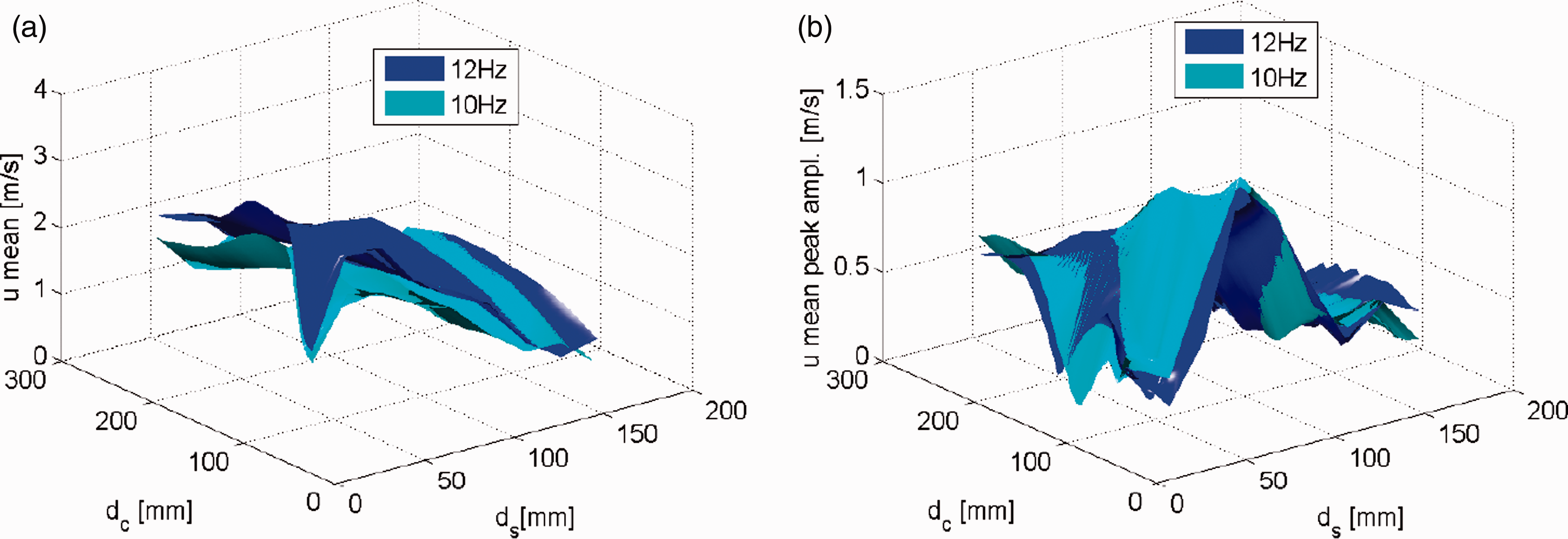
Velocity component u (mean and mean peak amplitude) obtained at different spanwise and chordwise positions and fixed vertical position, for two different flapping frequencies. (a) Mean of u. (b) Peak amplitude of u.

In chordwise direction (d_c), the mean u values generally decrease farther away from the wing trailing edges, with the extent of this decrease varying depending on the spanwise position (d_s), while the w average velocities remain close to zero and show less clear trends. At large distances from the trailing edges, the peaks are small and tend to merge together, which complicates the recognition of patterns. This effect is further enhanced by the PIV settings, typically chosen so as to capture the highest velocity in the measurement plane effectively, to the detriment of lower velocities occurring simultaneously at other locations. In vertical (z_B) direction, changes were found to be small but noticeable in the mean u values, but only minor in the u peak amplitudes (cf. Figure 6) and w velocities.

Comparing the data obtained at the two different flapping frequencies suggests that a higher flapping frequency leads to a higher mean velocity (mainly u), while not significantly affecting the peak amplitudes in the time-varying component. However, the availability of data for only two different flapping frequencies was considered insufficient for reliable conclusions to be drawn, hence this likely dependency was not further considered in the modelling process, at this stage. Contrasting the PIV measurements for different flapping frequencies also reveals similar overall trends, suggesting a degree of reliability. In general, it should be considered that while a full aerodynamic interpretation requires extensive 3D data and analysis beyond the scope of this study, the unsteady processes involved imply that the observed trends may not always be intuitive. In this sense, the aforementioned similarity is a particularly useful indication.

The wing wake modelling approach was based on the preceding discussion and is outlined in the following section.

Assumptions

The following assumptions and simplifications were made within the modelling process.

Based on the discussion in the previous section, the wing wake was assumed to be periodic. As mentioned previously, this is not always the case, nonetheless, even where there are additional effects, the periodic component remains significant, and is dominant in most cases, such that this assumption was considered acceptable for a first approximation. Periodic formulations have also been found to approximate flapping-wing forces with accuracy,^18,36 and hence can also be considered a plausible approach to represent the wing wake.

Based on the frequency content analysis of the PIV data, it was decided to filter the wake velocities just above the first flapping harmonic.

The wing beat was assumed to be sinusoidal. While in the considered FWMAV the outstroke is slightly slower than the instroke, ¹² this difference is small and was considered negligible, ¹² particularly in view of the simplified nature of the aerodynamic model itself. More accurate mathematical representations of the kinematics, e.g., using a split-cycle piecewise representation, ³⁷ or different functions such as the hyperbolic tangent would have increased the model complexity and interpretability, and are left for future work.

Velocities in y_B (or y_A) direction were assumed to be negligible. While these velocities are of comparable magnitude to those in z_B direction, the blade element formulation adopted assumes that spanwise terms do not generate lift. The contribution of the aforementioned component is also assumed to be minor in a cycle-averaged sense because the platform is symmetrical around the $x_B{z}_B$ plane.

Three-dimensional effects, such as tail tip effects, were considered negligible, based on the results in Perçin et al. ²³ and Perçin ³¹ (cf. Figures 5.3 and 5.4 in Perçin ³¹ ). This assumption may become questionable in rapid manoeuvres, where the sudden change of AOA would induce 3D effects – this situation is not considered in the current formulation. More generally, the effect of the tail on the wing wake was not explicitly considered – this highly complex interaction requires extensive further analysis to be understood and modelled. Conducting PIV measurements on the wings alone, rather than on the full vehicle provides clearer insight into the wing wake propagation, as measuring on the full vehicle entails several additional challenges (discussed subsequently in ‘Aerodynamic coefficients’ and ‘Evaluation of main results’ sections).

It was assumed that the wing wake measured in hover conditions can provide information on the tail forces also for slow forward flight conditions, when combined in a simplified way with the free-stream effect (cf. ‘Tail force modelling’ section). The wake vortices have different intensities and propagation rates depending on the free-stream velocity and flapping frequency, ²³ and the wake model is therefore likely inadequate for fast forward flight conditions. Nonetheless, the approach is deemed suitable to develop a low-order and physically representative model of the wake in slow forward flight regimes, which can be used to evaluate the effect of the wake on the tail and the magnitude of the tail forces. As shown in Table 2, the dynamic similarity parameters for the most commonly flown slow forward flight conditions (V < 0.7 m/s) are comparable to the hover case. A more elaborate wake model could be obtained with an analogous approach as that proposed in this study, starting from PIV data collected in different flight regimes, however the result would be extremely complex and outside of the scope of the current feasibility study.

Based on the above points, the developed model is considered applicable for moderate Reynolds numbers (approximately 1000–20,000), where viscous forces are sufficiently small, and at low forward flight velocities, where the effect of the free stream is limited.

Finally, as a clarification: the wake models developed in this section predict the velocity of the flow, according to the coordinate system A shown in Figures 2(b, c) and 3. The velocity that will be used to determine the tail forces in the subsequent section is the velocity of the respective tail section, according to the coordinate system B shown in Figure 3. As the x and z axes of the two systems are reversed (rotation by π rad about the y axis), the u and w components of the tail velocity have the same sign as the corresponding components of the flow velocity.

Sinusoidal model structure of the wing wake

The two components of the wake velocity (u, w) were approximated as cosine waves

$$\widehat{u}\left(d_s,d_c,\zeta \right)=\overline{u}+A_u\left(d_s,d_c\right)\cos \left({\Phi }_u\left(d_s,d_c,\zeta \right)\right)$$

(5)

$$\widehat{w}\left(d_s,d_c,\zeta \right)=\overline{w}+A_w\left(d_s,d_c\right)\cos \left({\Phi }_w\left(d_s,d_c,\zeta \right)\right)$$

(6)

where d_c is the chordwise distance from the wing trailing edges, d_s is the spanwise distance from the wing root and ζ is the instantaneous wing flap angle. The six unknown parameters in the above model are: the mean velocities ( $\overline{u},\overline{w}$ ), the amplitudes of the oscillatory peaks with respect to the mean (A_u, A_w), and the phases with respect to the wing flap phase ( ${\Phi }_u,{\Phi }_w$ ). Each parameter must be known at any position in the wake, within the range considered (cf. Figure 3).

The phase of the induced velocities, in particular, must also be related to the wing flap phase, so that an accurate time-resolved model is obtained, that can predict the velocities in the wake any moment of the wing flap cycle. As mentioned previously, the wing flapping motion of the test platform is assumed to be sinusoidal. The magnitude of the angle of each wing with respect to the dihedral can thus be written as

$$\zeta :=\overline{\zeta }+A_{\zeta }\cos \left(2\pi t^{*}\right)$$

(7)

where $t^{*}$ is non-dimensional time with respect to the wing flapping. If the beginning of the flap cycle is considered the moment when the wings are open, the phase corresponds to that of a pure cosine wave. The induced velocities are then waves with the same frequency as the wing flap angle, but phase shifted with respect to it. ${\Phi }_u$ and ${\Phi }_w$ in equation (5) can be formulated as

$${\Phi }_{u,w}=\left(2\pi \left(t^{*}+\Delta t_{u,w}{f}_f\right)\right)$$

(8)

where t is dimensional time, f_f is the wing flapping frequency, and $\Delta t$ is the time difference between the start of the cycle (assumed to occur when the wings are open) and the time at which the peak of the considered wake velocity component occurs.

Applying this formulation requires knowing the time within the flap cycle ( $t^{*}$ ). In practice, one possibility to do this is to use a sensor to register when the wings are at a particular position, measure the time with respect to this instant, and reset to zero every time the wings return to this position. If the flapping frequency is known, the non-dimensional time can be calculated, and the above equations can be applied once the time shift $\Delta t$ is determined. An alternative is to find a function relating flap time to wing flap angle, and measuring the flap angle at each instant. As the same angles occur twice per flap cycle, the result is a piecewise function that also depends on the flap rate. Either way, it can be assumed that the time with respect to the wing flapping is known or measurable.

The relation of each of the six parameters in equations (5) and (6) with position in the wake (d_c, d_s) and flap phase was estimated from the PIV data presented in ‘Time-resolved PIV measurements’ section. This is discussed in the subsequent section. It should be noted that the parameters are likely to also depend on the flapping frequency, however this dependence cannot be determined conclusively with the current data, which only cover two different flapping frequencies. At present, results were determined only for the specific flapping frequencies for which data were available. As the procedure is analogous for different flapping frequencies, results are only presented for the 11.2 Hz case.

Model identification and results

Sub-model identification

The unknown parameters ( $\overline{u},A_u,{\Phi }_u,\overline{w},A_w,{\Phi }_w$ ) in equation (5) (hereafter ‘wake parameters’) were determined from the PIV data presented in ‘Time-resolved PIV measurements’ section using an identification method. In particular, a separate sub-model was developed to estimate each of the six original parameters (cf. Figure 5). In an identification context, each of the wake parameters is therefore the output (z) of a separate sub-model. In view of the assumed wake periodicity, rather than using all measurements, the measured output at each wake position and non-dimensional time instant was defined as the mean overall flap cycles recorded at that particular position and time. Data for 10 flap cycles were used to construct these models, to allow for validation of the results with the remaining data. Moreover, as discussed in ‘Experimental evaluation of the wing wake’ section, changes of the velocities in z_A direction are small but visible, and should be included in the model. Thus, instead of using measurements for the single particular z_A position closest to the tail plane, we computed the average of the velocities measured at the two closest measurement points above and below the tail plane. This covers a distance of approximately 8 mm and should improve the reliability of the final force model results. Given the small magnitude and gradualness of the variation observed in this direction (cf. Figure 6), using a larger number of points is not expected to change the results significantly.

As seen in ‘Experimental evaluation of the wing wake’ section, the wake parameters depend nonlinearly on chordwise and spanwise position with respect to the wings, and on the wing flap phase, hence the sub-models must depend on these variables. To obtain low-order models that nonetheless can represent these dependencies accurately, an identification method based on multivariate simplex B-splines was chosen. This allows for accurate global models to be obtained by combining low-order local ones, thus avoiding the typically high model orders required to cover the entire domain of a nonlinear system with a single polynomial model. A thorough explanation of the estimation method can be found in de Visser et al.,^38,39 hence only a concise overview is given here.

Simplex splines are geometric structures minimally spanning a set of n dimensions. Each simplex t_j has its own local barycentric coordinate system, and supports a local polynomial that can be written (in so-called B-form) as

$$p\left(x\right)=\{\begin{array}{ll}{\displaystyle \sum _{\left|\kappa \right|=d}{c}_{\kappa }^{t_j}}{B}_{\kappa }^d(b_{t_j}(x))\hfill & \text{ for }x\in t_j,\hfill \\ 0\hfill & \text{ for }x\notin t_j\hfill \end{array}$$

(9)

where $c_{\kappa }^{t_j}$ are the coefficients of the polynomial, known as B-coefficients, $b_{t_j}$ are the barycentric coordinates of point x with respect to simplex t_j, d is the degree of the polynomial, $\kappa =\left({\kappa }_0,{\kappa }_1,\dots ,{\kappa }_n\right)$ is a multi-index containing all permutations that sum up to d, and $B_{\kappa }^d(b)$ are the local basis functions of the multivariate spline

$$B_{\kappa }^d\left(b\right):=\frac{d!}{\kappa !}{b}^{\kappa },d\ge 0,\kappa \in {\mathbb{N}}^{n+1},b\ge 0$$

(10)

Polynomials of the form given in equation (9) can be used as a model structure for system identification. The underlying idea is that prior to estimation, the identification domain is divided into a net of non-overlapping simplices (triangulation), and a separate local model is identified for each simplex, using the datapoints contained in that simplex. In an identification framework, the basis functions in equation (9) represent the measurements used to model the chosen system output, whereas the B-coefficients are the model parameters to be estimated and locally control the structure of the polynomial.

In this study, an ordinary least squares (OLS) estimator was used, ³⁸ hence, the output equation at each measurement point i is

$$z_i={\displaystyle \sum _{\left|\kappa \right|=d}{c}_{\kappa }^{t_j}}{B}_{\kappa }^d\left(b_{t_j}\left(x_i\right)\right)+{\mathrm{ϵ}}_i,x\in t_j$$

(11)

Written in vector form, this is

$$\mathbf{z}=\mathbf{Bc}+\mathit{ϵ}$$

(12)

The sparse B matrix in the above equation contains the regressor measurements, converted to the barycentric coordinates of the simplex containing them. As each local model is constructed using only the data within a single simplex, the global B-matrix for the full triangulation is a block diagonal matrix constructed from the B-matrices of the J simplices

$${\mathbf{B}}_{\mathit{glob}}=\mathit{diag}\left({\mathbf{B}}_{t1},\dots ,{\mathbf{B}}_{\mathit{tJ}}\right)$$

(13)

Given the B-matrix, an OLS estimator can be defined for the B-coefficients in c

$$\widehat{\mathbf{c}}={\left({\mathbf{B}}^T\mathbf{B}\right)}^{-1}\mathbf{y}$$

(14)

To ensure continuity between the separate models, continuity conditions of the following form can be defined between neighbouring simplices

$$\mathbf{H}·\mathbf{c}=0$$

(15)

where H is the smoothness matrix defining the continuity conditions. The estimator can then be reformulated to include these continuity conditions, e.g., as explained in de Visser et al. ³⁸

The outlined approach was applied to estimate a model for each of the six wake parameters in equation (5), leading to six separate sub-models that are finally combined to estimate the total time-resolved induced velocity components, as shown in Figure 5. The output variable for each sub-model is thus one of the aforementioned parameters. In each case, an appropriate model structure and triangulation of the domain defined by the chordwise (d_c) and spanwise (d_s) positions in the wake were chosen, based on analysis of the input–output data. The chosen modelling setup for each case is shown in Table 1. In all cases, equally shaped and evenly distributed two-dimensional simplices were used. When comparable results were obtainable with different combinations of model order and triangulation density, the solution leading to the lowest model order was favoured, as it leads to a comparatively smaller number of coefficients and is less prone to numerical issues. Zero-order continuity ^a was considered sufficient at this stage, as the intended usage of the model does not require more.

Table 1.

Modelling parameters for each output variable and performance of the resulting model.

Output	Model deg.	Continuity	# Simplices	RMS	$R^2$
y	d		J
$\overline{u}$	2	0	8	0.05 m/s	1.0
Au	4	0	4	0.01 m/s	1.0
${\Phi }_u$	2	0	8	0.002 s	1.0
$\overline{w}$	2	0	8	0.01 m/s	1.0
Aw	2	0	8	0.01 m/s	1.0
${\Phi }_w$	2	0	2	0.003 s	0.98

Note that in the case of the phase, to facilitate the modelling, the time delay was formulated in a continuous way: starting from the time delay of the earliest occurring peak in the wake, other peaks are taken incrementally, going over into successive cycles, rather than restarting at zero when the delay becomes larger than the cycle period. However, in practice it is useful to know where the peaks in the wake are located at a particular moment in the (current) flap cycle, rather than with respect to the same particular flap cycle that may be more than one flapping period away. Thus, in a second moment, when going from the wave parameters to the actual wave, the phase model results were transformed back into the relative frame of a single flap cycle (with flapping period T_cycle), to yield the relative time delay with respect to the most recent peak

$$\Delta t_{\mathit{rel}}=\Delta t_{\mathit{abs}}\mathrm{mod}{T}_{\mathit{cycle}}$$

(16)

Wake modelling results

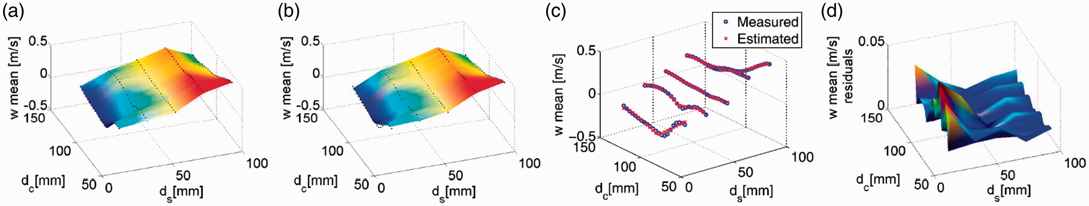
The obtained results are summarised in Figures 11 to 16. It can be seen that in general the respective models represent the PIV-computed wake parameters with significant accuracy, mostly leading to small residuals and high R² values (cf. Table 1 and Figures 11 to 16). The residuals generally tend to be larger close to the wing root, in agreement with the observations made earlier regarding more unsteady regions in the wake, where trends are more nonlinear. Nonetheless, even at these locations, the residuals remain small and the model accuracy high.

Figure 11.

Model: u mean parameter. (a) Measured data surface. (b) Model surface. (c) Measured and model-predicted output. (d) Residual surface.

Figure 12.

Model: u peak amplitude parameter. (a) Measured data surface. (b) Model surface. (c) Measured and model-predicted output. (d) Residual surface.

Figure 13.

Model: u phase delay parameter. (a) Measured data surface. (b) Model surface. (c) Measured and model-predicted output. (d) Residual surface.

Figure 14.

Model: w mean parameter. (a) Measured data surface. (b) Model surface. (c) Measured and model-predicted output. (d) Residual surface.

Figure 15.

Model: w peak amplitude parameter. (a) Measured data surface. (b) Model surface. (c) Measured and model-predicted output. (d) Residual surface.

Figure 16.

Model: w phase delay parameter. (a) Measured data surface. (b) Model surface. (c) Measured and model-predicted output. (d) Residual surface.

Evidently, however, the ultimate goal is to represent the actual wake velocities, and hence to evaluate the extent to which the suggested sinusoidal approximation of equations (5) and (6) is itself acceptable. As observed in ‘Experimental evaluation of the wing wake’ section, the PIV data are predominantly periodic, and in some cases close to a perfect sine wave. Hence, a further evaluation of the obtained wake model was made by substituting the estimated parameters (i.e. the predicted output of the six sub-models) into equation (5) to compute the velocities as each considered position in the wake, and comparing the outcome to the direct PIV measurements. In particular, the PIV data used in this evaluation were not used in the identification process, hence this comparison constitutes an independent validation of the wake model.

Figure 17 shows several examples of the model validation process. It can be observed that, as expected from the PIV data and the highly accurate estimates of the wake parameters, the agreement is generally significant, especially in mean and amplitude, which are mostly very close to those of the data. The amplitude shows some discrepancies, mostly related to the modelling assumption of periodicity, which, as discussed previously, is not always fully valid, rather than to the identified model itself. As discussed in ‘Experimental evaluation of the wing wake’ section, this assumption is particularly questionable close to the wings. The discrepancies in Figure 17 may also have two further sources: (i) the data were collected experimentally, hence were prone to unwanted external effects – small phase shifts in the flapping controller and perturbations in the atmospheric pressure of the test room can affect both phase and amplitude of the flow field; (ii) the PIV data were filtered prior to modelling, which can lead to the exclusion of information with a phase higher that the cut-off frequency (however, higher cut-off frequencies also increasingly cause undesired noise to be included in the model). Point (i) also implies that it can be challenging to distinguish between measurement or experimental setup-related anomalies and real highly unsteady effects in the data – this further motivates the choice of a model capturing only the main effects observed. Overall, the most notable discrepancies are found in the phase, which in some cases is not fully in agreement, as seen in Figure 17 (e.g., at position $d_c=80\text{mm},d_s=60\text{mm}$ ). This may also be a result of insufficient accuracy in determining the flapping frequency, which in some cases varies slightly throughout the data samples. Indeed, it appears that the frequency itself is not always identical, rather than the phase delay. As a small discrepancy in phase may add up to a large error over time, it is especially important that the frequency is determined accurately, and this should be ensured when applying this model. It must be kept in mind that any model represents a simplification, and therefore there is always a reality gap between model and data. The wake model captures 98–100% of the periodic information content in the data (cf. Table 1) and is hence considered sufficiently accurate for the purposes of this study.

Figure 17.

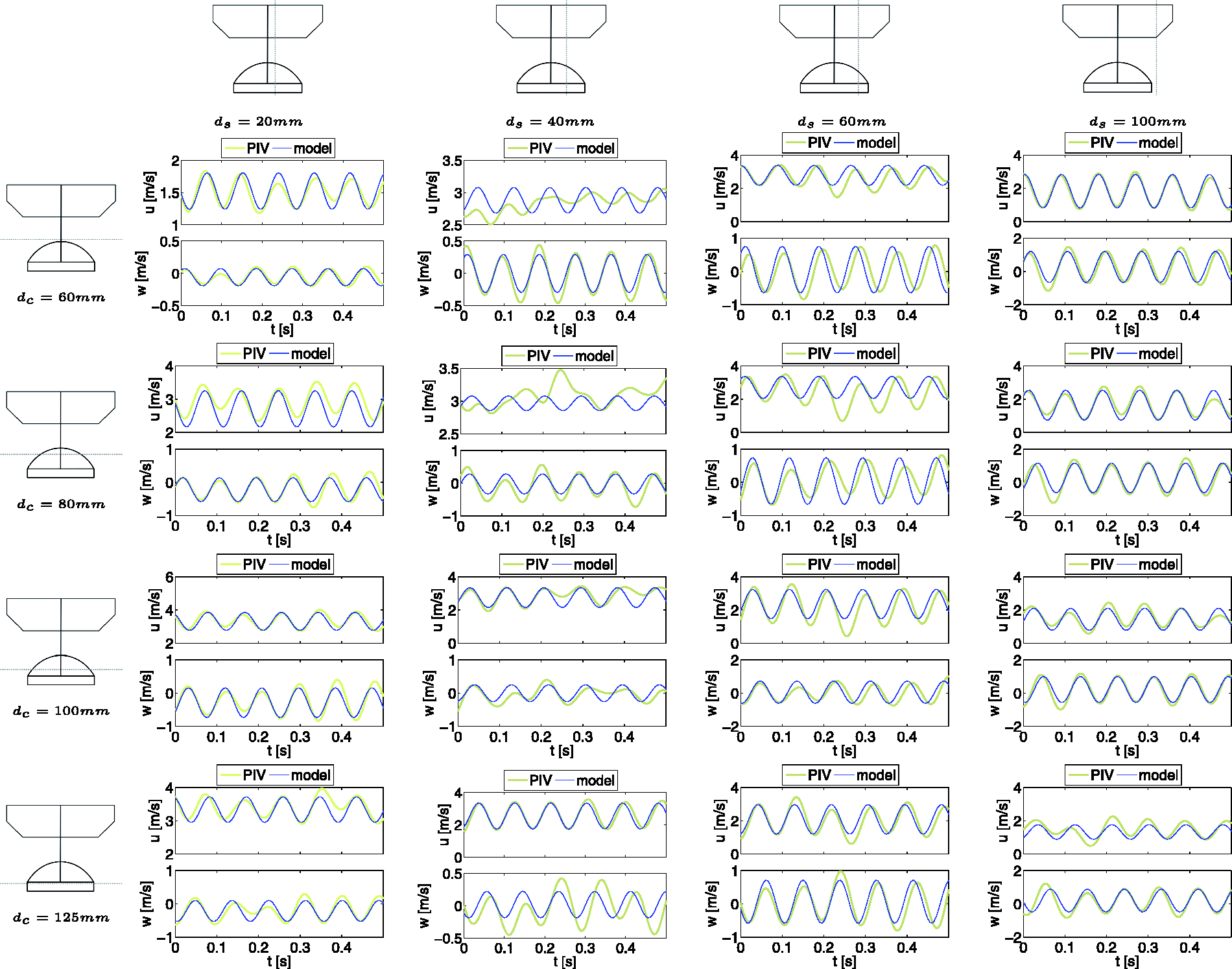
Validation example: model-predicted and measured wake velocities u and w at different wake locations, using equation (5) and the parameters estimated with the sub-models presented in ‘Sinusoidal model structure of the wing wake’ section (PIV data from Perçin ³¹ ).

On a final note, it should be considered that although a relatively large number of parameters (B-coefficients of the sub-models) is required to achieve sufficient accuracy over the entire domain considered, the model structure itself is based on low-order components and does not require heavy computations to implement. Additionally, applying the model for tail force estimation requires only knowing the geometry of the vehicle, and very few measurements, viz. flapping frequency and wing flap angle or timing of each cycle. The model also allows for reasonable estimates to be made for in-between positions in the wake, where no direct measurements were available, thus providing more flexibility, for instance facilitating the use of blade element approaches to compute the tail forces. However, as the flapping-wing wake is unsteady, further analysis may be advisable to confirm what occurs at unobserved positions in the wake. With the available data, the current model provides an effective starting point to represent the wake in a realistic but manageable way.

Tail force modelling

Effective velocity and AOA on the tail

The flapping-induced flow velocity models developed in the previous section can be used within a blade element model of the tail aerodynamics. For this it is necessary to determine the specific velocities experienced along the tail leading edge. Figure 3 shows the platform of the test platform tail. The developed wake model allows for the local induced velocities to be determined anywhere along the tail leading edge, as a function of instantaneous flap phase and spanwise and chordwise position of the point considered. The averaging introduced in vertical direction accounts for small variations and inaccuracies in the nominal z_B positioning of the tail. The suggested model provides a continuous mathematical description of the entire wake in the relevant domain, hence it is possible to determine the induced u and w velocities at any point and, consequently, to define blade elements with an arbitrarily close spacing. Figure 4 clarifies the different velocity components acting at each tail section.

Assuming the vehicle is moving with a forward velocity V, hence is affected by a free-stream velocity $V_{\infty }$ , the body-frame u and w velocities experienced by a particular blade element, and resulting total velocity, are given by

$${\widehat{u}}_{t,\mathit{loc}}={\widehat{u}}_i+V_{\infty }\cos {\alpha }_b$$

(17)

$${\widehat{w}}_{t,\mathit{loc}}={\widehat{w}}_i+V_{\infty }\sin {\alpha }_b$$

(18)

$${\widehat{V}}_{t,\mathit{loc}}=\sqrt{{\widehat{u}}_{t,\mathit{loc}}^2+{\widehat{w}}_{t,\mathit{loc}}^2}$$

(19)

where α_b is the body AOA, the subscript i indicates induced velocities, a hat superscript indicates model-estimated values, and variables without superscript are assumed to be known.

The local AOA and velocity experienced at each blade element can then be computed using equation (3), and the lift and drag forces at each blade element can be determined using differential formulations of equations (1) and (2)

$$d{L}_t\left(r,t\right)=\frac{1}{2}\rho c_t\left(r\right){\widehat{V}}_{t,\mathit{loc}}^2\left(r,t\right)C_{L,t}\left({\widehat{\alpha }}_{t,\mathit{loc}}\left(r,t\right)\right)dr$$

(20)

$$d{D}_t\left(r,t\right)=\frac{1}{2}\rho c_t\left(r\right){\widehat{V}}_{t,\mathit{loc}}^2\left(r,t\right)C_{D,t}\left({\widehat{\alpha }}_{t,\mathit{loc}}\left(r,t\right)\right)dr$$

(21)

where r is the spanwise distance from the wing root to the middle of the considered blade element, and $c_t(r)$ is the tail chord at this position. Note that while the variables are expressed as functions of r, to underline that the equation is evaluated at every spanwise blade element, in fact the local velocity and AOA are a function of both the spanwise and the chordwise position of the tail with respect to the wings, as clarified by equations (5) and (6).

Given that each blade element may have a different orientation, due to the temporally and spatially varying flow, the local definition of lift and drag has a different orientation at each station. Hence, in order to integrate the local forces, the differential forces are first transformed to the body coordinate system, based on the local AOA at each blade element. Integrating these components then yields the contribution of the tail to the body-frame X and Z forces.

Note that, as evident from equations (20) and (21), the aerodynamic forces were assumed to depend only on the instantaneous AOA. It is known that when a wing simultaneously translates and rotates about a spanwise axis, the aerodynamic effects acting on it (rotational forces, Wagner effect, added mass, clap-and-peel) are also affected by the wing rotation velocity and, hence, the AOA rate of change. However, calculating rotational circulation is not trivial, due to the lack of physical insight on the phenomenon and the influence of other parameters (Reynolds number and reduced frequency), and wing rotation effects are often studied numerically. ⁴⁰ The explicit inclusion of such phenomena in the proposed model would hence add significant complexity, with no a priori justification for the specific flight regimes studied. Furthermore, as observed in Taha et al. ⁴¹ (Table 1), the dominant component in the force generation process is the leading edge vortex, which is included in the suggested model. In view of these points, the influence of the AOA rate of change was neglected, allowing for a simple, yet physically representative model to be developed.

Aerodynamic coefficients

The remaining unknowns in equations (20) and (21) are the lift and drag coefficients. Several options can be considered for these parameters, starting from a simple linear theory approach, where $C_{L,t}=2\pi {\alpha }_{t,\mathit{loc}}$ and $C_{D,t}=C_{D0}+k{C}_{\mathit{Di}}^2$ . However, it was considered a more realistic alternative to assume that, as the tail experiences a time-varying flow, its lift and drag coefficients take one of the harmonic formulations typically assumed for flapping wings (e.g. cf. Sane and Dickinson, ⁹ Taha et al., ⁴¹ Wang, ⁴² Dickinson et al. ⁴³ ), and in particular, that stall is delayed due to the unsteady flow on the tail.

Evidently, the most realistic approach to determine the aforementioned coefficients is an experimental approach, however this was found to pose a challenge. On the one hand, flapping-wing vehicles are typically very small, so their tails generate very small forces that may be difficult to measure even with highly accurate force sensors. ⁴⁴ This makes it particularly difficult to carry out measurements on the tail alone. On the other hand, clamping the full FWMAV in the wind tunnel results in vibrations, especially in z_B direction, that are not observed in free flight ⁴⁵ – a significant problem because this is the direction the tail is expected to contribute to most. An additional problem encountered during preliminary wind tunnel tests with the full vehicle was the interference of the strut on which the vehicle is clamped: while this is typically not an issue, the normal flight attitude of the FWMAV used in this study – like that of many insects in slow or hovering flight – involves a high body pitch attitude, which leads to the entire tail being positioned behind the aforementioned strut. Moreover, the strut is shaped in an aerodynamically favourable way, minimising its impact on the flow, only in its uppermost part. The normal flight attitude of the studied test platform leads to the tail being positioned further down, where the strut affects the flow on the tail. Free-flight measurements cannot be conducted on the tail alone or on the vehicle with and without tail, as the vehicle is unstable without a tail. Furthermore, free-flight measurements are more affected by noise and forces cannot be measured directly.^45,46

Obtaining realistic data, that would allow for both the aerodynamic coefficients, and the estimated forces themselves to be validated, would ideally require free-flight force measurements on the tail alone. A possible approach to obtain validation data could be to produce a time-varying flow on the tail by artificial means, without using the flapping wings. This would eliminate the problem of flapping-induced tethering-related oscillations, however it would be challenging to use the obtained data for validation as they would be obtained from a different setup and the shape of the wake is highly sensitive to small changes. Furthermore, the oscillatory flow would introduce considerable noise in the measurements, and considering the small magnitude of the forces on the tail, obtaining reliable validation data would still be challenging. Additionally, free-flight PIV measurements (a technique that has recently been demonstrated for the first time, ⁴⁷ but only for measurements at a distance behind the test vehicle) would allow for more realistic evaluation of the interaction between wake and free stream, without the interference of tethering effects. This could give more realistic insight into the wing wake and wake tail interference, providing further validation of the flow velocity approximation, however it does not provide information on the forces and furthermore requires high-precision control.

Typically, the formulations proposed in the literature specifically for flapping wings and for flat plates performing analogous motions, are empirical and contain vehicle-specific parameters that must be determined experimentally or somehow estimated.^41–43 Given the aforementioned experimental challenges, experimental values from the flapping-wing literature were selected to represent the aerodynamic coefficients, allowing for an approximate, qualitative evaluation of the modelling approach to be made. In particular, we opted to use the coefficients measured by Dickinson and Götz ⁴⁸ in their experimental study on translating model wings. These data were considered a realistic starting point because: (i) end plates were used to reduce 3D effects, hence the obtained coefficients are applicable to wing sections, allowing for a blade element approach such as that proposed in the current study; and (ii) the model wings and experimental setup used can be considered reasonably comparable to the tail studied here, i.e. involving non-rotating, rigid, flat-plate wings, translating at low Reynolds numbers. Nonetheless, it should be considered that the Reynolds numbers occurring at the tailplane (taking an average over the span and over the flap cycle, $R{e}_t\hspace{0.17em}\approx \hspace{0.17em}8000–10,000$ for $V_{\infty }=0.3–1.0\text{\hspace{0.17em}m/s}$ ) are higher than those in the aforementioned study, and therefore the coefficients only allow for an approximation. Accurate results will require refining these values based on experimental measurements on the specific test platform, although studies have suggested that differences in coefficients are limited for $\mathit{Re}\hspace{0.17em}\approx \hspace{0.17em}{10}^2–0^5$ , ⁴⁹ and the result obtained with the current coefficients may therefore also provide some quantitative information.

Empirical functions were fitted through the measurements in Dickinson and Götz ⁴⁸ (cf. Figure 4 in Dickinson and Götz ⁴⁸ ). In particular, the following functions were found to yield an accurate approximation, as shown in Figure 18

$$C_{L,t}=C_l\sin 2{\alpha }_{t,\mathit{loc}}$$

(22)

$$C_{D,t}=C_{d0}{\cos }^2{\alpha }_{t,\mathit{loc}}+C_{d\frac{\pi }{2}}{\sin }^2{\alpha }_{t,\mathit{loc}}$$

(23)

where C_l, $C_{d0}$ and $C_{d\frac{\pi }{2}}$ are constants, which were set to the following values, obtained via least squares regression: $C_l=1.6,C_{d0}=0.2,C_{d\frac{\pi }{2}}=2.8$ . It is worth noting that functions of the same form have been used previously to model the aerodynamic coefficients of flapping wings or plates, however these were derived from measurements performed on finite-span, rotating plates/wings. ¹⁰

Table 2.

Flight conditions the tail force model was tested for, corresponding to conditions determined in free-flight tests on the same vehicle; ⁴⁶ and corresponding Reynolds numbers (Re) and reduced frequencies k ( $k=\frac{\omega \overline{c}}{2V_{\mathit{ref}}}$ ).

Test condition	$V_{\infty }(\text{m/s})$	${\alpha }_b(\text{deg})$	$f_f(\text{Hz})$	Re	k
PIV 1	0	N/A	9.3	10,000	0.28
PIV 2	0	N/A	11.3	12,100	0.28
1	0.3	83	13.3	14,500	0.28
2	0.5	74	12.5	14,100	0.27
3	0.7	62	11.7	14,200	0.25
4	1.0	45	10.3	14,700	0.21

The PIV measurement conditions are also shown – these represent the pure hover case and do not directly correspond to free-flight conditions, hence the corresponding body AOA α_b is not known.

Figure 18.

Empirical functions representing the aerodynamic coefficients obtained experimentally in Dickinson and Götz, ⁴⁸ used in this study.

A full validation will involve adjusting the aerodynamic coefficients to the specific test platform, which in turn will require more extensive wind tunnel testing, with a considerably more elaborate setup, and will be considered in future work. Despite the limitations mentioned, the aerodynamic coefficients from the literature provide the means for an initial computation of the tail forces, which in turn yields more insight on the role of the tail.

Local flow and tail force prediction

Results were computed in four different forward flight conditions, chosen to correspond to conditions previously measured in free flight with the same vehicle, ⁴⁶ and shown in Table 2. The properties of the PIV test conditions are also shown. The flight conditions are defined with respect to the full vehicle. Note that the reduced frequency is calculated considering a mean tail chord of 78 mm and a reference velocity that includes the contribution of both the free stream and the wing velocity due to flapping.

Prior to discussing the forces, it is interesting to consider the effective AOA and velocity resulting at the tail from the suggested modelling approach, and the variation of these values both within the flap cycle and along the tail span. The flow conditions depend solely on the proposed wake model and are not affected by the assumptions on the aerodynamic coefficients. It can be observed that the local AOA at the tail is lowered significantly by the velocity induced by the flapping wings, which leads to values within the typical linear regime of a flat plate for a significant part of the tail ( $d_s\hspace{0.17em}\approx \hspace{0.17em}20-70\text{mm}$ ), as highlighted in Figures 19(a) and 20(a). This may help to explain why the tail still generates forces at AOAs that are clearly outside the range that leads to force generation on a flat plate, even though presumably a significant part of the forces is also caused by unsteady mechanisms. Additionally, this suggests that the simplified lift and drag formulations (equations (1) and (2)) chosen may indeed be acceptable for a first approximation, despite being unable to capture all effects.

Figure 19.

Local flow conditions and Z-force on the tail at each section along the leading edge, for $V_{\infty }=0.5\text{m/s}$ . Note that the velocity and AOA are instantaneous variables, which take on a specific value at every spanwise position, but the resulting force is an integral along the span, hence the force at each spanwise position depends on the – in practice finite – blade element size. This explains the different subplot representations.(a) Local cycle-averaged AOA and velocity along tail leading edge. (b) Local cycle-averaged Z-force at each tail blade element.

Figure 20.

Local lift coefficient and AOA at different positions along the tail, for different free-stream velocities. (a) Local angle of attack. (b) Local lift coefficient.

Figure 19(a) shows that the cycle-averaged local velocity at the tail first increases, reaching a maximum between approximately 40 and 60 mm from the wing root (corresponding to $\sim 50-70\%$ of the tail span) and then decreases again outwards along the tail leading edge towards the tip of the tail (cf. Figure 20(a)). This behaviour is in agreement with experimental studies on birds, ²⁸ and has a considerable impact on the force production. It is therefore useful for design purposes, and may help to explain the large differences observed between short and long tails of similar area or aspect ratio. ⁴⁴ The effective cycle-averaged AOA behaves in a complementary way, first decreasing and then increasing. This is consistent with the variation in flapping-induced velocity: where there is less induced velocity, the AOA is closer to the AOA of the wings/body and the contribution of the free stream becomes relatively more important compared to that of the flapping. The trends also agree somewhat with experimental measurements conducted in the near wake of bats. ²⁸

The spanwise variation is interesting in terms of design, because it already suggests that in the current FWMAV design the central-outer part of the tail is more critical for force production. This for instance would imply that increasing the span is highly effective up to a certain point, and then rapidly decreases in effectiveness, presumably because at this point the outer part of the tail falls outside the principal flapping wing-induced velocity region. In turn, this may be helpful when designing the shape of a new tail and deciding how to distribute the surface area. While the induced velocity is not the only important factor to consider, it does provide important hints. Note that the region of highest effectiveness depends on the specific design considered, as it is influenced not only by the wing wake itself but also by the geometry and position of the tail.

At time-resolved level, a gradual phase advance can be observed in Figure 20(a), with movement towards the tip. Moreover, the oscillatory component increases in the same direction (i.e. larger peaks), echoing the increased peaks particularly in w-velocity along the same direction (e.g., cf. Figure 7).

With increasing forward velocity of the body, the general trends remain similar, however the peaks and troughs move closer together, leading to less variation in the time-varying component. This may be due to the smaller contribution of the free-stream velocity to the w-component at higher velocities. The mean local AOA increases at higher free-stream velocities, but not to a significant extent. While at higher forward velocities the flapping-induced velocity becomes less important compared to the free-stream velocity, hence the mean local AOA should be closer to that of the body, at the same time the body is at a lower pitch attitude to begin with, so the overall effect is partly cancelled out. By contrast, at very low forward velocities (cf. Figure 20(a)), some of the local AOA values are even temporarily negative during the flap cycle, which is possible due to the w-component of the induced velocity, which varies in direction, and during the flap cycle can reach a similar magnitude to u.

Initial results for the tail forces were obtained using the proposed aerodynamic coefficient formulations (equations (22) and (23)). Figure 20(b) shows the resulting local lift coefficients at different sections along the tail leading edge. Coefficients are shown for the three different flight conditions shown in Figure 20(a), and presented in a single plot to allow for easier comparing of the impact of the free-stream velocity on the phase and amplitude of the local coefficients. It can be observed that the coefficients largely replicate the trends in the local tail AOA, with the phase advancing and the oscillatory peaks growing in amplitude at further outboard sections. The mean lift coefficients also generally increase with increasing free-stream velocity, and the trend is more evident than in the AOA. It seems that at higher velocities, the effect of the larger free stream experienced by the tail, due to the higher velocity and lower body pitch, dominates over the slight decrease in induced velocity from the wings.

The tail forces predicted by the suggested model are shown in Figure 21, for two wing flap cycles. Given the approximate values chosen for the aerodynamic coefficients, at this stage the results are mainly evaluated qualitatively. As expected, the contribution in x_B direction is minor (approximately 10 times smaller than in z_B direction), and tends to zero particularly at low forward velocities, where it mainly represents parasitic drag and friction. In the case of elevator deflection – in free flight – the X force is expected to increase in magnitude (i.e. become more negative), resulting in an increment in the control moment. The contribution to the Z force is more significant. While the values are small ( $\sim 0.01-0.03N$ ), it should be considered that for the present platform this would constitute up to 20% of the weight force (16 g mass), and hence is not negligible. The signs are negative as expected, given that the tail would mainly produce a force upwards, i.e. in negative z_B direction. With increasing forward flight velocities, the tail produces more force, in an absolute sense, which reflects the free-stream effect. Moving outwards along the tail leading edge, the cycle-averaged tail forces largely echo the trends in the total velocity (cf. Figure 19(a)), i.e. they first increase significantly, peak between 50–70% of the span, then decrease again. The most noticeable difference is that towards the tail tip, the tail force decreases more than would be expected from the induced velocity evolution: this is due to the gradual reduction in surface area towards the tip (cf. Figure 3), which results in less force being generated here. As expected, the large variation in flow conditions along the tail has a considerable impact on the force production, and the observed effect and the modelling of it may be useful for control and design work.

Figure 21.

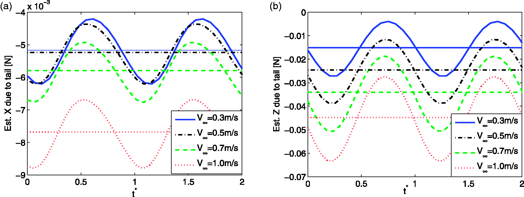
Preliminary tail force results, expressed in body frame, computed using aerodynamic coefficients from the literature. Results are shown for four different free-stream velocities. In addition to the time-resolved forces, the flap cycle-averaged forces are shown as horizontal lines. (a) X-force. (b) Z-force.

While the values of the forces need to be validated using the actual aerodynamic coefficients of the test platform, their order of magnitude is highly plausible (e.g., based on the weight, flight behaviour and wing forces of the vehicle), and remains similar if the aerodynamic coefficients are varied within the range typically encountered in the flapping-wing literature. Additionally, the current model contains a significant amount of information that is based on real data obtained on the test platform, such as the geometry, the test conditions (based on free flight) and, especially, the wake model, which has been validated. Combined, these points suggest that the approach is promising.

On a final note, it should be remarked that the interaction between free stream and wing wake is likely to be more complex than a mere addition, as an increasing free-stream velocity may decrease the vorticity observed in the wake in hover conditions, affecting the wing wake – this will be explored in future work. Nonetheless, the proposed model includes the most significant effects and provides a first approach to formulate predictions characterising and quantifying the role of the tail.

Evaluation of main results

The proposed model represents the time-varying flow and forces on the tail, based on real data, and predicts how these vary, both along the span and within the flap cycle. This, for instance, allows for accurate time-resolved modelling of the forces of the entire vehicle, if the proposed model is combined with a model of the wing aerodynamics. ¹² Additionally, if the model is precise enough and suitable for the considered application, it could provide a basis for (sub-flap) control, for instance, timing the input signals for more effectiveness, or counteracting flapping-induced oscillations.

The model is also potentially useful for tail design studies as it predicts where and when the highest forces can be expected, hence where and when the tail should be most effective. This in turn could be used to shape and position the tail, and possibly the actuators. Finally, the model can be used to predict, approximately, how much effect the tail has on the stability, in terms of how much force it can generate but also more generally if the model is combined with a model of the wing aerodynamics. This would give a more flexible and still physically meaningful overall model, which would for instance be at an advantage compared to black-box models that do not distinguish between the tail and wings.

In particular, the developed model remains directly applicable as long as the wings – and the flow conditions – stay the same, thus it constitutes a helpful tool for comparing different tail designs within a certain design space, once the wing design has been established. This may help to select candidates for the final configuration, or to devise different configurations for different purposes, especially before a flight-capable FWMAV exists. It must be noted that to apply the approach to other platforms (with different wings and/or tails) and varying flight conditions, it is necessary to ensure that the flow conditions and vehicle configuration are comparable to those studied here, and that similar modelling assumptions can be made. Some parts of the high-level approach may be transferable also to more widely differing vehicles, e.g., the wing wake modelling approach. As for any data-driven approach, ideally new measurements are required for an accurate result. Once the required data are available, however, the proposed modelling approach can be easily applied to different (but comparable) vehicles and extended to account for additional effects (e.g., different flapping frequencies).

The proposed model could be improved in accuracy and comprehensiveness by dispensing with some of the assumptions introduced in ‘Assumptions’ section and considering additional effects, e.g., 3D effects. A more thorough investigation of the interaction between wing wake and free stream is particularly advocated. However, obtaining meaningful measurements for such an investigation is challenging (cf. ‘Aerodynamic coefficients’ section). Moreover, while the same modelling methodology can technically be applied to measurements obtained in different flight regimes, constructing a model directly based on all of these data would lead to a significant increase in complexity and consequent decrease in applicability. It would thus be advantageous, prior to extending the model, to investigate how representative the current approach is, through further extensive experimental analysis.

Validation of the aerodynamic coefficients and resulting forces (cf. ‘Aerodynamic coefficients’ and ‘Local flow and tail force prediction’ sections) was found to pose a major challenge, and this represents the main limitation of the current study. As discussed in ‘Aerodynamic coefficients’ section, a complete and realistic quantitative validation of the tail forces will require novel, more advanced experimental techniques, that allow for measurements on the full vehicle (including the wings and tail) in realistic free-flight conditions (e.g., free-flight PIV or novel wind tunnel setups). Future work will therefore focus on investigating such approaches, which would also be highly useful to better evaluate the tail–wake interaction itself. Using CFD approaches for comparison may also provide added confidence in the results, although CFD simulations would not strictly constitute a validation, as they would still require some assumptions to be made, particularly in view of the limited knowledge we have of the FWMAV tail-wing interaction problem. Finally, an improved physical understanding of the flow in the wake may also improve the current results.

While a full validation is outside the scope of this study, due to the many challenges involved (cf. ‘Aerodynamic coefficients’ section), the developed model helps to better understand the role of the tail in FWMAVs, and allows for plausible explanations to be derived for observations made when flying the test vehicle. The model for instance offers an explanation of why the tail can be effective even when vehicle is flying at very high body pitch attitudes, provides an prediction of how much force the tail can produce which qualitatively agrees with the observed flight/control behaviour, and predicts a spatio-temporal distribution of the forces that agrees with studies on biological flyers. These points, together with the modelling approach itself, provide a useful stepping stone for further work on tailed FWMAVs.

Conclusion

This study proposed a modelling approach combining novel multivariate simplex splines and basic quasi-steady aerodynamic theory, to predict the time-resolved aerodynamic forces produced by the tail of a clap-and-peel FWMAV during flight, under the influence of the wing wake. PIV techniques were used to characterise the flow-field in the wake, as a function of spatial position and wing flap phase. After modelling the wake, the model output was validated by comparing the identified model to PIV data not used in the modelling process, revealing significant accuracy. The obtained wake representation was then used to compute the flow conditions at the tail, and the resulting aerodynamic forces acting on the tail, using a standard aerodynamic model and a quasi-steady assumption. The model suggests that the local flow conditions on the tail are significantly altered by the presence of the flapping wings, and are typically pushed closer to the linear steady regime for a significant part of the span, which may help to explain why tails on FWMAVs are so effective. The spanwise evolution of the flow conditions was found to impact the resulting force production significantly. Based on the known mass and flight properties of the test platform, the estimated forces have a plausible order of magnitude when complemented with aerodynamic coefficients from the literature. A full quantitative validation will require further research into new experimental methods allowing for accurate time-resolved force measurements on the full vehicle in realistic free-flight conditions. Future work will hence focus on validating the current results and potentially determining more accurate tail forces, thus closing the research loop. The proposed tail model represents the time-varying flow and forces on the tail based on real data, and thus provides useful insight as well as practical benefits. A combination of the resulting model with a model of the flapping wings has the potential of fully representing the studied vehicle, constituting a useful basis for development of a complete simulation framework, and supporting novel controller development. Furthermore, the developed modelling approach can be a helpful tool for basic design considerations, for instance to predict the effectiveness of a new tail or compare different tails design within the considered design range. The modelling approach can be applied to other comparable vehicles, if wing data are available and sufficient aerodynamic similarity is ensured. Qualitatively, the observations made may also apply to other comparable vehicles, with analogous clap-and-peel mechanism.