Micro air vehicle local pose estimation with a two-dimensional laser scanner: A case study for electric tower inspection

Abstract

Automation of inspection tasks is crucial for the development of the power industry, where micro air vehicles have shown a great potential. Self-localization in this context remains a key issue and is the main subject of this work. This article presents a methodology to obtain complete three-dimensional local pose estimates in electric tower inspection tasks with micro air vehicles, using an on-board sensor set-up consisting of a two-dimensional light detection and ranging, a barometer sensor and an inertial measurement unit. First, we present a method to track the tower’s cross-sections in the laser scans and give insights on how this can be used to model electric towers. Then, we show how the popular iterative closest point algorithm, that is typically limited to indoor navigation, can be adapted to this scenario and propose two different implementations to retrieve pose information. This is complemented with attitude estimates from the inertial measurement unit measurements, based on a gain-scheduled non-linear observer formulation. An altitude observer to compensate for barometer drift is also presented. Finally, we address velocity estimation with views to feedback position control. Validations based on simulations and experimental data are presented.

Introduction

Power utilities, such as transmission line towers, are subject to deterioration due to the atmospheric conditions to which they are exposed. Ensuring their integrity and avoiding network downtime require extensive monitoring programmes. For this purpose, aerial surveys have been increasingly common as they allow covering vast areas in relatively short periods of time, by relying on remote sensing technologies such as thermal imaging, aerial imaging and optical satellites, among others.^1,2 In particular, airborne laser scanning (ALS) technologies have recently attracted a large attention due to their capability of achieving high quality 3D models of infrastructure with high spatial resolution.^2,3 In ALS applications, powerful 3D light detection and ranging (LiDAR) sensors are mounted on manned aircraft, such as helicopters,^1,2,4 then data acquisition is typically carried out using a GPS sensor and an inertial measurement unit (IMU) to keep track of the aircraft’s position and orientation. The geo-referenced range readings are processed afterwards for a wide variety of classification or reconstruction tasks such as detecting power lines,^4,5 vegetation management ³ and making 3D models of the electric towers. ⁶ Nonetheless, the high operational costs of piloted aircraft have constrained the proliferation of these applications. The automation of inspection tasks has thus become a key subject of research in the power industry, in which unmanned air vehicles (UAVs) have surfaced as an attractive solution, as they provide an affordable and flexible means of gathering spatial data.^7–9 This has been mainly fuelled by developments in lithium polymer batteries that have led to larger flight durations and increased payload capabilities. However, these small platforms currently cannot carry the heavy LiDARs required in most ALS applications, and research on inspection tasks with UAVs has mainly focused on vision-based approaches instead.^1,8,10,11 Rapid advances in lightweight LiDARs have made them an appealing alternative for UAVs, and while performance and precision remain far from their 3D counterparts, they can be used for basic and affordable ALS applications, which has already been demonstrated in previous works, for example, for power line monitoring. ¹²

In the context of power utility inspection, GPS sensors remain the predominant choice for achieving autonomous flight capabilities with UAVs. ⁷ Nonetheless, a GPS signal is not always accurate, can be perturbed by the strong electromagnetic fields in the proximity of the power lines ¹³ and provides no perception of the surrounding environment. As a result, a safe collision-free flight cannot be achieved relying on GPS measurements uniquely, which is instead limited to waypoint navigation at large distances from the inspected objects.^1,7,9 On the one hand, vision-based navigation systems have been proposed as a substitute in numerous works, relying mostly on tracking and following the power lines.^10,11 On the other hand, lightweight LiDARs can also be employed for autonomous navigation purposes and have been successfully used for indoor flights with micro air vehicles (MAVs).^14–18 These sensors excel when navigating in cluttered environments, as they directly measure the distance to surrounding objects and naturally open the way for sense-and-avoid functionalities required for safe flights. As a consequence, they can allow achieving higher levels of autonomy and close-up inspections in power line corridors, which is hard to accomplish with other sensors. In this work, we focus on the inspection of transmission line towers, and we explore how 2D LiDARs coupled with commonly available sensors can be used for pose estimation purposes in these scenarios.

Problem statement

One of the first tasks that any autonomous platform must achieve is self-localization. Thus, our primary goal is to obtain real-time estimates of a MAV’s six degree of freedom (DoF) pose with respect to an electric tower, using uniquely on-board sensors and processing capabilities. Our main interest is steel lattice towers made up of rectangular cross-sections commonly used to support high-voltage transmission lines, such as the one shown in Figure 1. For this first case study, we focus on the tower’s body, which makes up the largest portion of the structure. The tower heads have a more complex structure that requires an extensive parameterization^6,19 and are not considered in this work.

Figure 1.

A common high voltage transmission line.

After treating the self-localization problem, the last part of this study focuses on obtaining velocity estimates and sensor fusion techniques are used for this purpose. Accurate velocity estimates are necessary in the control loop to successfully stabilize a MAV’s position. Feedback position control, however, is not addressed in this study. The long-term aim of this work is to achieve autonomous inspection capabilities of electric towers with MAVs.

Related works

While laser range finders have been largely popular among ground robots for autonomous navigation tasks, aerial robots present additional complications that make similar applications not so straightforward. First, flying robots’ motion is 3D. Then, payload limitations prevent the use of more powerful sensors such as 3D laser range finders. Finally, flying robots have fast dynamics that make them harder to stabilize and any state estimation has to be made with low delays and an adequate level of accuracy. This means that estimation and control algorithms must be preferably implemented on board, and must run at high speeds, which limits the complexity of the algorithms that can be used, so as to avoid significant processing delays. Nonetheless, fully autonomous capabilities for MAVs equipped with 2D LiDARs have been shown in numerous previous works,^{14–18,20–23} which have mainly focused on indoors scenarios. Most of these studies adopt a similar strategy: the first goal is to obtain fast and accurate 3D pose estimates from the embarked sensors’ measurements, preferably using on-board processing capabilities; then, a second goal is to derive estimates of the linear velocities using the pose estimates and sensor fusion techniques. We now present how several previous works have addressed these two tasks.

Laser-based local pose estimation on-board MAVs

Regarding the first goal, this is partly achieved by aligning pairs of laser scans to recover the MAV’s relative displacement, a technique known as scan matching or scan registration. While these algorithms can pose a heavy computational burden, satisfying real-time results have been obtained from adaptations of well-known techniques, such as the iterative closest point (ICP) algorithm,^15,17,18,24 and the correlative scan-matching algorithm.^14,16,25 Following the satisfying results previously obtained on-board MAVs, and due to its simplicity and efficiency, the ICP algorithm was chosen for the scan registrations.

Typical approach with the ICP algorithm on-board MAVs

A classic implementation of the ICP algorithm in navigation tasks consists in aligning the current laser scan to the preceding scan. This is known as incremental scan matching and is known to lead to drift over time.^15,17,18 An alternative is to use a keyframe approach, ¹⁷ with a reference scan instead fixed at some initial time. As long as the robot remains in the proximity of this keyframe, and as long as there is sufficient overlap, the estimation error remains bounded and the results are drift free. The ICP implementations proposed in this article go along this line of work.

In general, on MAVs equipped with 2D LiDARs, the ICP algorithm is limited to aligning pairs of 2D laser scans to recover 2D pose estimates. The remaining states are estimated from separate sensing (e.g. IMU for attitude estimation^14–18 and laser altimeter for altitude estimation^14,15). However, to align pairs of 2D laser scans the measurements must be taken within the same plane. This poses a major drawback for aerial robots and requires coping with the 3D motion. A simple solution is to project the laser points to a common horizontal plane using attitude estimations from IMUs.^14,15,18,17 Then, the projected scans are aligned with the ICP algorithm. Nonetheless, this has the underlying assumption that surrounding objects are planar and height invariant, which holds for common indoor scenarios, with mainly straight walls. In an inspection scene, this assumption does not hold as the electric towers have a geometry that varies greatly in 3D. Hence, in our scenario aligning pairs of 2D scans in similar way is not possible. In this work we explore alternative ways in which pose information can be recovered from the laser scans, by exploiting basic knowledge of the tower’s geometry. We also explore two different ways in which the ICP algorithm can be extended to electric tower case.

Limitations of the ICP algorithm for self-localization

It is important to note that scan-matching techniques, such as ICP, only guarantee local convergence and depend highly on a good initial guess.^24,26 A bad initialization may lead ICP to converge to a local minimum far from the optimal solution. Furthermore, these techniques typically cannot recover from large estimation errors. Globally optimal solutions for the ICP algorithm have been studied in the past ²⁷ but are typically too slow for state estimation purposes. In literature, to overcome these issues, it is common for simultaneous localization and mapping (SLAM) techniques to be used in parallel.^14–17,23 These algorithms provide pose estimates with guaranteed global consistency that are less sensitive to initialization errors and that can allow detecting and correcting errors from scan matching. The faster local pose estimates are still required as an odometric input to SLAM, to initialize and speed up the mapping process.^14,17 However, SLAM remains very computationally expensive and is commonly performed off-board,^14,16 with only a handful of studies achieving on-board capabilities,^15,17 at very low rates (2–10 Hz). Thus, the global pose estimates are seldom included directly in the control loop and are mainly limited to providing periodic corrections to the real-time pose estimates from scan matching ¹⁴ and to perform higher level tasks such as path planning^16,17 and obstacle avoidance. ¹⁶ For the purposes of this article, we focus only on the local pose estimation problem, keeping in mind that mapping methods can be used in parallel.

Another complex issue is that scan-matching performance has a strong dependence on the shape of the surrounding environment, as the laser scans must capture sufficient geometric detail in order to extract any useful pose information. The algorithm will thus fail under highly unstructured scenarios, often faced outdoors, or featureless scenarios, such as long hallways or circular rooms. This, in reality, corresponds to inherent limitations of laser range sensing. ¹⁴ Previous works have addressed this issue incorporating multiple sensing modalities, such as GPS sensors, ultrasonic sensors and cameras.^21,22 This, however, goes beyond the scope of this work.

Altitude estimation on-board MAVs

On the one hand, on MAVs equipped with 2D LiDARs, altitude is commonly estimated by placing mirrors to reflect multiple laser rays downwards and directly measuring the distance to the ground assuming that the ground elevation is piecewise constant for the most part.^14,16,17 However, to account for potential discontinuities and changing floor elevations several solutions have been proposed, such as creating multilevel grid maps of the ground ¹⁶ or creating histograms of the range measurements to detect edges and floor level changes. ¹⁷ While this has proven to be effective when navigating indoors, performance remains highly dependent on the floor’s layout, which can be very irregular in typical outdoor inspection scenarios.

On the other hand, barometric sensors are also popular among commercial MAVs. These sensors estimate the absolute or relative height of an object by measuring the atmospheric pressure. However, fluctuations in pressure due to weather conditions cause these height measurements to drift over time. Sensor fusion techniques are thus used to estimate and compensate this drift by using additional sources such as GPS ²⁸ and IMUs.^29,30 More recently, differential barometry has been gaining popularity.^31,32 In this configuration, a second barometer is set stationary on the ground and used as a reference measurement to track changes in local pressure, effectively reducing drift and increasing accuracy.

Attitude estimation on-board MAVs

Fast and accurate attitude estimates are an essential part of any MAV platform. Absolute attitude information can be recovered from magnetometers and accelerometers.^33–35 On the one hand, magnetometers provide measurements of the surrounding magnetic field in the body-attached frame and allow deducing the MAV’s heading.^33,36 However, they are very sensitive to local magnetic fields and measurements can be noisy. On the other hand, accelerometers measure the so-called specific acceleration. When the linear acceleration is small, this sensor directly measures the gravity vector, thus acting as an inclinometer and providing direct observations of the roll and pitch angles. This is a common assumption applied in attitude estimation,^33,35,37 which has shown to work well in practice. On the downside, accelerometers are highly sensitive to vibrations induced by the propellers and require significant filtering to be useful. ³⁴ This in exchange can introduce important latencies in the estimations. Thus, complementary attitude information is commonly obtained from gyroscopes, which measure the angular velocity along the three rotational axes in the body-attached frame. These sensors are less sensitive to vibrations and are very reliable. Absolute attitude can be recovered for the three rotational axes by integrating the measured angular rates; however, this causes the estimation error to grow without bound. ³⁴

Hence, sensor fusion techniques are used to combine the information from all three sensors to tackle drift and noise issues and to obtain more accurate attitude estimates. In literature, the use of linear stochastic filters, such as Kalman filters ³⁴ or extended Kalman filters,^38,39 as the means to fuse inertial measurements is very common. While these filters have been successful in certain applications, they can have an unpredictable behaviour when applied to non-linear systems. ⁴⁰ An alternative is to use non-linear observer design techniques, which present strong robustness properties and guaranteed exponential convergence.^33,40 Numerous recent works have shown successful results in obtaining accurate attitude estimates from noisy and biased measurements using low-cost IMUs.^40,41 In this work we adopt a non-linear observer formulation to obtain attitude estimates.

Velocity estimation on-board MAVs

Literature regarding MAV velocity estimation is very vast and is linked to the type of sensing used on-board. We focus on the approaches applied on MAVs equipped with 2D LiDARs. On one side, directly differentiating the position estimates is avoided as this provides noisy and inaccurate results.^17,18 Instead, sensor fusion techniques are employed to achieve high-quality results by combining laser estimates and inertial measurements. Stochastic filters, such as EKFs, are predominantly used for this purpose,^14,15,20 while simpler complementary filters have also provided satisfying results. ¹⁸ Other works focus on using a cascade of filters for further noise reduction. Dryanovski et al. ¹⁷ first used an alpha–beta filter to obtain rough initial velocity estimates from the laser position estimates, which are then used as a correction in a Kalman filter which includes inertial measurements. Shen et al. ¹⁵ proposed a cascade of two separate EKFs to achieve accurate results and high rates.

Technical background

Sensor set-up

One of the first design challenges with MAVs is choosing the right on-board sensor set-up, which is tailored to the specific task at hand. In this section we present our choice for the sensor set-up.

2D laser rangefinder

Since odometric sensors to measure raw displacements are not available for MAVs, alternative approaches have to be used. In this work we are interested in using laser range measurements from LiDARs for this purpose. However, due to payload limitations only 2D LiDARs can be used,^14,16,17 and complete 3D pose estimates cannot be obtained from the laser range measurements alone. Thus, additional sensing has to be used together with sensor fusion techniques to provide reliable 3D pose estimates.

IMU

At the heart of MAV platforms one commonly finds IMUs comprised of a three-axis accelerometer, a three-axis rate gyroscope and a magnetometer. ³³ In this work magnetometers are not used as they are highly sensitive to magnetic interference and are very unreliable in the proximity of the power lines. We thus only rely on an accelerometer and a gyroscope for inertial measurements.

Altitude sensor

With respect to laser altimeters, barometers allow measuring height without any influence of the ground’s layout and are thus more appropriate for outdoor navigation. We mainly focus on barometers as a source of altitude information. While recent works have obtained impressive results with differential barometry,^31,32 the focus of this work is using on-board sensing only, and differential barometry was not considered.

Experimental set-up

Several experiments were carried out with a quadrotor platform developed at our lab, shown in Figure 2. This MAV was equipped with a Hokuyo URG-30LX 2D laser scanner mounted horizontally on top and providing measurements at 40 Hz. This sensor was connected to an on-board Odroid-XU computer, where all the laser data acquisition was performed. A Quantec Quanton flight controller card based on an STM32 microcontroller was used to estimate the quadrotor’s attitude from measurements obtained from an MPU6000 three-axis accelerometer/gyrometer unit. Lastly, at the time of the acquisitions, the MAV was equipped with an SF10/A laser altimeter from Lightware Optoelectronics, which provides readings at 20 Hz of the distance to the ground along the body-fixed vertical axis. This platform was used towards the beginning of this research to conduct several test flights in front of real electric towers (see Figure 3). The acquired data were then analysed and served as a basis to the methodology developed in this work. While our final results are mostly based on simulations, and focus on using barometer sensors for altitude estimation, interesting experimental results from these initial test flights will be presented where altitude information was obtained from the laser altimeter.

Figure 2.

Quadrotor developed at ISIR, equipped with a Hokuyo URG-30LX 2D LiDAR, an MPU6000 3 axis accelerometer/gyrometer unit and an SF10/A laser altimeter from Lightware Optoelectronics.

Figure 3.

(a) Acquiring laser measurements on an electric tower from a 60 kV distribution line, with the quadrotor from Figure 2 and (b) the equivalent simulation set-up.

Simulation set-up

The approaches proposed in this work were validated in simulations using the Gazebo simulation environment ⁴² and ROS as an interfacing middleware, ⁴³ on a PC with an Intel 3.4 GHz Quad-Core processor and 8 GB of RAM. The Hector quadrotor stack from ROS ⁴⁴ was used to simulate the quadrotor kinematics and dynamics. Regarding the sensors, the simulated IMU published gyrometer and accelerometer readings at 100 Hz, and the barometer sensor provided measurements at 20 Hz. The 2D laser scanner from Gazebo was set to match the characteristics of a Hokuyo URG-30LX sensor: 40 Hz scan frequency, ${0.25}^{°}$ angular resolution and ${270}^{°}$ field of view (thus 1080 measurements per scan). This sensor was mounted horizontally on top of the simulated quadrotor. A CAD model of an electric tower body was used, whose dimensions are $2.5\text{m}\times 3.5\text{m}$ at the ground level and $1.5\text{m}\times 2\text{m}$ at a height of 10 m. These dimensions roughly correspond to those of the tower from Figure 3(a). The complete simulation set-up is shown in Figure 3(b). All algorithm development was done using C++ and the registration and sample consensus modules from the open source Point Cloud Library. ⁴⁵

Notation

Let us denote by $\mathcal{I}$ an inertial North-East-Down frame located at the centre of the tower at the ground level. Let $\mathcal{B}$ denote a body-attached frame in the MAV’s centre of mass. For simplicity, we consider that this frame coincides with the sensor frames. Then, let $\text{ξ}={(x,y,z)}^{\mathrm{⊺}}$ denote the position vector of $\mathcal{B}$ with respect to $\mathcal{I}$ (i.e. the position vector of the MAV’s centre of mass) expressed in $\mathcal{I}$ . Next, R denotes the rotation matrix from $\mathcal{B}$ to $\mathcal{I}$ . Using the Z–X–Y Euler angle convention with roll $\varphi$ , pitch θ and yaw ψ angles, this rotation matrix is expressed as

$$\begin{array}{c}R(\psi ,\varphi ,\theta )=R_z(\psi )R_x(\varphi )R_y(\theta )\\ =\left(\begin{array}{ccc}c\psi c\theta -s\varphi s\psi s\theta & -c\varphi s\psi & c\psi s\theta +c\theta s\varphi s\psi \\ c\theta s\psi +c\psi s\varphi s\theta & c\theta c\psi & s\psi s\theta -c\psi c\theta s\varphi \\ -c\varphi s\theta & s\varphi & c\varphi c\theta \end{array}\right)\end{array}$$

(1)

With this notation, $T_X$ denotes a rigid body transformation parameterized by a vector $X$ , such that

$$T_X(p)=R(\psi ,\varphi ,\theta )p+\text{ξ},p\in {\mathbb{R}}^3$$

(2)

for $X=(x,y,z,\varphi ,\theta ,\psi )$ . This defines the six DoF rigid body transformation from $\mathcal{B}$ to $\mathcal{I}$ that transforms the coordinates of a point from $\mathcal{B}$ to $\mathcal{I}$ .

We now recall the basic translational dynamics of multirotor aircraft with respect to the inertial frame ³³

$$\{\begin{array}{ccc}\dot{\text{ξ}}& =& \text{v}\\ \dot{\text{v}}& =& g{e}_3+\frac{\text{F}}{m}\end{array}$$

(3)

where $v={(v_x,v_y,v_z)}^{\mathrm{⊺}}$ denotes the linear velocity of $\mathcal{B}$ with respect to $\mathcal{I}$ expressed in $\mathcal{I}$ ; g is the gravity constant; $e_3={(0,0,1)}^{\mathrm{⊺}}$ ; m is the MAV’s mass and $F={(F_x,F_y,F_z)}^{\mathrm{⊺}}$ is the coordinate vector of the aerodynamic forces acting on the MAV, expressed in $\mathcal{I}$ . At zero air velocity, these forces are reduced to the thrust force generated by the propellers. Developing equation (3) one obtains

$$\{\begin{array}{c}\dot{x}=v_x\\ \dot{y}=v_y\\ \dot{z}=v_z\\ {\dot{v}}_x=\frac{F_x}{m}\\ {\dot{v}}_y=\frac{F_y}{m}\\ {\dot{v}}_z=g+\frac{F_z}{m}\end{array}$$

(4)

These equations will be used in our observer formulation to fuse the information from the multiple embarked sensors and to recover velocity estimates.

2D local pose estimation

In this section we focus on tracking the cross-sections captured by the individual 2D laser scans, which is analogous to determining the 2D pose of the MAV with respect to the electric tower. Specifically, we explore how basic geometric knowledge of the scene can be exploited for this purpose, without the help of additional sensing. As already mentioned, we focus on the body of electric towers made up of rectangular cross-sections. Measurements taken with a 2D LiDAR on the electric tower from Figure 3(a) are shown in Figure 4, where the portion of the tower can be easily identified. The large open spaces on the surface of the tower allow capturing measurements on all of the tower’s faces (Figure 4(a)). However, due to occlusions, the entire cross-section is not always visible (Figure 4(b) to (d)) and very different scanned structures can be observed. In the worst-case scenario (Figure 4(d)), horizontal bars that are part of the tower’s structure block the lateral and back sides from view and only the front side of the tower is captured in the scans.

Figure 4.

Laser range measurements acquired on the tower from Figure 3(a). In the best case, all sides are visible (a). Occlusions sometimes block the lateral and backsides from view (b)–(d). In the worst case, only the front side is visible (d). This happens when horizontal bars on the tower block the lateral and back sides from view.

Tracking the tower thus requires accounting for the different cases that can be faced. The idea is to gradually extract notable features from the laser scans, using basic geometric assumptions, to determine the position and orientation of the tower. The largest concentration of laser beams fall on the side closest to the MAV, and the line segment formed by these points is the most notable feature in the laser scans. This front line, denoted as ${\mathcal{L}}_{\text{front}}$ , allows recovering essential position and orientation information. The coordinate vectors of the left and right corners of this front line segment, expressed in $\mathcal{B}$ , are denoted as $p_{\text{left}}$ and $p_{\text{right}}$ , respectively. Since ${\mathcal{L}}_{\text{front}}$ remains visible even in the worst-case scenario (Figure 4(d)), tracking this line is at the heart of our proposed approach. Then, as the different sides become visible (Figure 4(a) to (c)), more features are available, such as the sidelines ${\mathcal{L}}_{\text{left}}$ and ${\mathcal{L}}_{\text{right}}$ , which provide complementary orientation information and allow determining the depth (and hence the centre) of the cross-section. The back side of the tower is not explicitly modelled, as it is seldom visible and provides unreliable information. Then, the shape of the contour captured by the laser beams allows establishing a connection between the different features. We consider that this contour is rectangular. However, for this assumption to hold, the scan plane must remain horizontal. This will be discussed in more detail at the end of the section.

We now present a parameterization of the laser scans based on our observations of Figure 4. Since the goal is to track the cross-sections directly in the laser scans, let $\{x_{\mathcal{C}},y_{\mathcal{C}},{\psi }_{\mathcal{C}}\}$ denote the 2D pose of the cross-section’s centre with respect to the body frame $\mathcal{B}$ . Then, $\mathcal{C}=\{{\mathcal{O}}_{\mathcal{C}},{\stackrel{i}{\hspace{0.17em}}}_{\mathcal{C}},{\stackrel{j}{\hspace{0.17em}}}_{\mathcal{C}}\}$ denotes the centre-attached frame, ${\text{ξ}}_{\mathcal{C}}={(x_{\mathcal{C}},y_{\mathcal{C}})}^{\mathrm{⊺}}$ denotes the position vector of $\mathcal{C}$ with respect to $\mathcal{B}$ expressed in $\mathcal{B}$ and ${\psi }_{\mathcal{C}}$ denotes the orientation of $\mathcal{C}$ with respect to $\mathcal{B}$ . For a completely horizontal scan plane, this frame is aligned with the inertial frame $\mathcal{I}$ . A second frame $\mathcal{F}=\{{\mathcal{O}}_{\mathcal{F}},{\stackrel{i}{\hspace{0.17em}}}_{\mathcal{F}},{\stackrel{j}{\hspace{0.17em}}}_{\mathcal{F}}\}$ is attached to the front side’s centre, with corresponding position vector ${\text{ξ}}_{\mathcal{F}}$ with respect to $\mathcal{B}$ expressed in $\mathcal{B}$ and similar orientation to $\mathcal{C}$ . Next, the dimensions of the cross-section are the width and the depth, which are denoted as $d_{\text{width}}$ and $d_{\text{depth}}$ , respectively, which vary considerably with height due to the tower’s structure. These dimensions are unknown beforehand and will be estimated from the laser scans. The complete parameterization is shown in Figure 5. Note that ${\text{ξ}}_{\mathcal{C}}$ can be determined from ${\text{ξ}}_{\mathcal{F}}$ and $d_{\text{depth}}$ . If the goal is to stabilize the MAV in front of the tower, then tracking $\mathcal{F}$ is sufficient and the task is greatly simplified. The centre-attached frame is important, for example, for a 3D reconstruction of the tower, as will be discussed later. The following subsections describe the different steps implemented to track the cross-sections.

Figure 5.

Parameterization of the electric tower’s cross-section.

Scan segmentation

This step consists in detecting and classifying the laser beams that fall on the surface of the tower. First, measurements that fall outside of the tower, such as nearby vegetation (Figure 4(b) and Figure 4(c)), can perturb the tracking process and must be extracted from the laser scans. We handle this by setting a fixed outlier rejection radius from the tracked tower centre and removing points outside this radius. For the first laser scan, we provide an initial rough guess of the tower’s position. Automatic initialization and adapting the outlier rejection radius to the estimated tower dimensions are subject of future work. Next, the remaining laser scan is divided into three subsets of points (expressed in $\mathcal{B}$ )

$$\begin{array}{c}{S}_{\text{front}}=\{p_{F,i}=(x_{F,i},y_{F,i}{)}^{\mathrm{⊺}},i=1,\dots ,N_F\}\\ S_{\text{left}}=\{p_{L,j}=(x_{L,j},y_{L,j}{)}^{\mathrm{⊺}},j=1,\dots ,N_L\}\\ S_{\text{right}}=\{p_{R,k}=(x_{R,k},y_{R,k}{)}^{\mathrm{⊺}},k=1,\dots ,N_R\}\end{array}$$

(5)

which correspond to the front, left and right sides, respectively. In the worst-case scenario only the front side is visible (Figure 4(d)), so $S_{\text{front}}$ is extracted first. Then, it can be determined if the lateral sides $S_{\text{left}}$ and $S_{\text{right}}$ are visible in the scan.

Extracting the front side

The random sample consensus (RANSAC) algorithm ⁴⁶ was used for this purpose, which is a well known technique for point cloud segmentation due to its robustness to outliers and noise. This algorithm allows finding instances of ${\mathcal{L}}_{\text{front}}$ in the laser scans, which was parameterized according to the line equation in its general form

$${\mathcal{L}}_{\text{front}}:c_F+n_x{x}_F+n_y{y}_F=0,n_x^2+n_y^2=1$$

(6)

where (n_x, n_y) are the coordinates of the normal vector, expressed in $\mathcal{B}$ , and (x_F, y_F) are the coordinates of a point on the front line, also expressed in $\mathcal{B}$ . To avoid mistakenly extracting the sidelines, a maximal inclination ${\psi }_{\text{max}}$ was imposed to the line model, which was determined from the previously extracted front line. For the first scan, it was assumed that there was a rough knowledge of the MAV’s orientation with respect to the tower. Then, the RANSAC algorithm considers as inliers all points that fall within a distance threshold $d_{\text{thresh}}$ from the model (as shown in Figure 6), and the subset $S_{\text{front}}$ is obtained upon convergence. As a result, an initial estimate of the coefficients of ${\mathcal{L}}_{\text{front}}$ is also obtained.

Figure 6.

Detecting the front side.

Extracting the lateral sides

Next, we determine if the lateral sides are visible in the laser scan. First, the front side’s corners are identified from the extracted points. Since the lateral sides of the tower are perpendicular to the front line, projecting their points onto the estimated ${\mathcal{L}}_{\text{front}}$ results in a high concentration of points around the location of the front corners. Thus, $p_{\text{right}}$ and $p_{\text{left}}$ are obtained as the two end points of the projected points on the front line. Now, a search region can be determined for the left and right sides by tracing a line through each of the front corners, perpendicular to the front line. The candidate points for $S_{\text{left}}$ and $S_{\text{right}}$ are extracted by selecting points within the distance threshold $d_{\text{thresh}}$ as shown in Figure 7. The candidate point sets are accepted only if they contain at least $N_{\min }$ points and if the maximum separation between the points is at least $d_{\min }$ . This is done to determine if the sides are sufficiently visible to provide reliable information.

Figure 7.

Detecting the left and right sides.

Geometric fitting

The goal is now to find the geometric model that best fits the extracted points. From the previous step, three different situations can arise. First, if no side was detected, the estimation process stops since no useful information is available. Second, if only the front side $S_{\text{front}}$ was detected, the coefficients for ${\mathcal{L}}_{\text{front}}$ are directly provided by the RANSAC algorithm and the orientation can be estimated, but no depth information is available. Lastly, if the front side and at least one of the lateral sides was detected, then the rectangular shape of the cross-section can be taken into account to recalculate ${\mathcal{L}}_{\text{front}}$ which better fits the data, and to obtain ${\mathcal{L}}_{\text{left}}$ and ${\mathcal{L}}_{\text{right}}$ . The following formulation applies to the case when both $S_{\text{left}}$ and $S_{\text{right}}$ are detected, but the same procedure is valid when only one of the lateral sides is found. Since the lateral sides are perpendicular to ${\mathcal{L}}_{\text{front}}$ , then, recalling the definition from equation (6), their normal vector is $(-n_y,n_x)$ and the cross-section is defined by

$$\{\begin{array}{cc}{\mathcal{L}}_{\text{front}}:& c_F+n_x{x}_F+n_y{y}_F=0,\\ {\mathcal{L}}_{\text{left}}:& c_L-n_y{x}_L+n_x{y}_L=0,\\ {\mathcal{L}}_{\text{right}}:& c_R-n_y{x}_R+n_x{y}_R=0,\\ & n_x^2+n_y^2=1\end{array}$$

(7)

Then, evaluating the extracted point sets $S_{\text{front}},S_{\text{left}}$ and $S_{\text{right}}$ from equation (5) with their respective line in equation (7), and expressing in matrix form, one obtains

$$\left(\begin{array}{ccccc}1& 0& 0& x_{F,1}& y_{F,1}\\ ⋮& ⋮& ⋮& ⋮& ⋮\\ 1& 0& 0& x_{F,N_F}& y_{F,N_F}\\ 0& 1& 0& y_{L,1}& -x_{L,1}\\ ⋮& ⋮& ⋮& ⋮& ⋮\\ 0& 1& 0& y_{L,N_L}& -x_{L,N_L}\\ 0& 0& 1& y_{R,1}& -x_{R,1}\\ ⋮& ⋮& ⋮& ⋮& ⋮\\ 0& 0& 1& y_{R,N_R}& -x_{R,N_R}\end{array}\right)\left(\begin{array}{c}{c}_F\\ c_L\\ c_R\\ n_x\\ n_y\end{array}\right)=r$$

(8)

where $r={(r_1,\cdots ,r_N)}^{\mathrm{⊺}}$ , with $N=N_F+N_L+N_R$ , are the residuals, and $\left|r_i\right|$ corresponds to the distance from a point to the line. The geometric fitting problem is formulated as finding the coefficients of equation (7) for which the sum of squared distances is minimal. That is

$$\begin{array}{c}\min \left|\right|\text{r}|{|}^2=\min {\displaystyle \sum _{i=1}^N{r}_i^2},\text{subject}\text{to}\text{equation}\hspace{0.17em}(\text{8}),\\ \text{and}{n}_x^2+n_y^2=1\end{array}$$

(9)

which is a constrained least squares problem, with non-linear constraint $n_x^2+n_y^2=1$ to guarantee solution uniqueness. This is solved numerically following the procedure proposed in Gander and Hrebicek. ⁴⁷ The end result is an estimate of the parameters of equation (7). At this point, $p_{\text{left}}$ and $p_{\text{right}}$ are recalculated from the line intersections, as they will be required in the following step.

Calculating the position and orientation

We first determine the position and orientation of the front frame $\mathcal{F}$ . Recovering the orientation of the tower results straightforward from the coefficients of ${\mathcal{L}}_{\text{front}}$ , as

$${\psi }_{\mathcal{C}}=\arctan 2(n_y,n_x)$$

(10)

Then, ${\text{ξ}}_{\mathcal{F}}$ is calculated as the midpoint between $p_{\text{right}}$ and $p_{\text{left}}$ as

$${\text{ξ}}_{\mathcal{F}}=\frac{p_{\text{right}}+p_{\text{left}}}{2}$$

(11)

Next, the dimensions of the cross-section are determined. The width $d_{\text{width}}$ corresponds to the distance between the two front corners, and the depth $d_{\text{depth}}$ is chosen as the distance of the point in $S_{\text{left}}$ or $S_{\text{right}}$ furthest from ${\mathcal{L}}_{\text{front}}$ . Finally, the coordinates of ${\text{ξ}}_{\mathcal{C}}$ are calculated as

$${\text{ξ}}_{\mathcal{C}}={\text{ξ}}_{\mathcal{F}}+\frac{d_{\text{depth}}}{2}\left(\begin{array}{c}\cos {\psi }_{\mathcal{C}}\\ \sin {\psi }_{\mathcal{C}}\end{array}\right)$$

(12)

It is important to highlight that the visible cross-section can change drastically from one scan to the other, as is shown in Figure 4. This in return can produce large jumps in the estimates, since they are obtained from each individual laser scan. To reduce this effect and to obtain smoother results, ${\text{ξ}}_{\mathcal{F}},{\psi }_{\mathcal{C}}$ and $d_{\text{depth}}$ are filtered using first-order low-pass filters.

Limitations

Throughout the formulation of the tracking approach it was assumed that the cross-sections captured in the scans were rectangular. For this assumption to hold, the scan plane must remain horizontal. This is reasonable for most inspection tasks, where careful inspections require the MAV to operate at low speeds and inclinations remain small. However, external disturbances, such as strong winds, can produce large inclinations and bring the MAV to a configuration where the geometric model from equation (7) is no longer valid. Under such circumstances, tracking the tower with this approach will result inaccurate.

Another underlying constraint is that the MAV must always fly on the same side of the tower. This occurs because the entire approach is based on tracking ${\mathcal{L}}_{\text{front}}$ . Since this line corresponds to the side of the tower closest to the MAV, if the MAV navigates around the tower eventually a different line will be tracked. This will cause shifts in the position and orientation estimates, since they are defined with respect to ${\mathcal{L}}_{\text{front}}$ (equations (10) and (11)).

Simulation results

Simulations were carried out using the set-up from Figure 3(b) to evaluate the performance of the proposed tracking algorithm. The initial position of the tower’s centre with respect to the MAV was given, and the outlier rejection radius (as discussed in the ‘Scan segmentation’ section) was set to 4 m. The parameters for the RANSAC scan segmentation were chosen as $d_{\text{thresh}}=5\text{cm}$ and ${\psi }_{\text{max}}={10}^{°}$ . In the first test, the MAV was flown in front of one side of the tower for different heights and distances from the tower as shown in Figure 8. This figure also illustrates an example of a tracked cross-section with its corresponding front and centre frames. The resulting position and orientation estimates are compared to the simulation ground truth in Figure 9(a), for a portion of the flight. As can be seen, throughout this flight the proposed approach is capable of effectively tracking the tower’s centre. This is further verified from the absolute estimation errors, shown in Figure 9(b), which remains below $5\text{cm}$ for the translation components, and below $1^{°}$ for the yaw angle.

Figure 8.

The simulated flight in front of the electric tower. The blue line indicates the trajectory followed by the quadrotor. An example of a tracked cross-section is visible on the right.

Figure 9.

For the simulated flight from Figure 8: (a) The 2D pose of the tracked cross-section compared to the simulation ground truth and (b) absolute estimation errors.

In a second test, the MAV was flown around the tower, and the results are shown in Figure 10. In this case, the algorithm clearly fails at $t=13\text{s}$ . This happens when the MAV transitions from one side of the tower to the other and the algorithm then starts tracking a different front line. This causes the ${90}^{°}$ error in the orientation as seen in Figure 10. While the algorithm can track the centre of the tower again ( $t=15\text{s}$ as the position errors drop), the orientation error is not corrected. This illustrates one of the main limitations of the proposed approach.

Figure 10.

An example of the tracking method failing for a flight around the electric tower. Failure occurs at $t=13\text{s}$ .

Experimental results

The proposed tracking algorithm was also tested on data previously acquired from several manual test flights, where the MAV from Figure 2 was flown vertically in front of an electric tower, as shown in Figure 3(a). An initial rough guess of the tower’s centre with respect to the MAV was given, and the outlier rejection radius was set to 4 m. As already mentioned, besides the 2D LiDAR, the MAV was additionally equipped with a laser altimeter and an IMU. Unfortunately, at the time of the acquisitions no GPS sensor was used, and a ground truth is not available to determine the estimation errors. However, recalling that our tracking algorithm estimates the previously unknown depth and width of the tower’s cross-sections, an alternative way of validating the approach is to determine if these dimensions are coherent with the 3D geometry of the real tower. Thus, Figure 11 illustrates the estimated dimensions combined with their corresponding estimated height from the laser altimeter readings, for one of the test flights. The efficiency of the 2D tracking algorithm is evident, since electric towers with rectangular cross-sections have a depth and width that vary linearly with height, a behaviour that is clearly reflected in Figure 11.

Figure 11.

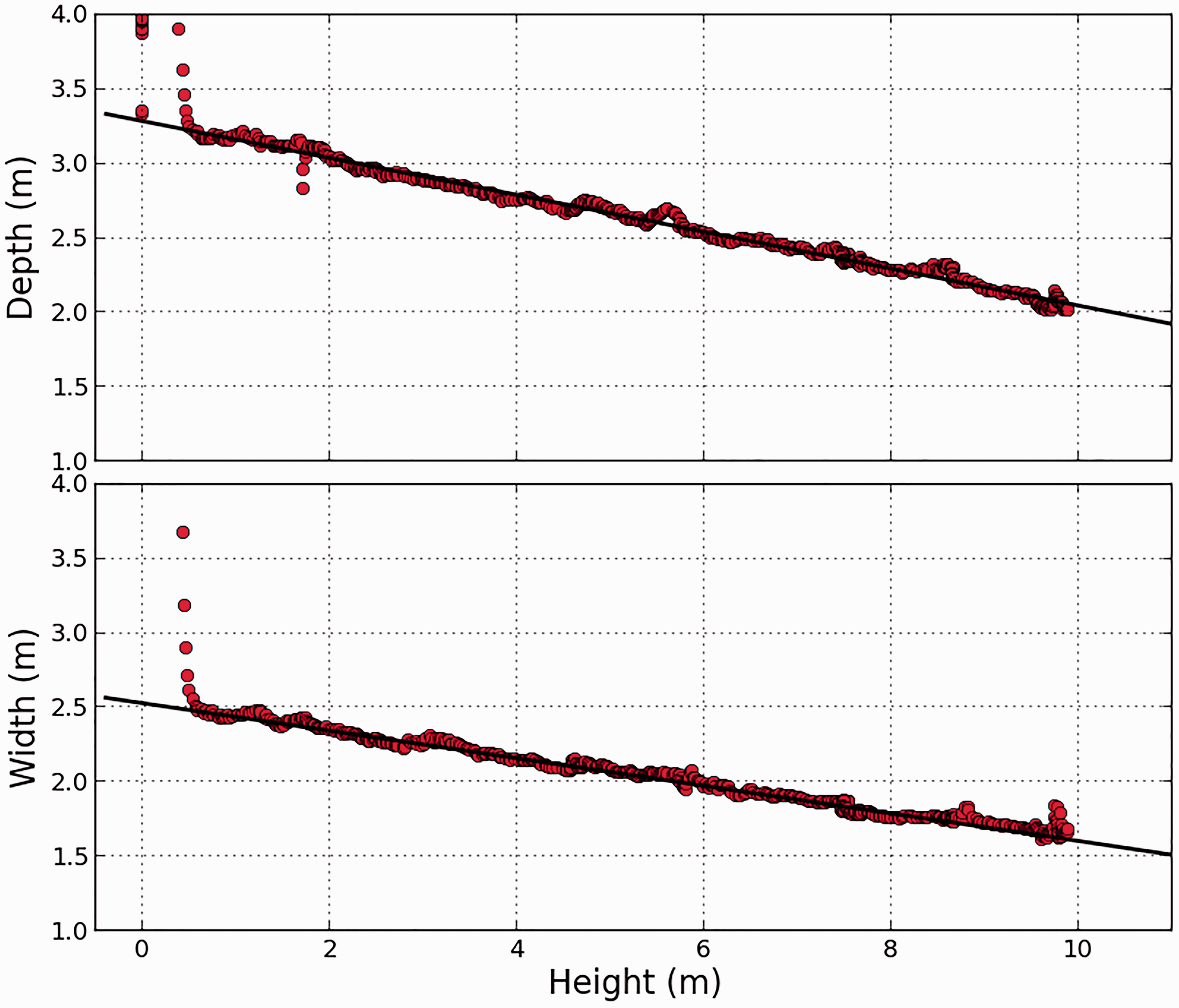
The estimated depth and width as a function of the height for the electric tower from Figure 3(a), fitted with straight lines.

Modelling the electric tower

A by-product of tracking the cross-section’s centre is the possibility of deriving a 3D representation of the electric tower from the observed data, such as a 3D point cloud reconstruction from the laser scans. A simple procedure consists in transforming each 2D scan into the estimated centre frame $\mathcal{C}$ , and projecting into 3D coordinates using the height measurements and the attitude estimates from the IMU measurements. This was tested on the same vertical flight data used to obtain Figure 11, and the final result is shown in Figure 12. Here, the efficiency of the tracking method is also evident, as the point cloud is capable of capturing a great amount of detail, and presents minimal deformations despite being made from data acquired on-flight.

Figure 12.

Partial 3D point cloud reconstruction of the electric tower from Figure 3(a), for a vertical flight in front of the tower. The laser scans are aligned using the tracked cross-section’s centre, the quadrotor’s altitude (from the laser altimeter) and attitude (from the IMU measurements).

A second possibility is to instead derive an abstract 3D geometric representation of the tower’s body from the estimated dimensions presented in Figure 11. A simple approach is to approximate each face as a planar segment, ⁶ and the edges of the tower as the intersection of adjacent planes m_j ( $j=1,\mathrm{\dots },4$ ), expressed as

$$m_j:a_{j}x+b_{j}y+c_{j}z+d_j=0,j=1,\dots ,4$$

(13)

where each m_j is associated with a face of the tower. Obtaining the planes’ coefficients results straightforward from Figure 11, as the slope of the fitted lines is directly related to the slopes of the planes. For example, for this particular case this resulted in

$$\{\begin{array}{cc}{m}_1:& -x-0.062z-1.643=0\\ m_2:& y-0.046z-1.265=0\\ m_3:& x-0.062z-1.643=0\\ m_4:& -y-0.046z-1.265=0\end{array}$$

(14)

which correspond to the front, right, back and left sides, respectively. With respect to an accurate point cloud reconstruction, which would require exploring extensive sections of the electric tower, this simplified planar representation can be obtained with more ease, as it only requires exploring a portion of the tower. As will be seen in the following sections, the main importance of these results is that both 3D representations of the tower can be exploited for pose estimation purposes.

Discussion

Since the final goal is to achieve autonomous navigation capabilities, all of the MAV’s 6 DoF must be determined. For this purpose, this proposed tracking approach could be complemented with additional sensing to recover complete 3D pose estimates, for example, using inertial measurements to estimate the roll and pitch angles, and an altitude sensor, such as a laser altimeter or a barometer. However, the constraints imposed on the MAV’s motion by this tracking approach are too restrictive for general inspection tasks that may require navigating continuously on all sides of the tower. An alternative strategy is thus to divide the inspection task into two steps. A first step consists in modelling the electric tower, which would allow to compensate for the limited information captured by the individual laser scans. The idea is to perform an initial vertical flight in front of the tower, in which our tracking algorithm is capable of providing a quantitative model of the tower (Figures 11 and 12). A second step would then focus on 3D pose estimation and navigation, using the estimated model to track the tower in general flight conditions. With such a model-based approach to recover pose estimates, the scan plane no longer needs to remain horizontal and less restrictions are imposed on the MAV’s movement. For the following sections, we consider that the first modelling step has already been performed based on our tracking approach, and instead focus the discussion on how to recover the complete 3D pose estimates.

3D local pose estimation

In this section, we present how to obtain complete 3D pose estimates with our sensor set-up. As is typically done with MAVs, the estimation process is broken down into several components.^15,17 Recalling that the complete 6 DoF pose from $\mathcal{B}$ to the inertial frame $\mathcal{I}$ is described by $\{x,y,z,\varphi ,\theta ,\psi \}$ , the 3D pose is reconstructed as follows: $\{x,y,\psi \}$ are estimated from the laser range measurements; then, as will be discussed, {z} is estimated from the laser range measurements fused with the barometer measurements; finally, $\{\varphi ,\theta$ } are obtained by fusing accelerometer and gyrometer measurements from the IMU. The following subsections explain each component of the estimation process.

We first explore how the classic ICP algorithm that has been successful indoors can be extended to the case of an electric tower inspection. This technique requires the surrounding environment to have sufficient geometric detail and is not suitable for highly unstructured scenarios often faced outdoors. ¹⁷ However, in an outdoor inspection scene, the rigid and well-defined structure of the electric towers has sufficient geometric detail to easily contrast from surrounding unstructured objects. This was exploited in the previous section to retrieve 2D pose estimates and will now be used to adapt the ICP algorithm. While common implementations focus on aligning pairs of scans to retrieve pose information in 2D, we instead treat the problem in 3D by introducing previous knowledge of the tower’s geometry in the registration process. We now present two possible implementations of the ICP algorithm.

Adapting the ICP algorithm: First proposed approach

In this first approach we follow a line of work typically adopted with the ICP algorithm in navigation tasks, consisting in aligning point clouds. The idea is to maintain the approach as general as possible, as no specific parameterization of the scene is required and pose information is recovered directly from the point correspondences. Let the current scan be represented by a set of 2D points, denoted $S_p=\{p_1,p_2,\dots ,p_{N_p}\}$ . For simplicity, consider that $S_p$ is expressed in the body-attached frame $\mathcal{B}$ . Then, let $S_q=\{q_1,q_2,\dots ,q_{N_q}\}$ denote the 3D reference set, expressed in the inertial frame $\mathcal{I}$ , which corresponds to a 3D point cloud reconstruction of the inspection scene, assumed to be acquired beforehand, e.g. from our tracking approach as discussed in the previous section. The goal is to find the rigid body transformation that best aligns $S_p$ to $S_q$ . The baseline ICP ²⁴ was used, with several modifications, notably in the minimization step. Each iteration k (starting from k = 0) is carried out as follows:

Initialization: The current estimate $T_{X_k}$ is used to transform all 2D points $p_i\in S_p$ into 3D coordinates in the inertial frame $\mathcal{I}$ , obtaining $S_{p\prime }$ . For the first iteration, the parameter vector is $X_0=(x_{\text{laser}},y_{\text{laser}},z_{\text{laser}},{\varphi }_{\text{imu}},{\theta }_{\text{imu}},{\psi }_{\text{laser}})$ , such that { $x_{\text{laser}},y_{\text{laser}},z_{\text{laser}},{\psi }_{\text{laser}}\}$ are obtained from the scan registration for the previous laser scan and $\{{\varphi }_{\text{imu}},{\theta }_{\text{imu}}\}$ from the IMU attitude estimation (as will be explained briefly).

Matching: Corresponding pairs $(p{\prime }_i,q_i)$ are established by associating each point in $S_{p\prime }$ to the closest point in $S_q$ . This correspondence search is the most time-consuming step of the algorithm. ²⁴ To speed up the matching process we make use of K–D trees, as is commonly done with ICP.^24,26

Rejection: Point pairs separated by more than a fixed distance threshold d_min are removed. This is mainly helpful with accuracy and stability in the presence of outliers, ²⁶ which in this case are typically due to surrounding vegetation.

Minimization: The goal is to find the transformation $T_{X_{\text{min}}}$ that minimizes the sum of squared errors, using the Euclidean distance as the distance metric. ²⁴ For the N remaining point pairs $(p{\prime }_i,q_i)$ , this leads to the following optimization problem

$$\begin{array}{c}{X}_{\text{min}}=\arg \underset{X}{\min }{\displaystyle \sum _{i=1}^N\left|\right|}{T}_x(p{\prime }_i)-q_i|{|}^2,\\ \text{such}\text{that\hspace{0.17em}}(\varphi ,\theta )=(0,0)\end{array}$$

(15)

which is solved with the Levenberg–Marquardt algorithm, since it allows to obtain accurate results and deal with initialization errors without significant speed losses. ⁴⁸ The components $\varphi$ and θ of $X$ are neglected during the minimization, since ${\varphi }_{\text{imu}}$ and ${\theta }_{\text{imu}}$ used at the initialization are precise and reliable. This reduces the optimization problem from a 6D space to a 4D space, which further limits the risk of divergence due to local minima, and provides a more reliable solution. This is the main modification of the algorithm.

• 5. Finally, the current estimate is updated as

  $$T_{X_{k+1}}=T_{X_{\text{min}}}·T_{X_k}$$

  (16)

Due to the previous step, $T_{X_{\text{min}}}$ only updates the { $x,y,z,\psi \}$ components of $T_{X_k}$ in each iteration.

The end result of the scan registration process is an estimation of the 3D translation vector $(x_{\text{laser}},y_{\text{laser}},z_{\text{laser}})$ and the yaw angle ${\psi }_{\text{laser}}$ . The main novelty is thus that altitude estimates can now be recovered, which is a direct consequence of introducing a 3D point cloud reconstruction of the tower in the registration process.

Limitations

Besides the drawbacks inherent to the ICP algorithm discussed at the beginning of this article, other limitations can be pointed out. Evidently, this approach is restricted to sections of the tower captured in the 3D point cloud reconstruction. Pose estimates cannot be recovered in previously unexplored or occluded sections. For this approach to be effective, the 3D point cloud must accurately capture the complete electric tower, which is a complex task. With our tracking algorithm from the previous section this requires exploring extensive portions of the tower. Other existing solutions rely on offline processing of data from powerful and expensive 3D LiDARs capable of capturing dense measurements from long distances.^6,19 This, however, goes beyond the scope of this work.

Further complications arise regarding the altitude estimates. For a 2D LiDAR, measurements from the individual scans fall within the same plane and do not directly capture the MAV’s altitude, which is instead determined from the point correspondences with the 3D point cloud uniquely. The altitude estimates are thus more unreliable and prone to errors, as will be seen in the simulation results. Furthermore, altitude estimation is highly dependent on the inclination of the faces of the tower. In the worst-case scenario, no altitude information can be recovered for completely vertical faces, which is a situation rarely faced with high voltage electric towers considered in this work. These drawbacks justify the use of an additional barometer sensor. However, as will be seen, this proposed ICP implementation will overall perform well if the electric tower remains within the sensor’s field of view, and particularly stable results can be achieved for near-hovering conditions. This quality holds for altitude estimates and will be exploited to track the barometer drift.

Adapting the ICP algorithm: Second proposed approach

The difficulties in obtaining an accurate 3D point cloud reconstruction of the inspection scene can render the previous approach impractical. Nonetheless, the ICP algorithm can be applied to a wide variety of representations of geometric data such as line sets, triangle sets, parametric surfaces, among others. ²⁴ Therefore, an alternative is to align the laser scans onto the simplified planar representation of the tower body from equation (13), which is simpler to obtain than a complete point cloud reconstruction, as previously discussed. To achieve this, we adopt a projection-based matching strategy,^49,50 where, after initialization, the corresponding points $q_i$ are calculated as the orthogonal projection of every point $p{\prime }_i\in S_{p\prime }$ onto the closest planar segment from m_j. This substitutes the time-consuming correspondence search previously used, and, as will be seen, allows obtaining significant speed gains. ²⁶

Thus, in this approach, the matching step (step 2) for each point $p{\prime }_i$ is now carried out as follows:

For the tower face m_j (starting with j = 1), calculate the two edge lines ${\mathcal{L}}_A$ and ${\mathcal{L}}_B$ as the intersection with the two adjacent planes.

Project $p{\prime }_i$ orthogonally to the plane equation of m_j (equation (13)), obtaining $q$ . We have to determine if $q$ falls within the planar segment delimited by ${\mathcal{L}}_A$ and ${\mathcal{L}}_B$ . This is done as follows:

•  – Project $p_i\prime$ to the edge lines ${\mathcal{L}}_A$ and ${\mathcal{L}}_B$ , obtaining $q_A$ and $q_B$ , respectively.

•  – Let $\overline{AB}=q_B-q_A$ .

•  – Calculate the normalized projection $\rho =\frac{(q-q_A)·(\overline{AB})}{\left|\right|\overline{AB}|{|}^2}$ .

•  – If $0<\rho <1$ , then $q$ falls within the planar segment, and the projection is $q$ .

•  – If $\rho \le 0$ , then $q$ falls outside of the planar segment and the projection is $q_A$ .

•  – If $\rho \ge 1$ , then $q$ falls outside of the planar segment and the projection is $q_B$ .

These steps are repeated for the four faces of the tower, and the projected point which yields the minimum distance to $p_i\prime$ is chosen as the corresponding point $q_i$ . Then, the remaining steps from the previous implementation are left unchanged. As before, the output is $(x_{\text{laser}},y_{\text{laser}},z_{\text{laser}},{\psi }_{\text{laser}})$ .

Limitations

One of the main drawbacks of this formulation is that it applies specifically to the case of rectangular cross-sections. The projection strategy would have to be changed for a different tower geometry. In contrast, the point cloud approach is more general in this matter and would not require any modifications. As before, no altitude information can be recovered if the faces of the tower are completely vertical.

Altitude estimation

The altitude estimates obtained previously from the laser range measurements have a strong dependence on the shape of the tower and can result unreliable. In contrast, barometer measurements are independent from the shape of surrounding structures, but suffer from drift over time due to varying atmospheric conditions. Here, we seek to combine both sources of altitude information in order to tackle their respective drawbacks. We first recall the MAV's vertical dynamics with respect to an inertial frame $\mathcal{I}$ from equation (4)

$$\{\begin{array}{c}\dot{z}=v_z\\ {\dot{v}}_z=g+\frac{F_z}{m}\end{array}$$

(17)

Accurate vertical velocity estimates can be obtained by fusing the barometer and IMU measurements,^31,32 and are thus obtained separately, as will be addressed in a later discussion. Therefore, in this section we consider that v_z is a known input, and instead use the following system

$$\{\begin{array}{c}\dot{z}=v_z\\ {\dot{b}}_z=0\end{array}$$

(18)

where b_z is the unknown barometer drift, which is modelled as a constant as it varies slowly in time, and is defined by the relationship $z_{\text{baro}}=z+b_z$ , with $z_{\text{baro}}$ denoting the barometer measurement. This leads to a simple second-order feedback observer formulation

$$\{\begin{array}{c}\dot{\widehat{z}}=v_z-k_z(\widehat{z}-{\overline{z}}_1)\\ {\dot{\widehat{b}}}_z=-k_{b_z}(\widehat{z}-{\overline{z}}_2)\end{array}$$

(19)

where $(k_z,k_{b_z})$ are the estimation gains, and ${\overline{z}}_n$ is an auxiliary variable defined as

$$\begin{array}{c}{\overline{z}}_n={\lambda }_n(z_{\text{baro}}-{\widehat{b}}_z)+(1-{\lambda }_n)z_{\text{laser}}\text{with}0\le {\lambda }_n\le 1,\\ n=1,2\end{array}$$

(20)

which is the weighted sum of the laser altitude estimates $z_{\text{laser}}$ and barometer readings $z_{\text{baro}}$ compensated for bias. The weights λ_n allow one to determine how each sensor contributes to the estimation of each state. In particular, as λ_n increases, higher priority is given to the barometer readings. The reasoning behind this parameterization is to use the laser estimates mainly to keep track of slowly varying barometer bias ${\widehat{b}}_z$ and to maintain the more reliable barometer measurements to estimate $\widehat{z}$ . Choosing the weights ${\lambda }_1=1$ and ${\lambda }_2=0$ achieves this purpose. The stability analysis for this observer and details on how to tune the gains $(k_z,k_{b_z})$ are given in Appendix 1.

Attitude estimation

We now present our proposed non-linear observer formulation using the accelerometer and gyroscope measurements. As yaw estimates are already obtained from the laser scan registration, the main goal is to recover estimates of the roll $\varphi$ and pitch θ angles. First, let $\text{γ}={({\gamma }_1,{\gamma }_2,{\gamma }_3)}^{\mathrm{⊺}}$ denote the vertical axis of $\mathcal{I}$ expressed in $\mathcal{B}$ as

$$\text{γ}=R^{\mathrm{⊺}}{e}_3$$

(21)

with $e_3={(0,0,1)}^{\mathrm{⊺}}$ . From the rotation matrix definition of equation (1), it follows that $\text{γ}$ contains implicitly the MAV’s roll and pitch angles, since

$$\begin{array}{c}\varphi =\arcsin \left({\gamma }_2\right)\\ \theta =\text{atan2}\left(-{\gamma }_1,{\gamma }_3\right)\end{array}$$

(22)

Recalling that a MAV’s rotational kinematics is given by ³³

$$\dot{R}=RS(\text{ω})$$

(23)

with $S(.)$ the skew-symmetric matrix associated with the cross-product (i.e. $S(x)y=x\times y,\forall x,y\in {\mathbb{R}}^3$ ), and $\text{ω}$ the angular velocity vector from $\mathcal{B}$ to $\mathcal{I}$ , expressed in $\mathcal{B}$ . Then, the kinematics of $\text{γ}$ can be deduced from equations (21) and (23), and results in

$$\dot{\text{γ}}=\text{γ}\times \text{ω}$$

(24)

This is the basis of our observer formulation. As previously mentioned, the goal is to recover roll and pitch estimates from the gyrometer and accelerometer readings. Let $a_m$ denote the accelerometer measurements expressed in $\mathcal{B}$ , which measure the specific acceleration acting on the MAV’s airframe ³³

$$a_m=R^{\mathrm{⊺}}(\dot{\text{v}}-g{\text{e}}_3)=R^{\mathrm{⊺}}\dot{\text{v}}-g\text{γ}$$

(25)

Then, under the assumption of negligible linear acceleration, one has ³⁵

$$a_m\approx -g\text{γ}$$

(26)

which shows that accelerometers provide direct observations of the roll and pitch angles (and of $\text{γ}$ ). Thus, the following non-linear observer for $\text{γ}$ is proposed

$$\stackrel{.}{\widehat{\text{γ}}}=\widehat{\text{γ}}\times ({\text{ω}}_m-k_{\gamma }(a_m\times \widehat{\text{γ}})),k_{\gamma }>0$$

(27)

with ${\text{ω}}_m$ the angular velocities measured by the gyrometer in $\mathcal{B}$ .

To analyse the stability of this estimator, consider the candidate Lyapunov function $L=1-{\text{γ}}^T\widehat{\text{γ}}$ . From equations (26) and (27) one has

$$\stackrel{.}{\widehat{\text{γ}}}\approx \widehat{\text{γ}}\times \left({\text{ω}}_m-k_{\gamma }g(\widehat{\text{γ}}\times \text{γ})\right)$$

(28)

Then, assuming that this approximation of $\stackrel{.}{\widehat{\text{γ}}}$ is perfect, and that ${\text{ω}}_m=\text{ω}$ , it can be proven that $\dot{L}=-k_{\gamma }g\left|\right|\widehat{\text{γ}}\times \text{γ}|{|}^2$ , which is decreasing along the solutions of the system if, initially, $\widehat{\text{γ}}$ and $\text{γ}$ are not opposite to each other, and $k_{\gamma }>0$ . This implies in particular the convergence of $\widehat{\text{γ}}$ to $\text{γ}$ .

Gain scheduling

The approximation from equation (26) is commonly used in attitude estimation when dealing with accelerometers, ³⁵ but only holds when flying at constant velocity or near stationary flight conditions. An added benefit of non-linear observer formulations is that the estimation gains can be tuned in real time during flight. ³³ This can be exploited to adapt the observer to changing dynamic conditions, in particular, to high acceleration states where the assumption from equation (26) is no longer valid and estimation performance is deteriorated. In such situations, which typically last for short periods of time, it is better to lower the estimation gains and to rely on the gyrometer measurements since they are scarcely affected by the linear accelerations, ⁵¹ and can provide short-term rotations accurately. ³⁸

A basic strategy is thus to detect highly accelerated states by comparing the magnitude of the accelerometer readings to the gravity acceleration.^36,37,51 Let ${\tilde{a}}_m$ denote the absolute accelerometer measurement error with respect to gravity as

$${\tilde{a}}_m=\left|\right|\left|{\text{a}}_m\right||-g|,g=9.81\frac{m}{s^2}$$

(29)

This magnitude provides a simple criteria to determine the dynamic state of the MAV, as ${\tilde{a}}_m\approx 0$ for near-hovering conditions, and large values of ${\tilde{a}}_m$ correspond to highly dynamic motion. The estimation gains can then be adapted accordingly. Yoo et al. ³⁶ adopt a simple switching strategy to choose the gain between a set of nominal values corresponding to no-acceleration, low-acceleration or high-acceleration states. Instead, Valenti et al. ⁵¹ set a nominal gain for hovering state, which is then decreased linearly during transitions to high acceleration states. We adopt a strategy similar to Valenti et al. ⁵¹ Let k_L and k_H denote the nominal gains during low- and high-acceleration states, respectively; the idea is to transition smoothly between these gains. The following gain scheduling approach is proposed

$$k_{\gamma }({\tilde{a}}_m)=k_L{e}^{-\alpha {\tilde{a}}_m}+k_H(1-e^{-\alpha {\tilde{a}}_m}),\alpha >0$$

(30)

where α is an arbitrary positive constant that determines the steepness of the transitions between k_L and k_H. It is simple to verify that as ${\tilde{a}}_m\approx 0$ , then $k_{\gamma }$ remains near k_L, and as ${\tilde{a}}_m$ increases, then $k_{\gamma }$ decreases towards k_H, which is the desired behaviour. This is further illustrated in Figure 13 for $k_L=0.1,k_H=0.01$ and different values of α. It can be noted that α = 0 corresponds to the constant gain case, and as α increases, the gains decrease faster towards k_H.

Figure 13.

An example of the attitude observer gains according to equation (30), for different values of α.

Complete rotation matrix reconstruction

The estimated roll ${\varphi }_{\text{imu}}$ and pitch ${\theta }_{\text{imu}}$ angles are recovered from $\widehat{\text{γ}}$ and equation (22) as

$$\begin{array}{c}{\varphi }_{\text{imu}}=\arcsin \left({\widehat{\gamma }}_2\right)\\ {\theta }_{\text{imu}}=\text{atan2}\left(-{\widehat{\gamma }}_1,{\widehat{\gamma }}_3\right)\end{array}$$

(31)

Finally, the complete estimated rotation matrix $\widehat{R}$ is recovered by combining the estimated angles as

$$\widehat{R}=R_z({\psi }_{\text{laser}})R_x({\varphi }_{\text{imu}})R_y({\theta }_{\text{imu}})$$

(32)

This matrix is subsequently used at each initialization of the laser scan registration, and for the velocity estimation described in the following section.

Velocity estimation

In the previous section, the complete six DoF pose of the MAV was determined from the sensor measurements. The goal is now to derive velocity estimates by combining the pose estimates with the inertial measurements from the IMU. For this purpose, we make use of the translational dynamics of the MAV with respect to the inertial frame $\mathcal{I}$ from equation (3) to formulate velocity observers. In the following analysis, the external aerodynamic forces $F={(F_x,F_y,F_z)}^{\mathrm{⊺}}$ from equation (4) are determined from the accelerometer readings ${\text{a}}_m$ and the estimated attitude $\widehat{R}$ as

$$F=m\widehat{R}{\text{a}}_m$$

(33)

Since different sensors are used for the different states, the horizontal and vertical velocity components are analysed separately.

Horizontal velocity estimation

From equation (4) it follows that the dynamics for {x, y} in $\mathcal{I}$ are two independent second-order systems. Estimating the horizontal velocities results straightforward and is achieved with simple feedback state observers defined as

$$\begin{array}{c}\{\begin{array}{cc}\dot{\widehat{x}}={\widehat{v}}_x-k_x(\widehat{x}-x_{\text{laser}})& \\ {\dot{\widehat{v}}}_x=\frac{F_x}{m}-k_{v_x}(\widehat{x}-x_{\text{laser}}),& k_x,k_{v_x}>0\end{array}\\ \{\begin{array}{cc}\dot{\widehat{y}}={\widehat{v}}_y-k_y(\widehat{y}-y_{\text{laser}})& \\ {\dot{\widehat{v}}}_y=\frac{F_y}{m}-k_{v_y}(\widehat{y}-y_{\text{laser}}),& k_y,k_{v_y}>0\end{array}\end{array}$$

(34)

where $(k_x,k_{v_x})$ and $(k_y,k_{v_y})$ are the scalar observer gains, which guarantee exponential convergence if they are positive, and $(x_{\text{laser}},y_{\text{laser}})$ are the estimates obtained from the laser scan registration described in the previous section.

Vertical velocity estimation

As previously mentioned, satisfying estimates of the vertical velocity can be recovered from barometer and accelerometer measurements.^31,32 As will be seen, these estimates remain accurate even in the presence of barometer drift. Recalling the vertical dynamics from equation (17), we now formulate the following feedback state observer

$$\{\begin{array}{cc}\dot{\widehat{z}}={\widehat{v}}_z-k_z(\widehat{z}-z_{\text{baro}})& \\ {\dot{\widehat{v}}}_z=g+\frac{F_z}{m}-k_{v_z}(\widehat{z}-z_{\text{baro}}),& k_z,k_{v_z}>0\end{array}$$

(35)

where $(k_z,k_{v_z})$ are the observer gains, and $z_{\text{baro}}$ are the barometer altitude measurements. The altitude estimates from the laser scan registration are not included as they only degrade the performance. The vertical velocity estimates ${\widehat{v}}_z$ are subsequently used as an input to the altitude observer from equation (19).

Simulation results: 3D local pose estimation

The purpose of this section is to assess the performance of the different components of the pose estimation process. The results presented here were obtained from simulated flights carried out using the previously discussed simulation set-up, illustrated in Figure 3(b). For the flights, a set of waypoints was given for the quadrotor to follow, accounting for a complete displacement around the tower. Meanwhile, the MAV’s yaw angle was oriented towards the centre of the tower, so that the latter remains in the LiDAR’s field of view. Since the focus of this section is to assess the quality of the pose estimates, the simulation ground truth is directly used to stabilize the MAV’s position and attitude. The complete flight is shown in Figure 14.

Figure 14.

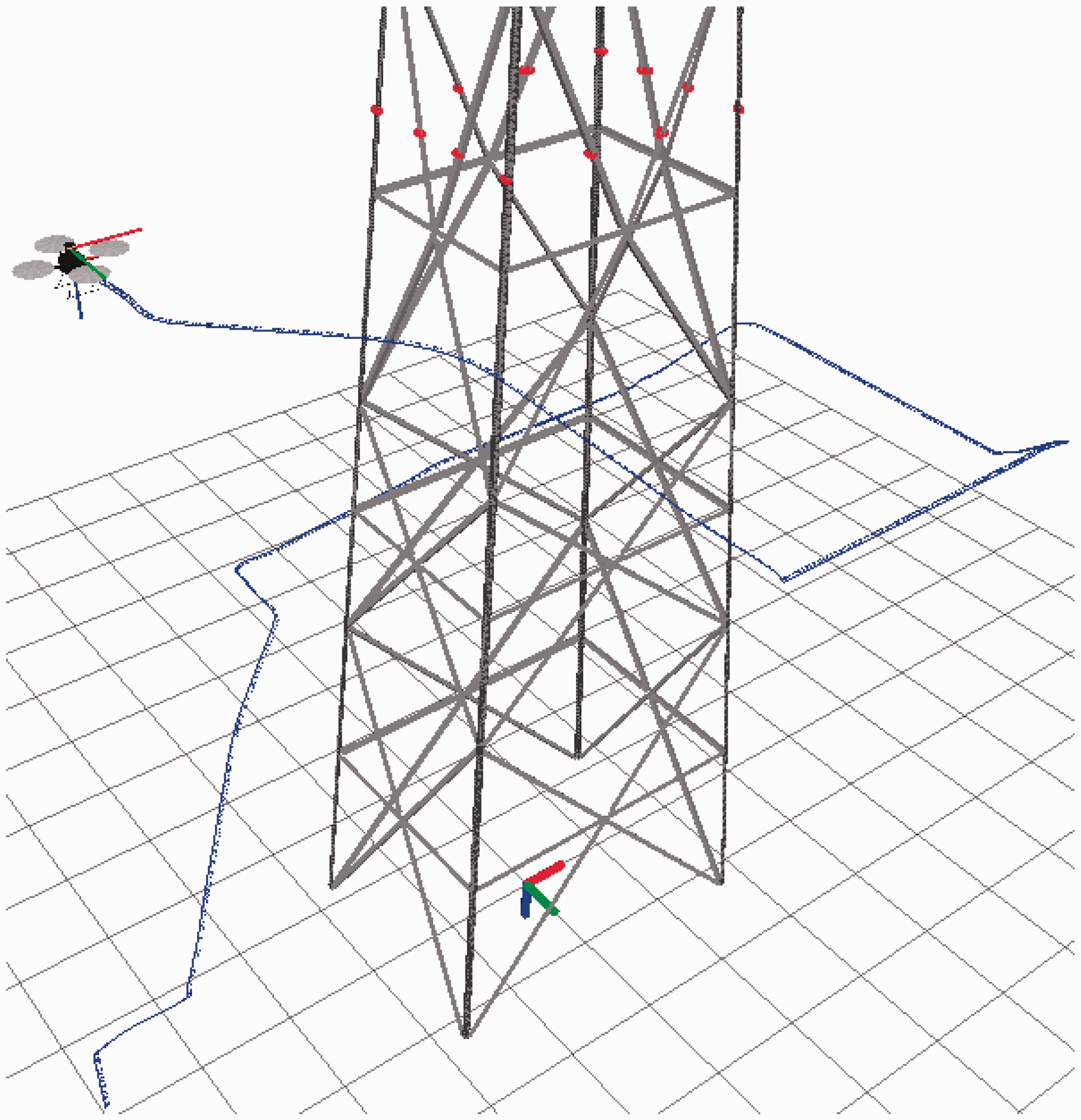
The simulated flight around the tower. The blue line indicates the trajectory. Throughout the flight the quadrotor was oriented towards the centre of the tower.

Attitude estimation results

The attitude observer from equation (27) was used to fuse the accelerometer and gyrometer measurements and recover estimates of the roll and pitch angles $\{\varphi ,\theta \}$ . We now analyse the performance of this observer throughout the flight. Figure 15(a) illustrates the deviations of the accelerometer readings from the acceleration of gravity ( ${\tilde{a}}_m$ from equation (29)) for a portion of the flight. As can be seen, the MAV spends larger amounts of time in low acceleration states ( ${\tilde{a}}_m\approx 0$ ). Then, the peaks correspond to instants when the MAV accelerates towards a different waypoint. The idea is to adapt the observer to these peaks by lowering the estimation gain $k_{\gamma }$ . This was carried out with the gain scheduling approach from equation (30). Based on results observed in the simulations, the nominal gains were set to $k_L=0.1$ and $k_H=0.01$ . Moreover, the estimation process was repeated for different values of the parameter α, from α = 0, which corresponds to the constant gain case since $k_{\gamma }=k_L$ (from equation (30)), to α = 100. As explained, this parameter determines the steepness of the transitions between the two nominal gains. The resulting scheduled gains for a portion of the flight are shown in Figure 15(b). When comparing the two figures, it can be noted the gain $k_{\gamma }$ rapidly drops in the presence of acceleration peaks (e.g. $t=26\text{s}$ and $t=30\text{s}$ ), which is the desired behaviour. However, as α increases, the gains can result overly sensitive to small changes in ${\tilde{a}}_m$ ( $t=38\text{s}$ for α = 100).

Figure 15.

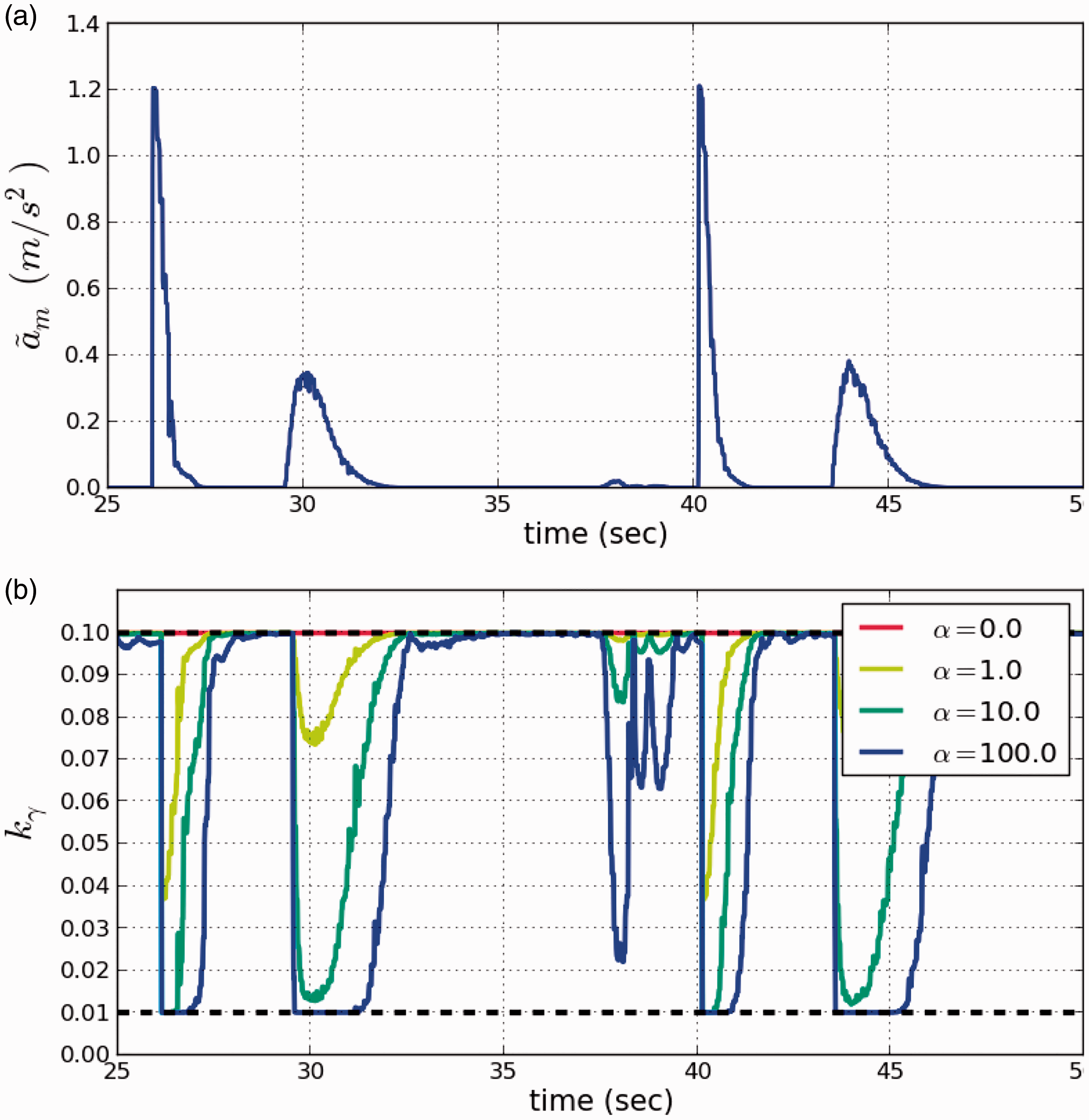
For a portion of the flight from Figure 14: (a) The deviations of the accelerometer readings from gravity according to equation (29). (b) The resulting scheduled gains for different values of α. The gains become more reactive for larger values of α.

Next, the absolute estimation errors with respect to the simulation ground truth are shown in Figure 16(a) and (b) for the roll and pitch angles, respectively. On the one hand, when comparing Figure 16(a) and (b) to (c), it can be noted that the observer can accurately trace the roll and pitch angles in low acceleration states (when ${\tilde{a}}_m\approx 0$ ) for all cases, and the errors for the most part remain below $1^{°}$ . On the other hand, the largest estimation errors correspond to peaks in ${\tilde{a}}_m$ (e.g. $t=26\text{s}$ and $t=40\text{s}$ ), reaching a maximum for the constant gain observer of ${2.45}^{°}$ for the roll angle, and ${2.62}^{°}$ for the pitch angle. In contrast, as the parameter α is increased, error peaks related to ${\tilde{a}}_m$ are now largely suppressed and the overall performance is improved with the simple gain scheduling strategy. Based on these results, a gain scheduled attitude estimation with α = 10 was used for the following sections, as it offers a good trade-off between sensibility to changes in ${\tilde{a}}_m$ and estimation error reduction.

Figure 16.

For the attitude observer from equation (27) and different values of α: (a) Absolute roll estimation error, (b) absolute pitch estimation error and (c) the corresponding ${\tilde{a}}_m$ . As α increases, the errors caused by peaks in ${\tilde{a}}_m$ are reduced.

Laser-based local pose estimation results

The two proposed implementations of the ICP algorithm were tested in the simulations to recover estimates of the remaining states $\{x,y,z,\psi \}$ . In the first case, the laser scans were aligned to the 3D point cloud reconstruction shown in Figure 17(a), which was obtained beforehand from the simulated tower shown in Figure 3(b), following the same procedure for Figure 12 based on our tracking approach. In the second case, the laser scans were instead aligned to the planar representation of the tower illustrated in Figure 17(b), which was also obtained beforehand following the procedure used for Figure 11 and equation (14), relying on our tracking approach. Here, the estimated coefficients from equation (7) resulted in

$$\{\begin{array}{cc}{m}_1:& -x-0.076z-1.749=0\\ m_2:& y-0.046z-1.219=0\\ m_3:& x-0.076z-1.749=0\\ m_4:& -y-0.046z-1.219=0\end{array}$$

(36)

which correspond to the front, right, back and left sides, respectively. In both ICP implementations, an initial rough knowledge of the MAV’s position with respect to the tower was given for the first scan registration. For each subsequent laser scan, the estimation process was initialized with the results from the previous scan registration and attitude estimates from the IMU measurements.

Figure 17.

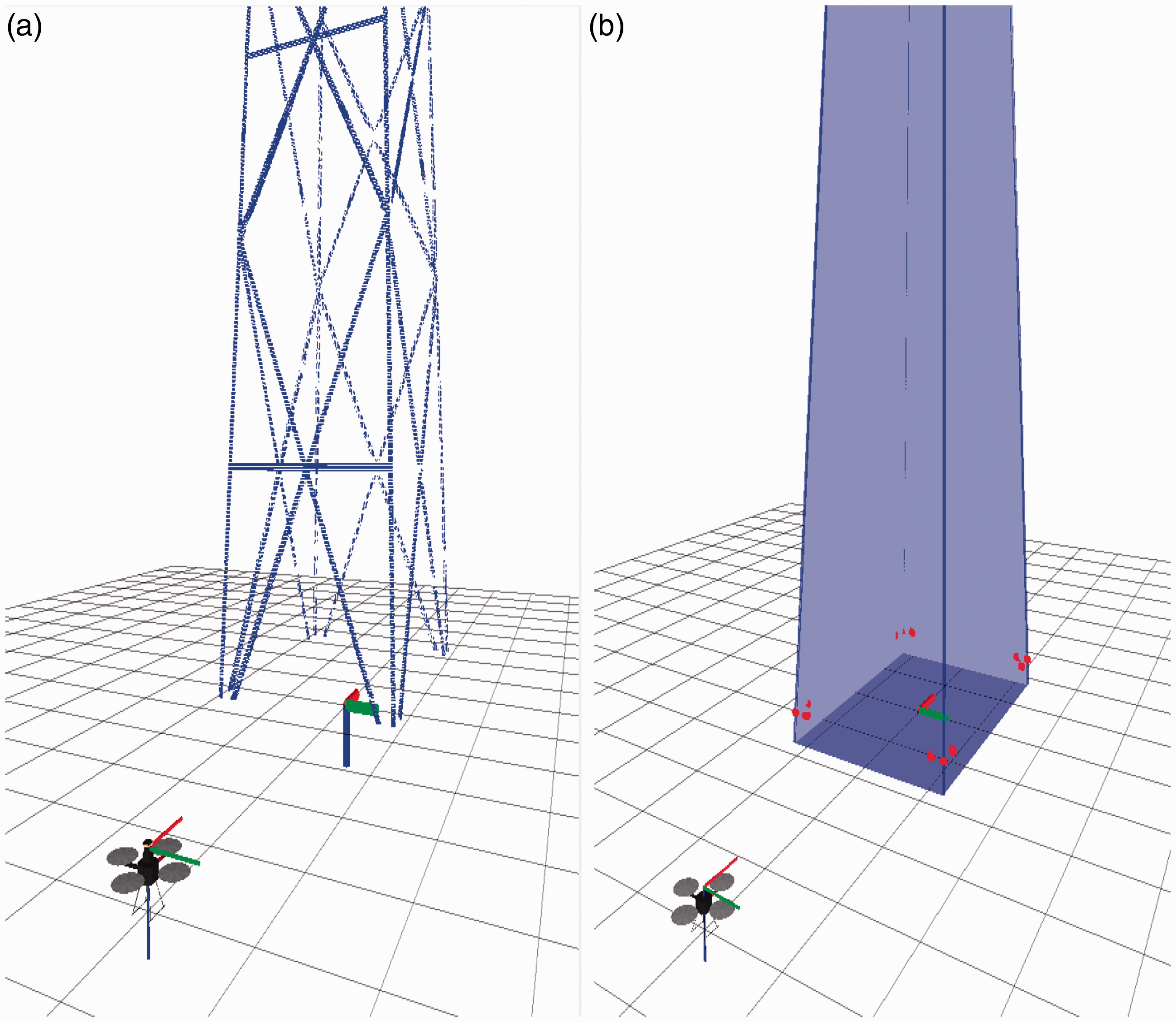
The two models used as reference in the ICP algorithm to align the laser scans: (a) Point cloud reconstruction and (b) planar model.

We now analyse the performance of the two approaches. First, the computation time required for the scan registration in both cases is shown in Figure 18. As expected, using the planar model results in significantly faster estimates with an average of $1.4\text{ms}$ , compared to the point cloud case average of $16\text{ms}$ . This shows the effectiveness of the projection-based matching strategy used to establish point correspondences, which avoids the computationally extensive correspondence search required for the point cloud registration.

Figure 18.

Comparing the computation time for the laser scan registrations. The planar model approach is approximately 10 times faster. ICP: iterative closest point.

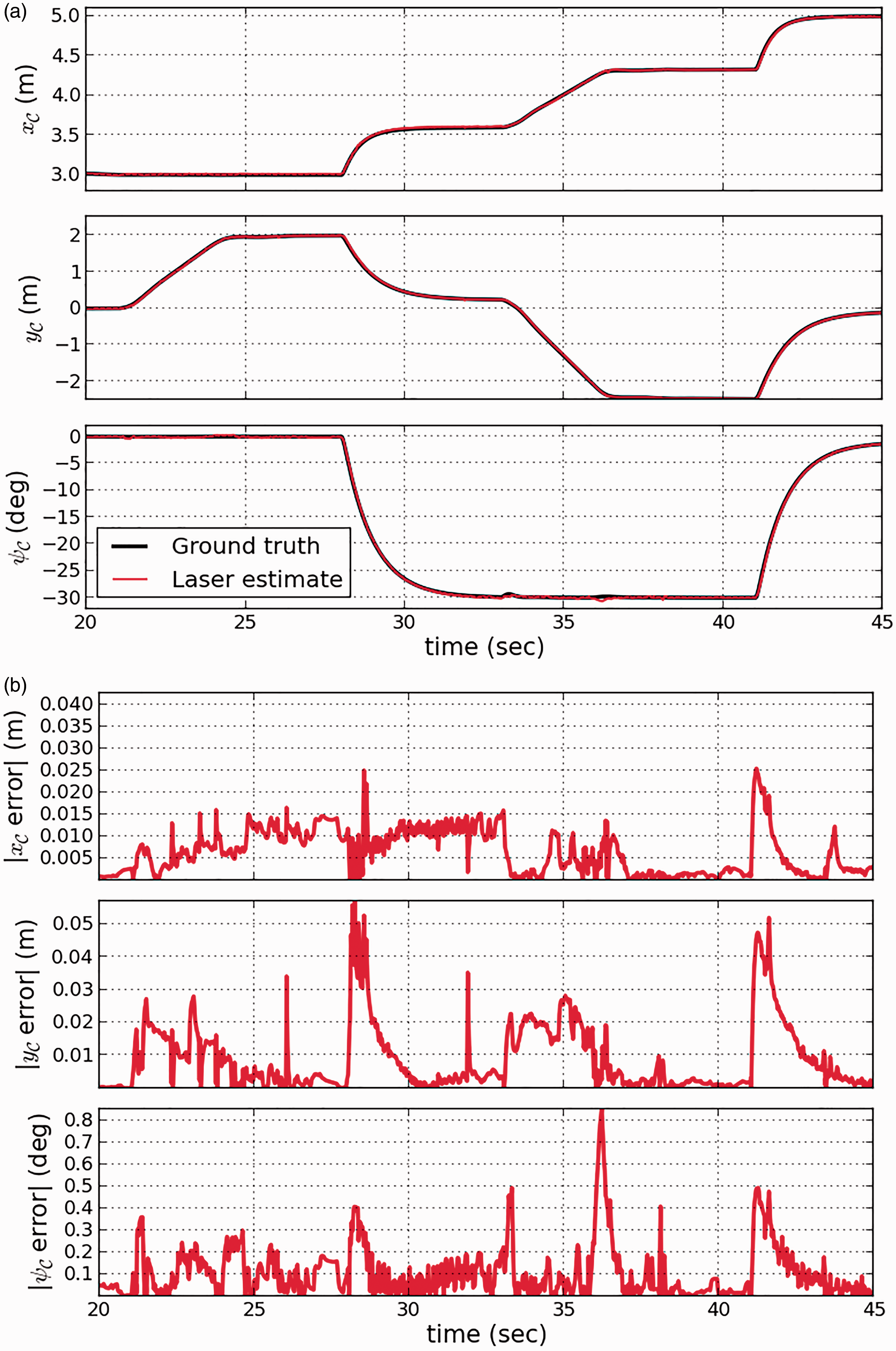
Next, Figure 19 compares the MAV’s ground truth position with the estimates from both approaches. As can be seen, the results obtained with the planar model approach effectively follow the ground truth for the duration of the flight. However, the point cloud approach ultimately fails before completing the flight. This can be further observed from the absolute errors shown in Figure 20. For the planar model case, the {x, y} errors remain below $5\text{cm}$ (Figure 20(a) and (b)). Furthermore, the yaw estimates are also very precise, with a maximum error of ${0.8}^{°}$ (Figure 20(d)). In these figures it can be noted that the point cloud approach achieves similar performance before failing (near $t=40\text{s}$ ). Then, particular attention must be given to the altitude estimation errors from Figure 20(c). As previously pointed out, the horizontally placed 2D laser scanner captures very limited altitude information. As a result, it was observed throughout the simulations that the altitude estimates were easily deteriorated in complicated situations, for example, when the horizontal bars on the tower block most of the sides from the sensor’s view (as in Figure 4(d)). For the planar model case, this typically caused spurious estimates, with the absolute error jumping above $20\text{cm}$ (e.g. $t=20\text{s}$ and $t=30\text{s}$ in Figure 20(c)). For the point cloud case, this eventually caused the approach to completely fail (around $t=30\text{s}$ in Figure 20(c)). Despite these complications, in Figure 20(c) it can be observed that the altitude errors remain at acceptable levels below $10\text{cm}$ throughout most of the flight for the planar case, and similarly for the point cloud approach before failure. Properly exploiting the limited altitude information requires special attention and is addressed in the following section.

Figure 19.

Comparing the ICP position estimates with the ground truth, for the simulated flight from Figure 14. The point cloud approach fails before finishing the flight. ICP: iterative closest point.

Figure 20.

Absolute estimation errors with respect to the simulation ground truth for the results from Figure 19, for both implementations of the ICP algorithm. ICP: iterative closest point.

Altitude estimation results

We now present the results for the altitude observer from equation (19), which fuses the laser altitude estimates from both implementations of the ICP algorithm with the barometer measurements. Barometer readings are sensitive to changes in atmospheric conditions (strong winds, temperature changes), which generally translates into a slowly varying drift. In order to study the observer’s behaviour under large barometer drift, this was simulated as a sinusoid with a maximum speed of 1 m/min. As previously mentioned, the weights from equation (20) were chosen as ${\lambda }_1=1$ , to rely mainly on the barometer measurements to estimate the altitude, and ${\lambda }_2=0$ , to rely on the laser estimates to estimate the barometer drift. Then, the estimation gains were set to $(k_z,k_{b_z})=(6.6,-1.36)$ , which achieved a good performance in the simulations. An explanation on how to determine these gains is given in Appendix 1. In these simulations, the observer’s output was used at each scan registration initialization, instead of the laser altitude estimates. The impact of this can be observed in Figure 21, where the complete position estimates of the ICP implementations are once again compared to the simulation ground truth. In contrast to the results from Figure 19, it can be noted that the introduction of the altitude observer allows correcting the large altitude errors that previously caused the point cloud case to fail, which now offers a similar performance to the planar model case. Furthermore, Figure 22 presents a comparison of the absolute errors of the barometer measurements, the altitude estimates of the ICP algorithm (without the aid of the observer) and the altitude observer’s output. In both cases it can be noted that, while the barometer readings accumulate a large error over time, the presence of this drift does not significantly degrade the quality observer’s altitude estimates, which instead provides notable improvements. For the planar model case in Figure 22(a), the spurious error peaks are largely filtered, and the maximum error is lowered to $10\text{cm}$ . More importantly, for the point cloud case in Figure 22(b), the observer manages to avoid failing at $t=30\text{s}$ and provides continuous estimates throughout the entire flight. The effectiveness of this formulation is further verified in Figure 23, as the observer manages to estimate the previously unknown barometer drift, with less than $10\text{cm}$ of error.

Figure 21.

The ICP position estimates after introducing the altitude observer. The large altitude errors are corrected and the point cloud approach no longer fails. ICP: iterative closest point.

Figure 22.

The absolute altitude errors for ICP without the aid of the altitude observer, the barometer measurements with drift and the altitude observer for (a) ICP with planar model and (b) ICP with point cloud reconstruction. ICP: iterative closest point.

Figure 23.

For the altitude observer and both ICP implementations: (Top) Comparing the barometer drift estimates with the ground truth. (Bottom) Absolute estimation errors. The observer succeeds in both cases.

Simulation results: Velocity estimation

Horizontal velocity estimation results

The {x, y} estimates from the laser scan registration were used as an input to the velocity observers from equation (34), where they were fused with the accelerometer readings to recover the horizontal velocity estimates. The estimation gains were chosen identical for both axis as $(k_x,k_{v_x})=(6.4,16)$ and $(k_y,k_{v_y})=(6.4,16)$ . The estimated horizontal velocities for a portion of the flight and both implementations of the ICP algorithm are shown in Figure 24. For both axes, the high estimation gains allow the speed estimates to converge fast towards the ground truth. Furthermore, the good quality of the position estimates from the scan registration allows the velocity errors to remain below $10\frac{\text{cm}}{\text{s}}$ .

Figure 24.

Horizontal velocity estimation results for the observer from equation (34). (a) x-component (Vx) and (b) y-component (Vy).

Vertical velocity estimation results

Finally, the observer from equation (35) was used to recover vertical velocity estimates from the barometer and accelerometer readings. As before, the observer gains were chosen as $(k_z,k_{v_z})=(6.4,16)$ . Figure 25(a) shows the estimation results without barometer drift. As can be seen, the vertical velocity estimates are sufficiently accurate without the need of the laser estimates, as they remain below $1.5\frac{\text{cm}}{\text{s}}$ . Then, the velocity estimates in the presence of barometer drift are shown in Figure 25(b). With respect to the previous case, the estimation error slightly increases but remains within acceptable levels.

Figure 25.

Vertical velocity estimates (Vz) obtained by fusing barometer and IMU measurements. (a) Without barometer drift and (b) with barometer drift.

Conclusions and future work

In this article we have presented a methodology to recover complete 3D pose estimates in electric tower inspection tasks with MAVs, using a sensor set-up consisting of a 2D LiDAR, a barometer sensor and an IMU. First, we addressed 2D local pose estimation using uniquely the laser range measurements. Basic geometric knowledge of the tower was used to extract the notable features captured in the individual laser scans, which were then used to track the cross-sections and to estimate their previously unknown dimensions. Simulations yielded satisfying results under simple flight conditions, but the assumptions used by this approach proved too restrictive for general inspection tasks. It was shown that this tracking method could instead be used with additional sensing to model the tower. This was tested on data acquired from real flights, and results were presented for a partial point cloud reconstruction of the tower’s body and a simplified planar representation derived from the dimensions estimated on-flight. The inspection task was thus divided into two steps, tower modelling and pose estimation.

Then, we focused on 3D local pose estimation using the complete sensor set-up, which was divided into three components. At the lowest level, a non-linear observer formulation to estimate the roll and pitch angles from the accelerometer and gyrometer measurements was presented. A gain scheduling approach to adapt the observer to changing flight dynamics was also introduced. Then, the four remaining states were determined from the laser scans with two proposed implementations of the ICP algorithm. The first approach consisted in aligning the 2D laser scans to a 3D point cloud reconstruction of the tower, and the second approach relied instead on a simplified planar representation and a projection-based matching strategy. In both cases, the registration process was carried out in 3D and aided by the attitude estimates from IMU measurements, which allowed recovering altitude information. Lastly, a third component fused the barometer measurements and the altitude estimates from the scan registration. This simple formulation allowed estimating the unknown barometer drift in the process. Each of these components was validated in simulations. When combined, they showed satisfying results in terms of accuracy and computation time.

Finally, velocity estimation was achieved with simple feedback observers to exploit the MAV’s dynamics. On the one hand, the pose estimates were fused with inertial measurements to recover horizontal velocity estimates. On the other hand, the barometer measurements were fused with accelerometer measurements to recover the vertical velocity component. Simulations were also used to validate the efficiency of these estimations.

An immediate continuation of this work includes introducing the pose and velocity estimates in the feedback control loop to stabilize the MAV’s position. We are also interested in conducting further experimental validations of the methods proposed in this work. Since this study was limited to electric tower bodies with rectangular cross-sections, it would also result interesting to extend the methodology to the complete structure, including the head of the tower, and to more complex tower geometries.