Sage Journals: Discover world-class research

Abstract

This paper analyzes the performance of a micro-airship fleet (0.5 m diameter) to navigate indoors with waypoint control while tolerating collision between airships and the environment. Very little focus has been placed on studying airships in groups or how well they can rebound back into formation after a collision. With a micro-airship fleet, it is possible to remove the major problem of collision avoidance in multi-unmanned aerial vehicle missions, which can result in damage or even mission failure when other types of aircraft are used. These vehicles could be a viable option for missions where speed and precise control are not an important design constraint, such as indoor reconnaissance or long-term surveillance. A three degree of freedom simulation is created in which five airships are commanded to waypoints throughout a hall way. The control logic used involves independent proportional–derivative control without any communication between airships. Collisions occur during missions; thus, a contact model is included in the simulation to model these effects. Airship parameters were estimated using an actual airship to assure the simulation is accurate. The results show that the airships are able to navigate to their destinations even after several collisions.

Keywords

Airships collision dynamics multi-body systems simulation waypoint control

Introduction

Formation flight of multiple unmanned aerial vehicles (UAVs) has been explored extensively in the last few decades.¹ These UAVs are becoming an ever-present reality in today’s military and civilian missions given their ability to execute repeatable tasks and reach inhospitable areas. More specifically, flying multiple UAVs either in formation or in coordinated flight holds a quantifiable edge over single unit missions where problems would present themselves, such as Suppression of Enemy Air Defense Missions.² Recently, the focus on research in this area has been on evolving current UAV technology to make smarter, faster, and more responsive aircraft. However, for specific missions where speed and precise control are not an issue, focus can fall back on a less complex vehicle that is slow and less responsive but is more robust to collisions, such as the airship.

Airships, or dirigibles, are considered as “lighter than air vehicles” in the realm of aviation.¹ Typical airship missions include military missions where long flights and high-altitude flight are necessary but can also include missions for sport, advertising, or recreation.³ Recently, there has been discussion on using airships for space exploration missions.^4,5 There has been a fair amount of research in the area of airships in the past few decades. Initial research focused on using airships for sport or recreation; however, recently there has been a rebirth in airship research with a focus on flight dynamics, autonomy, and non-traditional missions⁶. Airship flight dynamics date as far back as 1990.⁷ In a conference paper published in 1998 by Ramos and Gomes⁸, data obtained from 600 h of wind tunnel testing were used to understand airship dynamics and to create a six degree of freedom model. Many articles have been written discussing new ways to model airships, such as a 2011 literature review written by Nahon et al.⁹ This review discusses aerodynamics and flight dynamics of conventional airships with a focus on how the dynamics change when the structure is made flexible, as well as its response to atmospheric turbulence. The information presented in the review, as well as other viable documentation, provides a stepping stone in developing autonomous control laws for airships. When designing control laws for autonomous airships, certain challenges arose for researchers.⁸ Four issues were discovered which include a time-varying system due to non-constant pressure, slow oscillations while hovering, non-minimum phase of ascent, and the need for propellers when hovering or at low speeds. However, it was determined that traditional proportional–integral–derivative (PID) control was an adequate controller for waypoint tracking because robust control of inertia can be achieved with PID control¹⁰.

Not much, if any focus, has been placed on studying airships in groups or how well they can rebound back into formation after a collision. There is a void in airship research that could be further explored and used for viable and important research and missions, by applying newer technology and ideas to an older flight vehicle such as the airship. Formation flight of UAVs has been intensively studied; however, the main focus is to ensure that the chance of collision is zero.^11–13 This is not always easy given the problems associated with formation flight, such as time delay^14,15 and aerodynamic effects.¹⁶ Furthermore, communication between aircraft is a complex problem that is completely removed when collision is no longer an issue.^17–19

This research project will attempt to fill this void by specifically exploring formation flight of a micro-airship fleet, on the order of half a meter, while relaxing the constraints of the flight path to allow collisions between multiple airships. There are many potential advantages associated with this type of formulation, including but not limited to: the ability to actively rebound from most collisions and the ability to provide longer duration and stability for research and military needs.³ With a micro-airship fleet, the major problem of collision avoidance in multi-UAV missions is removed, which can result in damage, or even mission failure when other types of aircraft are used.²⁰ Typical aircraft (quadcopters, helicopters, fixed wing aircraft, parafoils, etc.) have a very low probability of recovering from collisions, especially if the collision occurs around the propeller or rigging lines on a parafoil. Airships have the benefit of allowing collisions given their flexible bodies and also reduce cost given their limited number of complicated parts, these vehicles could be a viable option for missions where speed and precise control are not an important design constraint, such as indoor reconnaissance or long-term surveillance.

Currently, a few research challenges are hindering implementation of efficient and robust airship fleets. For example, an airship’s physical characteristics can change while in flight due to a change in internal pressure.⁶ Furthermore, a rough collision can still cause a puncture in the hull of the vessel, which would render the vehicle completely unrecoverable. Assuming the speed at which collisions is low, the chance of a puncture is reduced. This reduced speed will also help with the inherent issues associated with autonomous airship control. The work presented here serves as feasibility study of multiple airships in a confined area where collisions can be possible and highly likely given that no communication is modeled between airships. In addition, given the spherical shape, lack of fins, and slow speed of the airship chosen for this study, the aerodynamic model has been modified to reflect the forces and moments encountered during testing.

Future work can include flight tests to validate the performance of the developed control laws. In addition, research can be built upon using the knowledge gained from this study to determine control mechanisms and procedures for airships to communicate with other types of UAVs that do not have the option to collide. This could provide a strong platform for data collection and analysis. These findings could prove useful in future Mars missions as well as current atmosphere and terrain mapping.

Airship dynamic model

Equations of motion

The overall simulation tool created includes a three degree of freedom airship model, which includes two translational degrees of freedom (x_i, y_i) and one rotational degree of freedom (ψ_i). The choice to use a reduced order model, rather than all six degrees of freedom, was chosen to focus on the feasibility of multiple airships operating in a confined area where multiple collisions between airships would occur, rather than focusing on airship dynamics itself. 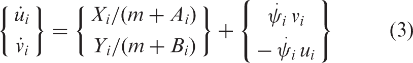Airship dynamics have been studied extensively in the literature which is not a focus of this paper.^3,8,9,21 A standard six degree of freedom model is reduced to three degrees of freedom by removing the vertical translation degree of freedom and the roll and pitch rotations.²² Note that the geometry, mass, and inertia of each airship are assumed to be the same. The kinematic and dynamic equations of motion for the ith airship become

{{x_{i}}^{.} {y_{i}}^{.}} = [c_{ψ_{i}} - s_{ψ_{i}} s_{ψ_{i}} c_{ψ_{i}}] {u_{i} v_{i}}

(1)

{ψ_{i}}^{. .} = \frac{1}{I + R_{i}} N_{i}

(2)

{{\overset{\cdot}{u}}_{i} {\overset{\cdot}{v}}_{i}} = {X_{i} / (m + A_{i}) Y_{i} / (m + B_{i})} + {{ψ_{i}}^{.} v_{i} - {ψ_{i}}^{.} u_{i}}

(3)

where A_i, B_i, and R_i are the apparent masses for the ith airship. These terms are standard for lighter than air vehicles since the mass of the air that is displaced is comparable to the mass (m) and inertia (I) of the airship.³ Standard shorthand notation is used for trigonometric functions:

\cos (α) \equiv c_{α}

and

\sin (α) \equiv s_{α}

. Each airship in this study experiences typical loads associated with standard airship flight, such as aerodynamics (A) and thrust loads (T). However, because each airship operates in close proximity with other airships, contact loads (C) exist when the distance between two airships is less than the diameter of the airship or if the airship encounters a wall. The applied forces (X_i, Y_i) and moments (N_i) expressed in equations (2) and (3) expressed in the body reference frame are given below

{X_{i} Y_{i}} = {X_{A_{i}} + X_{C_{i}} + T_{1_{i}} + T_{2_{i}} Y_{A_{i}} + Y_{C_{i}}}

(4)

N_{i} = N_{A_{i}} + N_{C_{i}} + (T_{2_{i}} - T_{1_{i}}) d

(5)

The airship chosen in this simulation study contains two thrusters a distance d from the center of mass of the airship. Each thruster can be independently controlled and is shown in equation (5) as $T_{1_{i}}$ and $T_{2_{i}}$ .

Aerodynamic model

The body aerodynamic force is calculated using a modified aerodynamic expansion using standard Taylor series aircraft expansion and airship aerodynamics. The airship in this study does not have traditional fins to control pitch and yaw, and the total velocity, V_i, is so small that the dynamic pressure, q_i, can approach zero. This leads to difficulties in modeling yaw damping when the airship is spinning in place.^22,8 The parameter ρ is the atmospheric air density.

{X_{A_{i}} Y_{A_{i}}} = - \frac{1}{2} ρ | V_{i} | {Vol}^{2 / 3} C_{D} {u_{i} v_{i}}

(6)

The total velocity given using the components of velocity (u_i, v_i) in the body frame and computing the magnitude.

V_{i} = \sqrt{u_{i}^{2} + v_{i}^{2}}

(7)

The body aerodynamic moment is also computed using a similarly modified aerodynamic expansion. Note that the dynamic pressure has been modified to allow for yaw damping when no translational velocity is present. This would occur when the airship is simply spinning in place.

N_{A_{i}} = - \frac{1}{2} ρ {Vol}^{5 / 3} | {ψ_{i}}^{.} | (C_{nr} {ψ_{i}}^{.})

(8)

Equations (6) and (8) use the volume (Vol) of the airship as part of its dynamic pressure and can be computed using the relationship below, where b is the diameter of the airship.

Vol = \frac{4}{3} π (b / 2)^{3}

(9)

Finally, equations (6) and (8) contain two aerodynamic coefficients, drag (C_D) and yaw damping (C_nr), which are estimated using a numerical procedure outlined in the Parameter estimation section.

Contact model

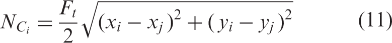
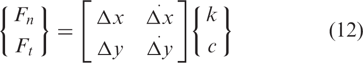
During a collision, contact loads are modeled between bodies which can include either two airships or an airship and a wall. The contact forces are given below

{X_{C_{i}} Y_{C_{i}}} = [c_{ψ_{i}} s_{ψ_{i}} - s_{ψ_{i}} c_{ψ_{i}}] [\hat{e_{p}} \hat{e_{t}}] {F_{n} F_{t}}

(10)

N_{C_{i}} = \frac{F_{t}}{2} \sqrt{(x_{i} - x_{j})^{2} + (y_{i} - y_{j})^{2}}

(11)

where

\hat{e_{p}}

and

\hat{e_{t}}

transform the forces from the contact frame to the inertial frame and the transposed trigonometric matrix transforms the inertial frame forces to the body frame. F_n and F_t represent the contact frame normal force and the tangential force of collision respectively. The yaw moment induced by the contact forces is created by multiplying the tangential force by the distance between the two airships and dividing that value by two. A diagram of these forces and the various frames can be seen in Figure 1. These tangential and normal forces are calculated using spring mass damper equations

{F_{n} F_{t}} = [Δ x {Δ x}^{.} Δ y {Δ y}^{.}] {k c}

(12)

where Δx is the difference between the original radius and the deformed radius from collision and

{Δ x}^{.}

is the difference in velocities of the two airship’s point of contact along a normal axis of contact. Δy will always be zero because the point of collision will be the same for both airships, and

{Δ y}^{.}

is the difference between the velocities of the airships along the tangential axis of contact. The values for k and c are obtained through a numerical integration procedure outline in the Parameter estimation section. Note that it is also possible to have the airship collide with a wall. When this happens the equations are modified such that the position and velocity of the wall remain fixed as opposed to a scenario where two airships collide and can both move.

Figure 1.

Diagram showing the forces of contact and the reference frames.

Formation flight techniques

The main goal is to create formation flight algorithms that reduce computational burden and remove all communication from each airship. Having control laws with no communication between bodies will undoubtedly lead to collisions between airships; however, given the soft structure of an airship, this is not undesirable. Initial ideas centered around simple waypoint tracking where each airship attempts to travel around the same path. There are several methods for waypoint tracking involving a single vehicle.^23–25 However, when multiple vehicles are involved, this task becomes rather complex due to collision avoidance.^11–13 Allowing collisions between each airship reduces the complexity of the controller to the point that each aircraft can operate independently, reducing weight and hardware cost for the vehicle. Thus, a simple waypoint controller is used to control each airship.

For this simulation, proportional–derivative control is used to command the airships to different waypoints ( $x_{W_{i}}, y_{W_{i}}$ ). Using equations (13) to (17), the thrust is altered to guide the airship.

ψ_{W_{i}} = {tan}^{- 1} (\frac{y_{W_{i}} - y_{i}}{x_{W_{i}} - x_{i}})

(13)

Δ ψ_{i} = \tan^{- 1} (\frac{s_{ψ_{i}} c_{ψ_{W_{i}}} - c_{ψ_{i}} s_{ψ_{W_{i}}}}{c_{ψ_{i}} c_{ψ_{W_{i}}} + s_{ψ_{i}} s_{ψ_{W_{i}}}})

(14)

T_{Ni} = k_{pN} (Δ ψ_{i}) + k_{dN} ({ψ_{i}}^{.})

(15)

T_{1_{i}} = (1 - | Δ ψ_{i} | / π) k_{p} (u_{W_{i}} - u_{i}) - \frac{T_{Ni}}{d}

(16)

T_{2_{i}} = (1 - | Δ ψ_{i} | / π) k_{p} (u_{W_{i}} - u_{i}) + \frac{T_{Ni}}{d}

(17)

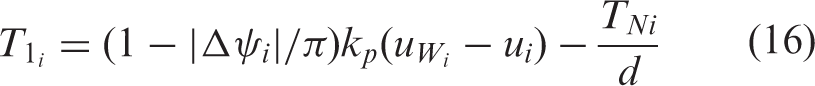
In the equations above, k_p is the velocity proportional gain, k_pN and k_dN are the rotational gains and Δψ_i is the difference between the current yaw angle and the angle needed to face the waypoint. The term $(1 - | Δ ψ_{i} | / π)$ allows the airship to use differential thrust to steer toward its waypoint first and then travel to the waypoint. Since the airship is commanded to move forward only when it is pointing toward the waypoint, it is guaranteed that as long as the airship is pointing toward the waypoint, it will reach the desired waypoint in finite time, assuming no other airships are in its way.

Parameter estimation

In order to model the airship accurately, the airship shown in Figure 2 was purchased to estimate thrust, mass, inertia, aerodynamic coefficients and contact forces.²⁶ The following parameters are all estimated using numerical integration techniques: maximum thrust (T_max), spring constant (k), damping constant (c), drag coefficient (C_D), and yaw damping coefficient (C_nr).

Figure 2.

Model airship −0.965 m diameter.

Mass and inertia

The diameter of the airship is 0.965 m and has a volume of 0.4712 m³, assuming the airship is a perfect sphere. The mass of the airship is found by combining the weight of the structure, gondola and mass of helium, assuming a density of helium equal to 0.18 kg/m³. The mass of the airship is found to 0.1848 kg. The inertia of the airship is found by computing the polar moment of inertia of a sphere and multiplying that value by the mass of the airship. The inertia was found to be 0.0172 kg – m². The distance between the two thrusters is 0.127 m. The air density ρ is set at standard sea level, with a value of 1.225 kg/m³. The derivation for apparent mass can be found in.^27,3 The airship considered in this paper is a special case where the major and minor axes are equal giving an eccentricity of zero. Thus, the rotational apparent mass is zero (R_i = 0). In addition, the translational apparent masses are equal such that A_i = B_i and is given by 8/3(b/2)³. The translational apparent mass was found to be 0.3 kg.

Aerodynamic coefficients

Two experiments were performed to obtain C_D and C_nr. The first experiment involved pushing the airship and measuring the position of the airship over time. The position of the airship was obtained using markers on the ground and wall and using a vision-based technique to extract position. The axial dynamics were then simulated assuming the initial position was zero and the initial velocity was 2.5 m/s. The initial velocity was obtained by differentiating the position using first order finite differencing. A plot of the simulated position and the experimental data can be shown in Figure 3. As seen in this Figure, the simulation matches very well with the experimental data. This is because the drag coefficient was altered until there was agreement between the two models. The drag coefficient obtained was C_D = 0.125. After about 1.2 s into the experiment, significant oscillations in the roll axis were seen. It is believed that this causes the axial position to exhibit some non-linearities.

Figure 3.

Forward position (m) vs. time (s)—forward motion test.

The next experiment was used to obtain the maximum thrust (T_max) and the yaw damping coefficient (C_nr). In this experiment, the airship was initialized with all states equal to zero. The left thruster was then commanded to full power such that the airship began to yaw. The left thrust was held at full power for 7.94 s. The thruster was then turned off and data were obtained for another 10 s.

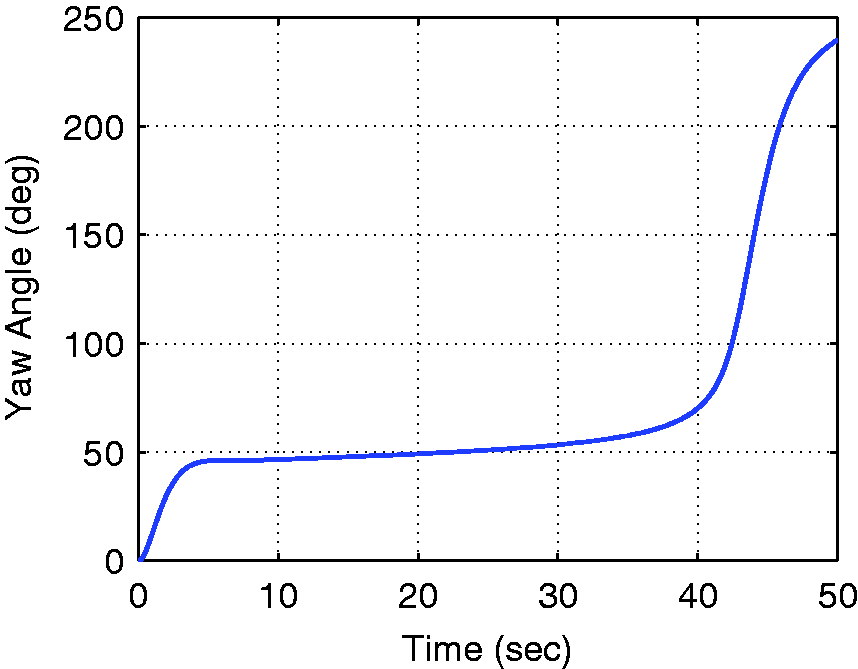
Figure 4 shows that after the parameters are tuned, the simulation and experiment match very well. The yaw angle of the airship was obtained by placing a line on the top of the airship and a vision-based camera to capture the angle as a function of time. Since two parameters were estimated at once, a grid search algorithm was employed to find the optimum solution for T_max and C_nr. The grid search returned a value of T_max = 0.045 N and C_nr = 0.23.

Figure 4.

Yaw angle (deg) vs. time (s)—rotation test.

Spring and damping coefficients

The final experiment performed was used to obtain the spring and damping coefficient of the airships when they collide with each other or a wall. The experiment started with the airship at an initial non-zero forward velocity. After 0.5 s into the experiment, the airship collides with a wall resulting in a negative velocity. Figure 5 shows the position of the airship during this experiment. The position and initial velocity of the airship were obtained in a similar fashion to the forward motion test. Again, since two parameters were estimated at once a grid search was used to find the optimal solution. The grid search returned a value of k = 5.95 N/m and c = 5.90 N – s/m. Note that the simulated data are much smoother, because the airship exhibited non-linear contact dynamics during collision. That is, the amount of compression in the airship was significant. A soft contact model would be better suited to predict collision; however, for initial analysis, a first order model is sufficient.

Figure 5.

Forward position (m) vs. time (s)—collision test.

Controller gains

Once the intrinsic parameters were obtained, the controller gains were also tuned. No grid search was used here since the time response of the airship is up to the control system designer. Thus, the parameters were simply tuned manually until a desirable closed loop time response was found. However, since the controller is designed to rotate the airship toward its target and then command itself to a constant velocity, the rotational gains and translational gains could be tuned independently. First, the rotational gains were tuned and set to k_pN = −0.009 and k_dN = −0.014. Figure 6 shows the airship rotate to a constant yaw angle of 45°. The controller gains were tuned to yield an almost critically damped response while not saturating the thrusters. Using these values for k_pN and k_dN, the yaw angle reaches the commanded yaw angle in about 10 s.

Figure 6.

Yaw angle (deg) vs. time (s)—rotational gain tuning.

With the rotational gains set, the single translational gain could be set to command the airship to a waypoint 10 m in front of it. Figure 7 shows the distance to the waypoint versus time. The simulation stops when the airship reaches its desired waypoint. The value chosen for proportional gain was set to k_p = 0.008, which causes the airship to reach the desired waypoint in about 30 s. In this case, the commanded forward velocity is set to $u_{W_{i}} = 1 m / s$ . The value is set to a low value to ensure that the thrusters do not saturate during complex maneuvers, which would lead to an undesirable response.

Figure 7.

Distance to waypoint (m) vs. time (s)—translational gain tuning.

Finally, to ensure that the controller was properly tuned, the airship was commanded to a waypoint at (10, 10) m. Figure 8 shows the result of the airship traveling to the desired waypoint. This Figure is a top–down view of the airship showing the y-coordinate versus the x-coordinate. Here, the simulation continues even once the airship reaches the waypoint. This Figure also highlights the fact that the controller is not robust. The airship itself does not directly reach the waypoint of (10, 10) m.

Figure 8.

X (m) vs. Y (m).

Figure 9 shows the distance to the waypoint versus time. This Figure shows that the airship only gets within 0.5 m of the waypoint. Figure 10 shows the yaw angle of the airship over time. The airship is initially commanded to rotate to 45° as previously simulated. Once the airship passes the waypoint, the airship must now turn around and it is thus commanded to rotate to 270°. If the simulation was to continue, the airship would begin to circle the waypoint indefinitely.

Figure 9.

Distance to waypoint (m) vs. time (s).

Figure 10.

Yaw angle (deg) vs. time (s).

Multiple airship results

The simulations in this section investigates the performance of five airships in a 5 m wide hall way. The hall way is narrow to encourage collisions to investigate the performance of numerous airships in a small corridor. The first simulation commands the five airships to a single waypoint and the second simulation commands the airships to five unique waypoints. Figure 11 shows each airship travel to one waypoint. The initial x-coordinate of each airship is −10 m and the y-coordinate varies linearly from 0 to 5 m. Each airship is commanded to the point (11, 2.5) m. As can be see in Figure 11, the flight path of all airships is unperturbed until about −5 m in x. At this point, all airships collide with each other. After bouncing around for a few seconds, they all eventually reach the waypoint; however, each airship struggles to maintain its position once it reaches the waypoint. Visualizing collisions using a top–down plot is informative to see how far airships deviate from their intended path, which seems to be about 3 m on the upper end for B3’s path. Figure 12 shows the velocity of all airships as a function of time. This Figure indicates that the path of the two airships is relatively unperturbed until about 20 s. At 20 s, the first collisions occur. These collisions are not that severe given the 10% decrease in velocity. At 60 s into the mission, the airships reach the waypoint or rather they all converge onto the waypoint at the same time and large collisions occur resulting in large deviations in total velocity. In this mission, all airships attempt to travel to the same waypoint, resulting in overcrowding the mission objective. Another type of mission could involve each airship traveling to its own respective waypoint. In this mission, the airships initial conditions are identical but the waypoints start at −1 m and vary linearly until 21 m. Figure 13 shows the result of each airship going to separate waypoints. In this plot, it seems as though the airships have little to no deviations in their path to each waypoint. Airships B3 and B5 seem to have the most deviation. Airship B1 arrives at its waypoint with only slight deviation from its intended path and collides with the wall over and over again resulting in half ellipse shaped paths. Figure 14 shows the velocity of all airships versus time. As expected, B4 and B5 have little to no collisions; however, B1 collides with the top wall around 20 s, whereas B2 does not collide with anything until about 40 s. This is, of course, because the waypoint for B1 is much closer than B2’s waypoint. This velocity plot also indicates that airship B3 has the most difficulty traveling to its waypoint. Still, even with all these collisions, the airships arrive at their waypoints in finite time.

Figure 11.

Simulation of five airships traveling to one waypoint.

Figure 12.

Total velocity (m/s) vs. time (s) for five airships traveling to one waypoint.

Figure 13.

Simulation of five airships traveling to five waypoints.

Figure 14.

Total velocity (m/s) vs. time (s) for five airships traveling to five waypoints.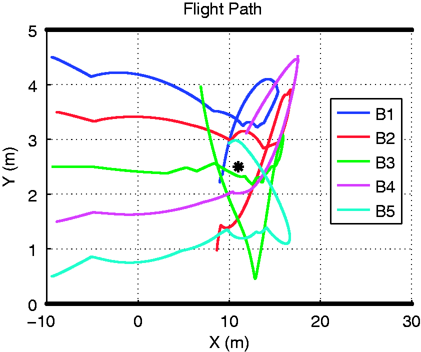

Conclusion

A micro-airship fleet was investigated here where collisions between airships are highly likely given the close proximity of each airship. Given an airships soft structure, airships can collide with other airships and/or its environment without any catastrophic failure provided the severity of the collision is not high enough to puncture the vessel. New types of missions could be performed where collisions are tolerated such as maneuvering indoors. Missions could be created where collisions are encouraged and steering control is completely removed. In this scenario, the only way to deviate from its path is through a collision with a stationary object or another airship. Among other uses, these types of roaming airships could be utilized for indoor missions where time is not a design issue. A three degree of freedom model was developed with simple control laws with no communication between aircraft. This three degree of freedom model was chosen to focus on the feasibility of a micro-airship fleet rather than contributing to the literature on airship dynamics. However, due to the spherical, no fin airship chosen, the standard aerodynamic forces and moments had to be modified to include effects of the airships ability to spin in place. With this dynamic model, parameters were estimated using three tests to obtain the drag coefficient, the max thrust, and yaw damping and a final test to obtain contact coefficients. All of these parameters were placed into a multi-airship simulation to investigate the performance of multiple airships in close proximity. The airships were able to navigate to repeated and discrete waypoints even in a crowded environment. Future work may include surveying a small office building with multiple airships to validate the simulation presented here.

Footnotes

Declaration of conflicting interests

The author(s) declared no potential conflicts of interest with respect to the research, authorship, and/or publication of this article.

Funding

The author(s) received no financial support for the research, authorship, and/or publication of this article.

References

Walter

. Aviation insights: unmanned aerial vehicles. Technology Teacher 2005; 65: 14–19.

Tahk M, Yoo D, Lee C, et al. Optimal resource management algorithm for UAV missions in hostile territories. Proc IMechE, Part G: J Aerosp Eng 2013; 228: 2157–2167.

Zhao Y, Mueller J and Paluszek M. Development of an aerodynamic model and control law design for a high altitude airship. In: AIAA 3rd unmanned unlimited technical conference, workshop and exhibit, Chicago, IL, 20 September–23 September 2004.

Jones

Coleman

Rodgers

. A buoyant life investigating mobile platform (blimp). Adv Space Res 2006; 38: 1198–1208.

Fink

Dohm

Tarbell

et al.

Next-generation robotic planetary reconnaissance missions: a paradigm shift. Planet Space Sci 2005; 53: 1419–1426.

Khoury

. Airship technology, 2nd ed. New York, NY: Cambridge University Press, 2012.

Haley RD. an investigation of the flight dynamics of airships with application to the YEZ-2A. PhD thesis, Cranfield Institute of Technology, UK, 1990.

Ramos JG and Gomes SBV. Airship dynamic modeling for autonomous operations. In: Proceedings of the IEEE International Conference on Robotics and Automation, Leuven, Belgium, 20 May–20 May 1998.

Nahon

Sharf

. Airship dynamics modeling: a literature review. Prog Aero Sci 2011; 47: 217–239.

10.

Takaya

Kawamura

Yamamoto

et al.

Development of the research platform of small autonomous blimp robot. Electronics and Communications in Japan 2008; 91: 1–13.

11.

How J and Richards A. Aircraft trajectory planning with collision avoidance using mixed integer linear programming. In: AIAA conference, Anchorage, AK, 8 May–10 May 2002.

12.

Beard R and McLain T. Trajectory planning for coordinated rendezvous of unmanned air vehicles. In: AIAA Guidance, Navigation, and Control Conference and Exhibit, Denver, CO, 14 August–17 August 2000.

13.

Bellingham JS, Tillerson M, Alighanbari M, et al. Cooperative path planning for multiple UAVs in dynamic and uncertain environments. In: Decision and control, 2002, proceedings of the 41st IEEE conference on, Las Vegas, NV, 10 December–13 December 2002, 3, pp.2816–2822.

14.

Hanson C, Parle J, Allen M, et al. String stability of a linear formation flight control system. In: AIAA guidance, navigation and control conference and exhibit, Monterey, CA, 5 August–8 August 2002.

15.

Hurtado

Wietz

. Investigating time-delay effects for multivehicle formation control. J Aero Comput Inform Comm 2008; 5: 321–336.

16.

Slater G. Dynamics of self-spacing in a stream of in-trail aircraft. In: AIAA guidance, navigation and control conference and exhibit, Monterey, CA, 5 August–8 August 2002.

17.

D’Andrea R and Fowler J. Distributed control of close formation flight. In: IEEE conference on decision and control, Las Vegas, NV, 10 December–13 December 2002.

18.

Murray R and Dunbar W. Model predictive control of coordinated multi-vehicle formations. In: IEEE conference on decision and control, Las Vegas, NV, 10 December–13 December 2002.

19.

Sastry S, Shim D and Kim H. Decentralized nonlinear model predictive control of multiple flying robots. In: IEEE Conference on Decision and Control, Maui, HI, 9 December–12 December 2003.

20.

Lechevin

Rabbath

. Safety and reliability in cooperating unmanned aerial systems, Singapore: World Scientific Publishing Company, 2010.

21.

Choudhry

Ashraf

. Dynamic modeling of the airship with Matlab using geometrical aerodynamic parameters. Aero Sci Tech 2013; 25: 56–64.

22.

Etkins

. Dynamics of atmospheric flight, Dover: NY, 2000.

23.

Yakimeko

. Direct method for rapid prototyping of near-optimal aircraft trajectories. J Guid Contr Dynam 2000; 23: 865–875.

24.

How J, Park S and Deyst J. A new nonlinear guidance logic for trajectory tracking. In: AIAA guidance, navigation, and control conference and exhibit, Providence, RI, 16 August–19 August 2004.

25.

Costello M, Ward M and Montalvo C. Performance characteristics of an autonomous airdrop system in realistic wind environments. In: AIAA GNC/AFM/MST/ASC/ASE conference, Ontario, Canada, 2 August–5 August 2010.

26.

Radio-controlled silver baboom flying saucer UFO (indoor blimp) 27 MHz RC, www.amazon.com/gp/product/B00D61IK9I/ref=s9_simh_gw_p21_d0_i1?pf_rd_m=ATVPDKIKX0DER&pf_rd_s=desktop-1&pf_rd_r=03E3H5E7NJME6WYZKA2N&pf_rd_t=36701&pf_rd_p=2079475242&pf_rd_i=desktop (2015, accessed 2 June 2015).

27.

Tuckerman LB. Inertia factors of ellipsoids for use in airship design. Naca Report. Report no. 210, 1926. Washington, DC: Government Printing Office.